F = xâ1 b Aθ¯r. (4). âFmax ⤠F ⤠Fmax. (5). 0 ⤠Pg ⤠Pg,max. (6). 0 ⤠Pd ⤠Pd0 ..... conversations with Ian Dobson, Daniel Kircshen and Steven Miller about ...
1
Changes in Cascading Failure Risk with Generator Dispatch Method and System Load Level
arXiv:1308.5474v2 [math.OC] 14 Nov 2013
Pooya Rezaei, Student Member, IEEE, Paul D. H. Hines, Member, IEEE
Abstract—Industry reliability rules increasingly require utilities to study and mitigate cascading failure risk in their system. Motivated by this, this paper describes how cascading failure risk, in terms of expected blackout size, varies with power system load level and pre-contingency dispatch. We used Monte Carlo sampling of random branch outages to generate contingencies, and a model of cascading failure to estimate blackout sizes. The risk associated with different blackout sizes was separately estimated in order to separate small, medium, and large blackout risk. Results from N − 1 secure models of the IEEE RTS case and a 2383 bus case indicate that blackout risk does not always increase with load level monotonically, particularly for large blackout risk. The results also show that risk is highly dependent on the method used for generator dispatch. Minimum cost methods of dispatch can result in larger long distance power transfers, which can increase cascading failure risk. Index Terms—Cascading failure risk, Monte Carlo simulation, security-constrained optimal power flow
I. I NTRODUCTION Cascading failure in power systems refers to a sequence of interdependent outages that is initiated by one or more disturbances. Timely operator intervention can often prevent a cascade from resulting in a large blackout; however, large cascades occasionally occur and lead to major blackouts, such as Aug. 2003 [1] or Sept. 2011 [2]. Although large blackouts are low-probability events, they can have catastrophic social and economic impacts. For this reason cascading failure (CF, hereafter) risk assessment is increasingly required by reliability regulations (e.g., from NERC [3]) and is a focus of IEEE Power and Energy Society activities [4]. State-of-the-art CF risk assessment methodologies are documented in [4]. In this paper, we used Monte Carlo simulation to estimate CF risk. Monte Carlo methods are widely used for power system reliability evaluation [5]. However, their application to the problem of estimating CF risk is, on the other hand, much less established in the literature. Standard reliability models typically only calculate the immediate consequence of a sampled outage (such as the direct load shedding that results from a generator outage). Estimating the additional risk posed by the potential for cascading blackouts is more difficult for several reasons. Firstly, the simulation of CF remains a difficult problem, for which little validation data exist, and more research is needed [4]. Secondly, even if a CF can be simulated, the size (in terms of MW of load lost) of a CF can be at any scale, which gives rise to the well documented This work is supported in part by the US Dept. of Energy award #deoe0000447. The authors are with the School of Engineering, University of Vermont, Burlington, VT (e-mail: {pooya.rezaei,paul.hines}@uvm.edu).
power-law in blackout sizes [6], [7]. Thirdly, the size of the search space of all possible n−k contingencies, where n is the number of components that might fail and k is the number that did fail, is enormous and grows exponentially with n and k. Finally, the combinations of outages (and operator errors) that typically trigger CF are usually very low probability and very high impact, further increasing the required computational effort. A few papers have used Monte Carlo sampling for CF risk estimation [8]–[11], and some used sampling techniques to reduce the computational cost of risk estimation. The authors in [8] utilized Monte Carlo simulation and then Importance Sampling to reduce the computational burden. Ref. [9] used correlated sampling in a Monte Carlo simulation to estimate the stress level in the power system. The authors in [10] showed that importance sampling together with variance reduction technique can be used to the increase computational efficiency of CF risk estimation by a factor of 2-4. In [11], the Splitting method was used to produce more substantial speed improvements for a system with both continuous and discrete uncertainty. Non-sampling approaches, such as branching process models [12], [13] provide efficient estimates of risk, but abstract away some details, such as the ability to identify which transmission lines contribute to risk estimates. The authors in [14] and [15] found a phase transition in CF risk when load level changes. In this paper, we are interested to study the impacts of pre-contingency generator dispatch and load level on CF risk. Here, we use the expected value of blackout sizes resulting from random contingencies as our metric of risk. The rest of this paper is organized as follows. Section II discusses the Monte Carlo simulation method. Section III describes the formulation and assumptions for the pre-contingency system. Section IV discusses the simulation and results. Section V explains limitations of the Monte Carlo approach and motivation for future research. Section VI provides our conclusions from this study. II. M ONTE C ARLO S IMULATION In this paper, we estimate CF risk using Monte Carlo (MC) simulation. In each MC iteration, we randomly choose a set of one or more transmission line or transformer (branch) outages randomly, based on the failure rate of each component. Ideally, one would select line outages using a joint probability distribution function for line outages, accounting for correlations among the outage probabilities. Since correlation data are not generally available and correctly modeling correlated line
2
outages requires some care, we assume that line outages are independent here. Accounting for correlations in line outage probabilities remains for future work. Given this assumption, the probability of two (or more) simultaneous outages is the product of each line-failure probability. We use the failure rate of transmission lines (λ, outages/year), and assume that each failure lasts for 1 hour on average. Then, the probability of a line failure at each iteration is computed by pf,i = λi/8760 for all lines, where 8760 is the number of hours in a year. Each random draw in the simulation produces a set of outaged lines with a minimum size of zero. If the size of the outage is 2 or larger (since the system is known to be initially n − 1 secure), this contingency is applied to our cascading failure simulator (CFS), which is explained in [16] in detail. Following the standard MC approach, we use the average (expected) blackout size in MW of load shedding as our measure of risk. The expected value (average) is found by summing over all event sizes and dividing by the number of MC iterations (including events with zero blackout size and zero branch outages). In finding cascading failure risk, it is useful to separately consider risk from events of different sizes. To do so, we add blackout sizes within a certain size range in the numerator and divide by the number of MC iterations, to find the risk associated with blackouts in different size ranges. III. P RE - CONTINGENCY D ISPATCH For the initial results in this paper, we computed the precontingency power flow state for each load level using a Security-Constrained DC Optimal Power Flow (SCDCOPF). As a result, each pre-contingency network is n − 1 secure for any single line outage. Although the DC Optimal Power Flow (DCOPF) is a relatively simple linear programming problem, a full SCDCOPF including all line outages as contingencies can become computationally expensive, especially for larger systems, because of extensive number of contingencies. To reduce the computational effort, we solve a decomposed SCDCOPF based on the method proposed in [17]. The decomposed SCDCOPF is described as follows. Initially, DCOPF is solved to find minimal generation cost dispatch constrained by power flow equations and line flow limits, with the following formulation: min
Pg ,Pd
s.t.
cTg Pg − cTd Pd
(1)
P¯r = Brr θr¯ |G| |D| X X Pg,i = Pd,j
(2)
i=1
(3)
j=1
F = x−1 ¯ b Aθr
(4)
−Fmax ≤ F ≤ Fmax
(5)
0 ≤ Pg ≤ Pg,max
(6)
0 ≤ Pd ≤ Pd0
(7)
where Pg and Pd denote vectors of real power generation and load in the network, and G and D are sets of buses
with generators and loads respectively. cg and cd are vectors of generator marginal costs and the cost of load shedding at each bus, respectively (both in $/M W h). P¯r, Brr and θr¯ are respectively the vector of real power injections, bus susceptance matrix, and the vector of bus voltage angles for all buses except the reference bus. F denotes the line power flow vector. xb is a matrix with each diagonal entry representing the susceptance of each line, and zero non-diagonal entries. A is the node-branch incidence matrix, where the number of rows and columns are equal to the number of branches and buses respectively. Constraints (2) and (3) enforce the DC power flow constraints, and constraint (4) calculates flows from bus voltage angles. Constraints (5), (6) and (7) restrict line flows, real power generation and load to be between their upper and lower bounds. Constraint (7), together with the second term in (1), enables the possibility of load shedding, which ensures that the problem is always feasible. In order to ensure that load shedding does not occur unless absolutely necessary, we set the entries of cd to have large positive values, which are all greater than cg . In this paper, we assume equal values of cd for all loads. In order to make each case n−1 secure, we add contingency constraints. Here, we use the Line Outage Distribution Factors (LODF) matrix to find post-contingency line flows after each line outage [18], which is an m × m matrix, where m represents the number of branches. Assuming line j is tripped in the network, each entry hij of the LODF matrix gives the relative change in flow on line i due to the outage of line j. Therefore, each post-contingency flow constraint has the following form: 0
0
− Fi,max ≤ fi + hij fj ≤ Fi,min
(8)
0
where Fi,max denotes the short term rating of line i. fi and fj denote the pre-contingency power flows on lines i and j respectively. In order to solve a full SCDCOPF, one can add as many as m(m − 1) contingency constraints to the problem. However, explicitly adding these constraints makes problem prohibitively computational expensive, especially for large m. To reduce the computational cost, we implement a decomposed SCOPF, based on [17], in which contingency constraints are incrementally added to the problem until the solution is n − 1 secure. The flowchart of one cycle of this algorithm is shown in Fig. 1. Typically, only 2 or 3 repetitions are needed to find an n − 1 secure solution. IV. S IMULATION AND R ESULTS A. Test Networks We used two test cases to examine how cascading failure risk changes with system load level. First, the 73-bus RTS-96, which has 120 branches and 8550 MW of total load [19]. The pre-contingency DC branch power flows have a mean of 113.8 MW, median of 109 MW, and maximum of 396.1 MW. The second test system is a model of the 2004 winter peak Polish power system that is available with MATPOWER [20]. This test system has 2896 branches (transmission lines and
3
Solve DCOPF k=1
Implement branch “k” outage, and compute power flows
Flow violations?
NO
YES Add constraints for the violated lines to the OPF
k = k+1
Figure 1.
One cycle of the decomposed SCDCOPF (based on [17])
transformers), 2383 buses, and 24.6 GW of total load. The precontingency DC branch power flows have a mean of 34 MW, median of 18.7 MW, and maximum of 882.4 MW. For the Polish case, some of the transmission lines were overloaded in the original system, so we increased line flow limits to be the larger of the current limit and 1.05 times the maximum post-contingency line flows in normal working condition for each line, after increasing all loads by 10%. This ensures that line limits are high enough to serve all loads without load shedding after increasing the base case demand by 10%. Pre-contingency test cases were prepared for both systems using the SCDCOPF method from Sec. III, for a range of load levels from 50% to 119%. 119% was the highest load factor for which SCDCOPF could find a solution without load shedding in the RTS-96 case. For the Polish system, load could increase up to 110% without load shedding. However, we extended our study up to 115% for comparison, which caused less than 1% load shedding in the SCDCOPF solution for cases above 110% load level. Finally, Monte Carlo simulation was performed for both test networks, for each load level. B. RTS-96 Results Fig. 2 shows cascading failure risk, in terms of the expected value of blackout sizes, for two pre-contingency dispatch conditions for the RTS case. Panel (a) shows the results after using SCDCOPF at each load level. Each point on the graph shows the rolling average of risk across 3 consecutive integer percentage load levels (i.e., the datum at 90% load is the average risk for 89%, 90%, and 91%). As previously mentioned, the risk associated with different blackout sizes are separately presented. It is interesting to note that small blackout risk is relatively uniform across all load levels, with a peak at around 80% load level, whereas large blackout risk is largest at about 70% load level, and decreases significantly
as the load level increases. Fig. 2 panel (b) shows CF risk with a proportional dispatch method. To obtain these dispatch cases, we took the 119% load level case from SCDCOPF, and uniformly decreased the loads and generators to each smaller load level. Interestingly, this dispatch approach reduces risk substantially. Furthermore, what risk remains is purely due to small blackouts (BO sizes < 5%). The pre-contingency dispatch in this case is obviously more expensive that that from the SCDCOPF, which suggests that there is an important tradeoff between generation dispatch costs and CF risk. In order to understand the reason behind this difference, we looked at the power flows on five critical lines that connect the three areas in the RTS-96 system. An outage on these lines can cause the system to separate into islands. If this occurs and there is not enough generation and time to allow generators to ramp up or down after the network separates into islands, a large amount of load shedding may occur. The line flow results in Table I show that the flows are generally much higher at the 50% and 75% load levels of the SCDCOPF dispatch than at the 119% level. On the other hand, for the proportional dispatch case, the power flows change more uniformly as load changes. These results suggest that the SCDCOPF algorithm is using more long-distance transmission at moderate load levels, whereas at higher load levels important transmission corridors are not loaded as close to their capacity. C. Polish System Results The same MC sampling approach was implemented on the Polish grid, as explained in Section IV-A. Here, we only use SCDCOPF for the pre-contingency dispatch. Fig. 3 shows CF risk for all blackout sizes (top), and for only large blackouts (bottom). This figure shows that there is a high risk associated with small blackouts (BO sizes < 10%), which increases uniformly with load level. This result is largely due to the fact that the Polish test case has numerous loads on radial lines, the failure of which can cause load shedding in the downstream system. Although larger blackouts are less likely, their outcomes can be catastrophic. Therefore, in this paper, we are mostly concerned with large blackouts from cascading failure. Fig. 3 (bottom) shows CF risk associated with blackout sizes greater than 10% separately for each 10% interval. We see that the pattern of these blackouts no longer changes uniformly with load level. It is also worth noting that CF risk decreases for load percentages higher than 110% (the same cases for which some load shedding, less than 1%, occurs during the pre-contingency dispatch). V. L IMITATIONS OF THE M ONTE C ARLO A PPROACH AND F UTURE W ORK The expected value of a random variable (blackout size in our study) can be found if we know the probability distribution function of that random variable. Given our assumption that the results of a given contingency are deterministic, if we can find all branch combinations that cause a blackout, then CF risk is: X R(x) = Pr(c)S(c, x) (9) c∈C
4
Risk (Expected BO size, kW)
0.45
BO