MARINE ECOLOGY PROGRESS SERIES Mar Ecol Prog Ser
Vol. 213: 229–240, 2001
Published April 4
Changes in copepod distributions associated with increased turbulence from wind stress L. S. Incze1,*, D. Hebert 2, N. Wolff1, N. Oakey 3, D. Dye1 2
1 Bigelow Laboratory for Ocean Sciences, West Boothbay Harbor, Maine 04575, USA Graduate School of Oceanography, University of Rhode Island, Kingston, Rhode Island 02882, USA 3 Bedford Institute of Oceanography, Dartmouth, Nova Scotia B2Y 4A2, Canada
ABSTRACT: Vertical profiles of turbulent kinetic energy dissipation rate (ε), current velocity, temperature, salinity, chlorophyll fluorescence, and copepods were sampled for 4 d at an anchor station on the southern flank of Georges Bank when the water column was stratified in early June 1995. Copepodite stages of Temora spp., Oithona spp., Pseudocalanus spp., and Calanus finmarchicus, and all of their naupliar stages except for Temora spp., were found deeper in the water column when turbulent dissipation rates in the surface mixed layer increased in response to increasing wind stress. Taxa that initially occurred at the bottom of the surface mixed layer at 10 to 15 m depth (ε ≤ 10– 8 W kg–1) before the wind event were located in the pycnocline at 20 to 25 m depth when dissipation rates at 10 m increased up to 10– 6 W kg–1. Dissipation rates in the pycnocline were similar to those experienced at shallower depths before the wind event. After passage of the wind event and with relaxation of dissipation rates in the surface layer, all stages returned to prior depths above the pycnocline. Temora spp. nauplii did not change depth during this period. Our results indicate that turbulence from a moderate wind event can influence the vertical distribution of copepods in the surface mixed layer. Changes in the vertical distribution of copepods can impact trophic interactions, and movements related to turbulence would affect the application of turbulence theory to encounter and feeding rates. KEY WORDS: Turbulence · Zooplankton · Vertical distribution · Vertical migration · Chlorophyll maximum · Stratification · Mixing Resale or republication not permitted without written consent of the publisher
INTRODUCTION Pelagic environments are characterized by vertical changes in light, temperature, turbulence, transport, food and predators. These conditions vary non-uniformly in space and time. As a result, zooplankton face a highly variable environment in which to feed, mate, avoid predators and recruit to satisfactory habitats. The vertical distribution patterns and movements of zooplankton reflect evolved strategies for dealing with these conditions. In turn, the vertical distributions affect other processes, such as feeding by planktivorous fishes. Despite the importance of vertical position to vital rate functions (feeding, respiration, reproduc*E-mail:
[email protected] © Inter-Research 2001
tion) and trophic interactions, only a few of the possible environmental stimuli and corresponding zooplankton responses are known well enough to be predictive. For example, in the past, different studies provided conflicting evidence about the prevailing depth distribution patterns of species and diel patterns of vertical migrations (DVM: Hays et al. 1997). Recent findings have shown substantial plasticity in DVM patterns when certain predators are present (Neill 1990, 1992, Ohman 1990, Bollens & Stearns 1992, Frost & Bollens 1992). This accounts for some of the prior conflicting data and suggests that the risk of predation weighs heavily among the factors influencing this behavior. Turbulent mixing also affects zooplankton behavior (Costello et al. 1990, Saiz & Alcaraz 1992, Saiz 1994) and has been associated with changes in zooplankton
230
Mar Ecol Prog Ser 213: 229–240, 2001
vertical distributions (Buckley & Lough 1987, Mackas et al. 1993, Haury et al. 1990,1992, Incze et al. 1990, Checkley et al. 1992, Lagadeuc et al. 1997). Moreover, small-scale turbulence may directly affect feeding rates of zooplankton (Yamazaki et al. 1991, Kiørboe & Saiz 1995, Saiz & Kiørboe 1995, Osborn 1996) and larval fish (Dower et al. 1997, MacKenzie & Kiørboe 1995, 2000) through changes in shear velocities and modifications of feeding and searching behavior (Saiz 1994, Mackenzie & Kiørboe 1995). While the intensity of turbulence in the upper ocean is strongly correlated with the wind stress (Oakey & Elliott 1982, Mackenzie & Leggett 1991), the vertical structure of small-scale turbulence may be quite complicated (Denman & Gargett 1988, Gargett 1989). This places limits on the usefulness of proxy variables for estimating turbulence at discrete depths and inferring behavioral and other rate functions for the resident plankton (Mullin et al. 1985, Yamazaki & Osborn 1988, Simpson et al. 1996, Gargett 1997). Since turbulence is ubiquitous and highly variable, a better understanding of zooplankton responses to changing turbulence, as well as any preferences for certain ranges, is needed in order to predict and interpret distributions and their biological consequences. At the same time, better information is needed concerning the structure of turbulence within the surface mixed layer and the pycnocline, where many of the biological interactions take place. In this paper we examine the relationship between measured, in situ turbulence and the vertical position of several abundant copepod taxa on the stratified southern flank of Georges Bank, off the northeastern coast of the USA. Georges Bank, historically noted for its high fisheries production (Brown 1987), is approximately 300 km long × 175 km wide. The crest of the bank (< 50 m deep) remains mixed throughout the year by the combined energy of winds and strong tidal currents (Horne et al. 1996), while at depths > 60 m the water column becomes stratified during warm months of the year. Stratification begins in May and lasts until fall, when it is eroded by seasonal surface cooling and increased wind mixing (Flagg 1987). Residual circulation is clockwise around the bank and is well developed during the stratified period (Butman et al. 1987, Limeburner & Beardsley 1996). The physics and biology of the bank are being investigated through the current US and Canadian GLOBEC programs (Wiebe et al. 2001), of which this study is a part.
MATERIALS AND METHODS Data were collected on the southern flank of Georges Bank from 11 to 15 June 1995. The vessel was an-
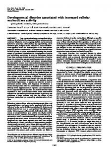
chored at 40.86° N, 67.54° W throughout the sampling period in a nominal depth of 75 m of water (Fig. 1). Microstructure measurements of temperature, salinity and velocity were made with a tethered free-fall profiler (EPSONDE: Oakey 1988) that was deployed from the stern of the vessel and descended at 0.5 to 1 m s–1 until it hit the bottom. The sensor package was recessed 5 cm behind a circular, 30 cm-diameter, stainless steel lander. The tether was a kevlar multiconductor payed out loosely ahead of the falling profiler and used for data transmission and instrument recovery. Velocity fluctuations were measured by 2 shear probes sampling at 256 Hz. From 10 to 20 profiles were collected in rapid succession over a 0.5 to 1.7 h time period and were grouped into ‘sample ensembles’. Ensembles were initiated, on average, every 2.4 h except for a period of adverse winds and current directions. Turbulent kinetic energy dissipation rates (ε, in units of W kg–1) were derived from the velocity fluctuation profiles (Oakey & Elliott 1982). The data were analyzed in 2 s segments blocked so that the last segment ended on the last data point where the instrument was still falling. Power spectra for the 2 shear profiles were computed, frequency-response corrections for the sensors and electronic transfer were applied, and variance due to spikes and noise was removed (Oakey 1982). All of the profiles in an ensemble were averaged together in 2 dbar depth bins using the maximum likelihood estimator for a lognormal distribution (Baker & Gibson 1987). Data from the upper 8 m were not used because they were contaminated by turbulence created by the current flowing past the anchored research vessel.
Fig. 1. Portion of the southern flank of Georges Bank showing location (+) where RV ‘Seward Johnson’ anchored for microstructure and zooplankton profiling on 11 to 15 June 1995. Open square measures 20 × 20 km and encompasses the water area advected past the anchor station during the course of measurements (cf. Fig. 6); solid circle shows location of NOAA Buoy 44011
Incze et al.: Copepod distributions and wind-induced turbulence
Zooplankton in the upper 50 m of the water column were collected at discrete depths using a pumping system connected to a CTD. Collections were made during daylight hours between microstructure profiling sessions. Our strategy was to sample at 5 m intervals or less until we were at 40 m, adding samples around major fluorescence features and density (σt ) gradients. Each zooplankton profile thus was constructed from individual collections made at 10 to 12 depths. The sampling system consisted of the following elements: (1) a PVC hose, 4 cm inside diameter and 60 m long, was attached to the CTD/rosette frame so that the opening was at the same depth as the CTD sensors; (2) a centrifugal pump submerged near the surface delivered 1 m3 min–1 from the sampling depth to a manifold on deck; and (3) a smaller hose, 1.9 cm inside diameter, was connected to the manifold and removed 30 l min–1 from the main flow. We sampled the small flow for 1 min, filtering the water through individual 40 µm-mesh samplers and preserving the retained zooplankton in 5% buffered formalin. When pumping, the CTD was stopped at desired depths long enough to clear the system entirely before we commenced sampling. The CTD record showed that the intake depth never varied by more than ±1 m from the intended depth, and usually the range was ± 0.5 m or less. In the laboratory, zooplankton samples were analyzed in 2 stages. First, we counted all copepodites and nauplii from each sample without further taxonomic identification. Abundance data (number l–1) were used to examine changes in vertical distribution and total abundance (upper 50 m) over the 4 d of sampling. Then, for a subset of the profiles, we identified the species and developmental stages of the most abundant copepods to the lowest taxonomic level possible. The subset consisted of 3 d of sampling centered around a wind event where changes in the vertical distribution of copepods occurred. The enumerated taxa were Temora spp., Oithona spp., Pseudocalanus spp., and Calanus finmarchicus. To look at changes in the vertical distributions of each taxon over time, we standardized each profile so that the highest concentration for a given taxon in that profile had a value of ‘1’. All other concentrations for that taxon in that profile were scaled to the highest concentration to give a relative concentration (0.3, 0.4, etc.) at every other depth sampled in the profile. Vertical distributions were contoured for the set of profiles (that is, over time) by kriging the data. When kriging, we adjusted horizontal tension (anisotropy, up to a factor of 2) to make smooth connections between profiles. This was necessary because data density was much greater in the vertical dimension (5 m or less) than in the horizontal (sample spacing of ~8 h during the day and ~14 h between days).
231
We used the ship’s 150 kHz broad-band acoustic doppler current profiler (ADCP) to analyze water movements past the anchor site. Data were binned into 2 m depth intervals, averaged into 2 min ensembles, and corrected with bottom tracking data to provide estimates of absolute water velocity and direction. Horizontal velocities had a standard deviation of 0.8 cm s–1. Wind speed came from the ship’s anemometer and from NOAA Buoy 44011, located 84 km to the east (Fig. 1). Wind speeds were corrected to a standard height of 10 m (Large & Pond 1981).
RESULTS We completed 10 CTD/pump profiles over 4 d at the stratified site. With only a few exceptions, copepodites and copepod nauplii were most abundant in the upper 20 m. Nauplii showed a tendency for shallower distributions than the copepodites. A subsurface chlorophyll maximum layer was present for the first half of the series near the base of the pycnocline (Fig. 2). Except for Profile 106, most of the copepodites and the nauplii were above this feature. The depth of the pycnocline and the shape of the density profiles changed throughout the series, although surface and bottom σt values changed only slightly. There was no consistent relationship between the pycnocline and the depths of the copepod stages. In Profiles 106 and 115, copepodites assumed a deeper distribution than at other times. The nauplii at these 2 stations exhibited a variable vertical pattern, not as focussed as that for the copepodites but with some deepening compared with other nauplii profiles. Naupliar profiles at both these stations showed reduced abundances at 20 m, with higher concentrations both above and below. We examined the taxonomic composition of the most abundant copepods in the upper 25 m in Profiles 81 to 141. These data covered a 3 d period which included 1 d before and after the deepening of copepod stages in Profiles 106 and 115. The number of individuals of each species in samples collected below 25 m was always low, and for that reason we did not include them in this analysis. A broad range of copepodite and naupliar stages was found (Table 1). Copepodite stages (Fig. 3A) of Temora spp. and Oithona spp. showed shallow distributions of 10 to 15 m on the first day, a deepening to 25 m on the second day, and a return to shallower depths on the third. Most Pseudocalanus spp. began the series at about 15 m and underwent some deepening and then shoaling on the second and third days, respectively. Another change in this genus occurred in the upper 15 m, where the proportion of copepodites decreased markedly during the second day. Most of the Calanus fin-
232
Mar Ecol Prog Ser 213: 229–240, 2001
Index
0
FI
0
A. Copepodites
4 4
σt 24.8
0
25.8
*
*
*
Depth (m)
20 40 60
81
89
106
92
80
*
137
*
B. Nauplii
141
161
163
*
*
0
Depth (m)
129
115
*
*
*
20 40 60
81
89
Year Day 162.53 (GMT)
106
92
80
* 162.76
129
115
137
*
162.95
163.57
141
161
*
163.93
164.57
164.76
164.94
163 *
165.83
165.95
Fig. 2. (A) Vertical profiles of total copepodite stage abundance (•), fluorescence, FL (continuous line) and sigma-t density (broken line) on 11 to 14 June; profile numbers are underlined; all profiles were taken during daylight between 10:00 and 18:45 h; asterisks mark the last sample of each day, all taken between 18:00 and 18:45 h; copepodite abundances are index values (0 to 1.0) which are scaled to the highest abundance in each profile to emphasize the relative vertical patterns; open circles surround index values ≥ 0.5 (i.e., where the concentration, no. l–1, was ≥ 50% of the maximum concentration found in that profile); changes in abundance over time are shown in Fig. 8. (B) Vertical profiles of total naupliar stage abundance; further details as in (A). Time at the beginning of each profile is given at the bottom as year-day (GMT) for reference to other figures
Table 1. Mean stage composition (proportions) of copepodite (CI to CVI) and naupliar (NI to NVI) stages of dominant copepod taxa in Zooplankton Profiles 81 to 141 Taxon Temora spp. Oithona spp. Pseudocalanus spp. Calanus finmarchicus Taxon Temora/Centropages spp.a Oithona spp. Pseudocalanus/Metridia spp.a Calanus finmarchicus a
CI
CII
CIII
CIV
CV
CVI
0.31 0.02 0.25 0.39
0.28 0.05 0.11 0.14
0.23 0.07 0.08 0.23
0.14 0.13 0.11 0.23
0.03 0.29 0.14 0.00
0.02 0.44 0.32 0.00
NI
NII
NIII
NIV
NV
NVI
0.07 0.23 0.26 0.23
0.26 0.15 0.17 0.14
0.24 0.26 0.26 0.31
0.20 0.18 0.26 0.16
0.14 0.10 0.04 0.15
0.09 0.08 0.01 0.02
Nauplii of these taxa are difficult to distinguish. However, few Metridia or Centropages spp. copepodites were found in the samples, so we assume most nauplii belonged to the genera Pseudocalanus and Temora, respectively
marchicus copepodites were deep (below 20 m) to begin with, although some were found near the surface. None were found above 20 m on the second day. Among the nauplii (Fig. 3B), the patterns varied between species. Temora spp. showed no discernible change over time. (Temora spp. were grouped with Centropages spp. because the early naupliar stages could not be distinguished between the 2 genera; however, adult Centropages were rare in these samples, and we therefore believe that most nauplii belonged to the abundant Temora.) Oithona spp. showed a deepening which appeared late in the second day, in Profile 115. Pseudocalanus spp. and Calanus finmarchicus had lower concentrations above 20 m in Profile 115 than they had at other times. (Pseudocalanus spp. are
233
Incze et al.: Copepod distributions and wind-induced turbulence
–5
A. Copepodites
Temora
–5
–10
–10
–15
–15
–20
–20
–25
Temora/Centropages
B. Nauplii
–25 Oithona
Oithona
–5
–5
–10
–10
–15
–15
–20
–20 Depth (m)
Depth (m)
1 .0
–25 –5
Pseudocalanus
–5
–10
–10
–15
–15
–20
–20
–25 –5
0 .8
–25 0 .6
Pseudocalanus
0 .4 0 .2
–25 Calanus
–5
–10
–10
–15
–15
–20
–20
–25
0 .0 Calanus
–25 163
81
92
163.5 164 Year Day (GMT)
106
115
164.5
129
163
141
81
92
163.5 164 Year Day (GMT)
106
Profile
115
164.5
129
141
Profile
Fig. 3. Vertical distributions of (A) copepodites and (B) nauplii of abundant copepod taxa in the surface mixed layer during 3 d (11 to 13 June), with a wind event on the second day. Shaded contours show index values (0.2 gradations) during daylight hours, as in Fig. 2
grouped with Metridia spp. because the naupliar stages are difficult to distinguish, but adult female Metridia spp. were rare on the southern flank.) Table 2 summarizes the abundances of taxa used in Fig. 3; we simplified the table by using the names Temora and Pseudocalanus spp. without the other possible genera. The ship’s meteorological data acquisition system was not working from Year Day 164.5 to 165.5, a period of light wind following the principal wind event. We used wind data from NOAA Buoy 44011 to fill in during this period. Wind speed data from the ship were highly correlated with the buoy record when both systems were operating during this study (n = 84 hourly comparisons, r2 = 0.75, p