Changes in Streamflow and Water Quality in ... - Semantic Scholar

Changes in Streamflow and Water Quality in Selected Nontidal Sites in the Chesapeake Bay Basin, 1985-2003 by Michael J. Langland, Scott W. Phillips, Jeff P. Raffensperger, and Douglas L. Moyer

In cooperation with the U.S. Environmental Protection Agency, Chesapeake Bay Program; the Maryland Department of Natural Resources; and the Virginia Department of Environmental Quality

Scientific Investigations Report 2004-5259

U.S. Department of the Interior U.S. Geological Survey

U.S. Department of the Interior Gale A. Norton, Secretary U.S. Geological Survey Charles G. Groat, Director

U.S. Geological Survey, Reston, Virginia: 2004 For sale by U.S. Geological Survey, Information Services Box 25286, Denver Federal Center Denver, CO 80225

For more information about the USGS and its products: Telephone: 1-888-ASK-USGS World Wide Web: http://www.usgs.gov/ Any use of trade, product, or firm names in this publication is for descriptive purposes only and does not imply endorsement by the U.S. Government. Although this report is in the public domain, permission must be secured from the individual copyright owners to reproduce any copyrighted materials contained within this report.

Suggested citation: Langland, M.J., Phillips, S.W., Raffensperger, J.P., and Moyer, D.L., 2004, Changes in streamflow and water quality in selected nontidal sites in the Chesapeake Bay Basin, 1985-2003: U.S. Geological Survey Scientific Investigations Report 2004-5259, 50 p.

iii

Contents Abstract. . . . . . . . . . . . . . . . . . . . . . . . . . . . . . . . . . . . . . . . . . . . . . . . . . . . . . . . . . . . . . . . . . . . . . . . . . . . . . . . . . . . . . . . . . . . . . . . . . . . . 1 Introduction . . . . . . . . . . . . . . . . . . . . . . . . . . . . . . . . . . . . . . . . . . . . . . . . . . . . . . . . . . . . . . . . . . . . . . . . . . . . . . . . . . . . . . . . . . . . . . . . 1 Purpose and Scope. . . . . . . . . . . . . . . . . . . . . . . . . . . . . . . . . . . . . . . . . . . . . . . . . . . . . . . . . . . . . . . . . . . . . . . . . . . . . . . . . . . 2 Methods and Approach. . . . . . . . . . . . . . . . . . . . . . . . . . . . . . . . . . . . . . . . . . . . . . . . . . . . . . . . . . . . . . . . . . . . . . . . . . . . . . . 2 Data-Set Construction . . . . . . . . . . . . . . . . . . . . . . . . . . . . . . . . . . . . . . . . . . . . . . . . . . . . . . . . . . . . . . . . . . . . . . . . . . . . . . . . 2 Description and Evaluation of Methods and Techniques. . . . . . . . . . . . . . . . . . . . . . . . . . . . . . . . . . . . . . . . . . . . . . . 5 Streamflow. . . . . . . . . . . . . . . . . . . . . . . . . . . . . . . . . . . . . . . . . . . . . . . . . . . . . . . . . . . . . . . . . . . . . . . . . . . . . . . . . . . . . . 5 Load Computations. . . . . . . . . . . . . . . . . . . . . . . . . . . . . . . . . . . . . . . . . . . . . . . . . . . . . . . . . . . . . . . . . . . . . . . . . . . . . . 6 Concentrations. . . . . . . . . . . . . . . . . . . . . . . . . . . . . . . . . . . . . . . . . . . . . . . . . . . . . . . . . . . . . . . . . . . . . . . . . . . . . . . . . . 7 Observed . . . . . . . . . . . . . . . . . . . . . . . . . . . . . . . . . . . . . . . . . . . . . . . . . . . . . . . . . . . . . . . . . . . . . . . . . . . . . . . . . . 7 Flow-Weighted . . . . . . . . . . . . . . . . . . . . . . . . . . . . . . . . . . . . . . . . . . . . . . . . . . . . . . . . . . . . . . . . . . . . . . . . . . . . 7 Flow-Adjusted . . . . . . . . . . . . . . . . . . . . . . . . . . . . . . . . . . . . . . . . . . . . . . . . . . . . . . . . . . . . . . . . . . . . . . . . . . . . . 8 Summary of Changes in Methods . . . . . . . . . . . . . . . . . . . . . . . . . . . . . . . . . . . . . . . . . . . . . . . . . . . . . . . . . . . . . . . 8 Changes in Streamflow. . . . . . . . . . . . . . . . . . . . . . . . . . . . . . . . . . . . . . . . . . . . . . . . . . . . . . . . . . . . . . . . . . . . . . . . . . . . . . . . . . . . . . 9 Annual Mean Flow . . . . . . . . . . . . . . . . . . . . . . . . . . . . . . . . . . . . . . . . . . . . . . . . . . . . . . . . . . . . . . . . . . . . . . . . . . . . . . . . . . . 9 Quarterly Mean Flow. . . . . . . . . . . . . . . . . . . . . . . . . . . . . . . . . . . . . . . . . . . . . . . . . . . . . . . . . . . . . . . . . . . . . . . . . . . . . . . . . 11 Changes in Water Quality . . . . . . . . . . . . . . . . . . . . . . . . . . . . . . . . . . . . . . . . . . . . . . . . . . . . . . . . . . . . . . . . . . . . . . . . . . . . . . . . . . 11 Observed Concentrations . . . . . . . . . . . . . . . . . . . . . . . . . . . . . . . . . . . . . . . . . . . . . . . . . . . . . . . . . . . . . . . . . . . . . . . . . . . . 11 Flow-Weighted Concentration . . . . . . . . . . . . . . . . . . . . . . . . . . . . . . . . . . . . . . . . . . . . . . . . . . . . . . . . . . . . . . . . . . . . . . . 19 Flow-Adjusted Concentration . . . . . . . . . . . . . . . . . . . . . . . . . . . . . . . . . . . . . . . . . . . . . . . . . . . . . . . . . . . . . . . . . . . . . . . . 19 Loads . . . . . . . . . . . . . . . . . . . . . . . . . . . . . . . . . . . . . . . . . . . . . . . . . . . . . . . . . . . . . . . . . . . . . . . . . . . . . . . . . . . . . . . . . . . . . . . 23 Summary and Conclusions . . . . . . . . . . . . . . . . . . . . . . . . . . . . . . . . . . . . . . . . . . . . . . . . . . . . . . . . . . . . . . . . . . . . . . . . . . . . . . . . . 27 References Cited. . . . . . . . . . . . . . . . . . . . . . . . . . . . . . . . . . . . . . . . . . . . . . . . . . . . . . . . . . . . . . . . . . . . . . . . . . . . . . . . . . . . . . . . . . . 28 Appendix 1. Quarterly-mean streamflow for the Choptank, Patuxent , Appomattox, Rappahannock, Pamunkey, and Mattaponi Rivers, 1985-2003. . . . . . . . . . . . . . . . . . . . . . . . . . . . . . . . . . . . . . . . . . . . . . . . . . . . . . . 29 Appendix 2. Statistical summaries for water-quality concentration data for total nitrogen (A), total phosphorus (B), and sediment (C) for the Choptank, Patuxent, Rappahannock, Mattaponi, Pamunkey, and Appomattox Rivers. . . . . . . . . . . . . . . . . . . . . . . . . . . . . . . . . . . . . . . . . . . . . . . . . . . . . . . . . . . . . . . . 33 Appendix 3. Trends in flow-adjusted concentration data for 9 River Input Monitoring Program sites and 24 Multi-Agency Nontidal Program Sites in the Chesapeake Bay Watershed, 1985-2003 . . . . . . 41

Figures 1. Map showing location and site number for the 33 sites used in this study, Chesapeake Bay watershed . . . . . . . . . . . . . . . . . . . . . . . . . . . . . . . . . . . . . . . . . . . . . . . . . . . . . . . . . . . . . . . . . . . . . . . . . . . . . . . . . . . . . . . . .3 2. Boxplot showing the percent change in magnitude using the revised equation (linear and quadratic coefficients) to estimate trend as compared to the old method (linear coefficient) . . . . . . . . . . . . . . . . . . . . . . . . . . . . . . . . . . . . . . . . . . . . . . . . . . . . . . . . . . . . . . . . . . . . . . . . . . . . . . . . . .9 3. Graph showing variation in annual mean flow entering the Chesapeake Bay, 1935-2003, using computations as described in Bue (1968) . . . . . . . . . . . . . . . . . . . . . . . . . . . . . . . . . . . . . . . . . . . . . . . . . . . 10 4. Graphs showing quarterly mean streamflow for the Susquehanna (1985-2003), Potomac (1985-2003), and James (1989-2003) Rivers . . . . . . . . . . . . . . . . . . . . . . . . . . . . . . . . . . . . . . . . . . . . . . . . . . . . . . . . 12

iv

Figures—Continued 5. Boxplots showing range in observed concentrations for the nine River Input Monitoring sites, Chesapeake Bay watershed, 1985-2003. . . . . . . . . . . . . . . . . . . . . . . . . . . . . . . . . . . . . . . . . . . . . . . . . . . . . . . . . . . 15 6. Boxplots showing annual distribution of observed total nitrogen, total phosphorus, and sediment concentrations collected at the River Input Monitoring sites for the Susquehanna (A), Potomac (B), and James Rivers (C) in the Chesapeake Bay watershed, 1984-2003. . . . . . . . . . . . . . . . . . . . . . . . . . . . . . . . . . . . . . . . . . . . . . . . . . . . . . . . . . . . . . . . . . . . . . . . . . . . . . . . . . . . . . . . . 16 7. Graphs showing flow-weighted concentrations for the Susquehanna, Potomac, and James Rivers entering the Chesapeake Bay for 1988-2003. . . . . . . . . . . . . . . . . . . . . . . . . . . . . . . . . . . . 20 8-10. Maps showing: 8. Trends in flow-adjusted concentrations for total nitrogen, Chesapeake Bay watershed, 1985-2003 . . . . . . . . . . . . . . . . . . . . . . . . . . . . . . . . . . . . . . . . . . . . . . . . . . . . . . . . . . . . . . . . . . . . . . . . . . . . . . . . . . . . . 21 9. Trends in flow-adjusted concentrations for total phosphorus, Chesapeake Bay watershed, 1985-2003 . . . . . . . . . . . . . . . . . . . . . . . . . . . . . . . . . . . . . . . . . . . . . . . . . . . . . . . . . . . . . . . . . . . . . . . . . . . . . . . . . . . . . 22 10. Trends in flow-adjusted concentrations for sediment, Chesapeake Bay watershed, 1985-2003 . . . . . . . . . . . . . . . . . . . . . . . . . . . . . . . . . . . . . . . . . . . . . . . . . . . . . . . . . . . . . . . . . . . . . . . . . . . . . . . . . . . . . 24 11-12. Graphs showing: 11. Significance and range in magnitude in trend for flow-adjusted concentrations from the ESTIMATOR model for the nine River Input Monitoring sites, Chesapeake Bay watershed, 1985-2003 . . . . . . . . . . . . . . . . . . . . . . . . . . . . . . . . . . . . . . . . . . . . . . . . . . . . . . . . . . . . . . . . . . . . . . . . . . . . . . . . . . . . . 25 12. Combined annual flow and total nitrogen, total phosphorus, and sediment load for the nine River Input Monitoring sites flowing into the Chesapeake Bay for 1990-2003. . . . . . . . . . . . . . . 26

Tables 1. Streamflow and water-quality station numbers for the 9 River Input Monitoring Program and 24 Multi-Agency Program sites. . . . . . . . . . . . . . . . . . . . . . . . . . . . . . . . . . . . . . . . . . . . . . . . . . . . . . . . . . . . . . . . . . . . . . 4 2. Nitrogen, phosphorus, and sediment species tested for trend . . . . . . . . . . . . . . . . . . . . . . . . . . . . . . . . . . . . . . . . 5 3. Summary of trend tests, results of evaluations, and suggested approaches used in this report. . . . . . . 10 4. Minimum, mean, median, and maximum concentrations of total nitrogen, total phosphorus, and suspended sediment at the 9 River Input Monitoring sites and 25 Multi-Agency Nontidal Program sites in the Chesapeake Bay watershed . . . . . . . . . . . . . . . . . . . . . . . . . . . . . . . . . . . . . . . . . . . . . . . . . . 13 5. Significant trend direction for the above-normal streamflow in 2003 (1985-2003 trends) and below-normal streamflow in 2002 (1985-2002 trends) calendar years. . . . . . . . . . . . . . . . . . . . . . . . . . . . . . . . 27

v

Conversion Factors and Datum Multiply

square mile (mi2)

cubic foot per second (ft3/s)

pound, avoirdupois (lb) ton per year (ton/yr)

By Area 2.590 Flow rate 0.02832 Mass 0.4536 0.9072

To obtain

square kilometer (km2)

cubic meter per second (m3/s)

kilogram (kg) metric ton per year (ton/yr)

Vertical coordinate information is referenced to the North American Vertical Datum of 1988 (NAVD 88). Horizontal coordinate information is referenced to the North American Datum of 1983 (NAD 83). Concentrations of chemical constituents and sediment in water are given in milligrams per liter (mg/L).

Changes in Streamflow and Water Quality in Selected Nontidal Sites in the Chesapeake Bay Basin, 1985-2003 by Michael J. Langland, Scott W. Phillips, Jeff P. Raffensperger, and Douglas L. Moyer

Abstract Water-quality and streamflow data from 33 sites in nontidal portions of the Chesapeake Bay Basin were analyzed to document annual nutrient and sediment loads and trends for 1985 through 2003 as part of an annual evaluation of waterquality conditions by the Chesapeake Bay Program. As part of this study, different trend tests and methodologies were evaluated for future use in assessment of the effectiveness of management actions in reducing nutrients and sediments to the Chesapeake Bay. Trends in streamflow were tested at multiple time scales (daily, monthly, seasonal, and annual), resulting in only one significant trend (annual flow for Choptank River near Greensboro, Md.). Data summaries for observed concentrations indicate higher ranges in total-nitrogen concentrations in the northern five major river basins in Pennsylvania, Maryland, and Virginia compared to the southern five basins in Virginia. Similar comparisons showed no distinct differences for total phosphorus. Flow-weighted concentration is useful in evaluating changes through time for the Susquehanna, Potomac, and James Rivers. Results indicate the Potomac River had the highest flow-weighted concentrations (2.5 milligrams per liter) for total nitrogen, and the Potomac and James Rivers averaged about the same (0.15 milligram per liter) for total-phosphorus concentrations. Flow-weighted concentrations were lowest in the Susquehanna River for phosphorus and sediment because of the trapping efficiency of three large reservoirs upstream from the sampling point. Annual loads were estimated by use of the U.S. Geological Survey’s ESTIMATOR model. Annual nutrient and sediment loads in 2003 were the second highest total nitrogen, total phosphorus, and sediment loads for the River Input Monitoring sites since 1990. Trends in concentrations, when adjusted for flow, can be used as an indicator of human activity and management actions. The flow-adjusted trends indicated significant decreasing trends at approximately 55, 75, and 48 percent of the sites for total nitrogen, total phosphorus, and sediment, respectively. This suggests management actions are having some effect in reducing nutrients and sediments. Sampling protocols for the river inputs to the bay have targeted high flows. Because

this sampling strategy creates the potential for bias in estimated loads and trends, calculations are limited to flow-adjusted loads and trends in this report.

Introduction The Chesapeake Bay has been adversely affected by nitrogen and phosphorus enrichment. The excess nutrients stimulate algal blooms that decay to consume dissolved oxygen and cause areas of low dissolved-oxygen concentrations in the bay. The algal blooms, along with sediment, also block sunlight needed by underwater grasses. In the mid-1980s, the Chesapeake Bay Program (CBP), a partnership between the Commonwealths of Pennsylvania and Virginia, the State of Maryland, the District of Columbia, the federal government, and the Chesapeake Bay Commission, began efforts to reduce nutrients and sediments in the bay. However, improvement in water-quality conditions in the bay has been slow, and the bay was listed as an “impaired” water body under the regulatory statues related to the Clean Water Act. The CBP has developed water-quality criteria (U.S. Environmental Protection Agency, 2003) and is implementing actions to reduce nutrients and sediments entering the bay in an attempt to meet these criteria by 2010. Progress toward the nutrient and sediment reduction goals has been evaluated by the CBP through the use of watershed and estuarine water-quality models. Additionally, water-quality and living-resource data are compiled annually and analyzed to assess the response of the watershed and the bay to nutrientreduction strategies and other factors affecting water quality and living resources. These results are used to update environmental indicators that are distributed to the public annually by the CBP and to help refine restoration strategies. The U.S. Geological Survey (USGS) has participated in the annual evaluation of water-quality trends since the early 1990s. The USGS first reported trends from the River-Input Monitoring (RIM) sites using multivariate regression techniques developed by Cohn and others (1992), which are further explained in Darrell and others (1998). The trend technique attempts to adjust for the influences of river flow and season to help understand concentration trends related to management

2

Changes in Streamflow and Water Quality in Selected Nontidal Sites in the Chesapeake Bay Basin, 1985-2003

actions. Although this technique is useful in helping assess the water-quality change primarily resulting from management actions, the results could not be appropriately compared to trends in the tidal waters, because those trends were not adjusted for flow and season. Therefore, the USGS developed additional trend approaches to aid in the comparison of tidal and nontidal data (Langland and others, 1999). Some of the additional approaches included trends in streamflow, load, and flow-weighted concentrations (FWC). Annual updates of trends using these techniques have resulted in some further questions about the most appropriate techniques to use to (1) address changes in water quality that impact the ecosystem of the bay and its watershed, and (2) assess the influence of management actions to reduce nutrient and sediment concentrations. To evaluate the techniques needed to address these issues and to better explain the factors affecting the trends in the watershed, the USGS began a 3-year study in 2003 in partnership with the CBP and the Maryland Department of Natural Resources (MdDNR). The first year of the study focused on evaluation of existing trend techniques and assessment of approaches to determine trend in observed concentration and load.

Purpose and Scope This report presents results from the first year of the study. It presents changes in streamflow and in flow-adjusted concentrations (FAC) of nutrients and sediment from 33 sites from 1985 to 2003. This report also presents an initial evaluation of techniques to describe changes in streamflow, concentrations, and loads in the Chesapeake Bay watershed.

Methods and Approach This section includes (1) a discussion of how data sets used to assess water quality and streamflow were constructed and (2) a description and evaluation of the methods used to analyze the data sets. Additionally, the results of an evaluation of the trend techniques reported in Langland and others (1999) and trend in observed concentration are presented.

Data-Set Construction The USGS maintains and annually updates a “nontidal database” containing selected water-quality and biological data from approximately 1,320 sites in nontidal areas of the Chesapeake Bay watershed. The data base is comprised of waterquality and flow data from sites with a minimum of 3 consecutive years of samples between 1972 and 2003. Although many sites have water-quality analyses programs that were collected on a routine (usually monthly) basis, many of these sites do not have a continuous flow record, which is necessary to compute annual loads. Water-quality data are updated annually at 30-35 sites and are updated about every 3-4 years at as many additional sites in the database as possible. New sites are added to

the database if the site has at least 12 samples collected over 3 continuous years and at least 1 sample from each season in the 3 years (spring, summer, fall, winter). The sites have been organized into two programs for data analysis, the RIM and Multi-Agency Nontidal Programs, both providing information from the nontidal areas of the bay. As part of the RIM, water-quality and flow data are collected and analyzed by the USGS at nine sites near the most downstream limit of nontidal waters (fig. 1). Through the Multi-Agency Nontidal Programs, long-term, water-quality data are collected by several agencies at approximately 100 sites in the nontidal watershed. A subset of sites with long-term (10-15 years), water-quality and flow data are used to determine annual and seasonal changes in streamflow concentrations and to estimate loads. Trend calculations were completed at an additional 24 sites (fig. 1) by the USGS in cooperation with the MdDNR, Virginia Department of Environmental Quality (VaDEQ), Washington D.C. Council of Governments (WashCOG), and the Susquehanna River Basin Commission (SRBC). Site information for the 33 sites analyzed as part of the 2003 annual CBP reevaluation is listed in table 1. A total of 42 physical, biological, and chemical waterquality constituents are available in the nontidal database. These constituents include 14 nutrient species, total suspended sediment (SED), and total suspended solids (TSS) (referred to as sediment). A time series of mean daily streamflow was retrieved from the USGS National Water Information System (NWIS) database. The updated water-quality database and the USGS streamflow database provided the input data files to estimate annual loads and trends. Concentration data were quality assured using a statistical program that identified suspect remark codes (such as less than detection), missing dates, and (or) missing times associated with the sample before they were added to the database. In addition, statistical tests and visual examination of the raw and residual data were made before and during their use in the various trend and load analysis programs. The following species (forms) of nitrogen and phosphorus, SED, and TSS were evaluated for trends, and annual loads were estimated where applicable (table 2). Because of analytical differences between determinations of SED and TSS, concentrations of SED tend to be higher and more accurate than TSS (Kammerer and others, 1998). However, for the report, SED and TSS concentrations are grouped together as SED. Records were missing for some water-quality constituents in some data sets. Where possible, missing values for these constituents were calculated from the reported species of the constituent. Missing constituents were estimated only for the input data files used to calculate loads and trends and generally were not populated in the original USGS nontidal database. If the concentration of more than one of the nitrogen species used in calculating total nitrogen was below the detection limit, then no estimate was made or was reported as less than the combined minimum reporting limit. In some data sets, total nitrogen and total phosphorus are calculated as the sum of the particulate and dissolved constituents.

Introduction

Figure 1. Location and site number for the 33 sites used in this study, Chesapeake Bay watershed.

3

4


Table 1. Streamflow and water-quality station numbers for the 9 River Input Monitoring Program and 24 Multi-Agency Program sites. [Site ID; figure 1 identification number; mi2, square miles]

Streamflow station

Water-quality station

Latitude Longitude Site ID Drainage area (DDMMSS) (DDMMSS) (fig. 1) (mi2)

Station name

River Input Program Sites 01491000 01578310 01594440 01646580 01668000 01673000 01674500 02035000 02041650

01491000 01578310 01594440 PR01 01668000 01673000 01674500 02035000 02041650

385950 393928 385721 385546 381920 374603 375316 374015 371330

754710 761029 764136 770701 773105 771957 770948 780510 772832

8 7 11 23 25 27 28 32 33

113 27,100 348 11,600 1,596 1,081 601 6,257 1,344

Choptank River near Greensboro, Md. Susquehanna River at Conowingo, Md. Patuxent River near Bowie, Md. Potomac River at Chain Bridge, Md. Rappahannock River near Fredericksburg, Va. Pamunkey River near Hanover, Va. Mattaponi River near Beulahville, Va. James River at Cartersville, Va. Appomattox River at Matoaca, Va.

Multi-Agency Program Sites 01531500 01540500 01553500 01567000 01576000 01576754 01586000 01592500 01599000 01601500 01610000 01613000 01614500 01626000 01631000 01634000 01638500 01643000 01646000 01666500 01671020 02013100 02026000 02029000

01531500 01540500 01553500 01567000 01576000 01576754 NPA0165 PXT0809 GEO0009 WIL0013 POT2766 POT2386 CON0180 1BSTH027.85 1BSSF003.56 1BNFS010.34 POT1595 MON0155 1ADIF000.86 3-ROB001.90 8-NAR005.42 2JKS023.61 2-JMS229.14 2-JMS189.31

414555 405729 405803 402842 400316 395647 393000 390700 392936 393941 393218 394149 394256 380326 385449 385836 391624 392313 385833 381930 375100 374719 373211 374751

762628 763710 765236 770746 763152 762205 765300 765231 790242 784650 782717 781036 774931 785429 781240 782011 773238 772158 771446 780545 772541 800003 784939 782747

1 2 3 4 5 6 9 10 12 13 14 15 16 17 18 19 20 21 22 24 26 29 30 31

7,797 11,220 6,859 3,354 25,990 470 56.6 132 47 247 3,109 4,073 501 127 1,642 768 9,651 817 58 179 463 614 3,680 4,584

Susquehanna River at Towanda, Pa. Susquehanna River at Danvillle, Pa. West Branch Susquehanna River at Lewisburg, Pa. Juniata River at Newport, Pa. Susquehanna River at Marietta, Pa. Conestoga River at Conestoga, Pa. Patapsco River at Hollofield, Md. Patuxent River at Laurel, Md. Georges Creek near Franklin, Md. Wills Creek near Cumberland, Md. Potomac River at Paw Paw, WVa. Potomac River at Hancock, Md. Conococheague Creek at Fairview, Md. South River near Waynesboro, Va. S F Shenandoah River at Front Royal, Va. N F Shenandoah River near Strasburg, Va. Potomac River at Point of Rocks, Md. Monocacy River at Reels Mill, Rd., Md. Difficult Run near Great Falls, Va. Robinson Creek near Locast Dale, Va. North Anna at Hart Corner near Doswel, Va. Jackson Creek below Dunlop Creek at Covington, Va. James River at Bent Creek, Va. James River at Scottsville, Va.

Introduction

5

Table 2. Nitrogen, phosphorus, and sediment species tested for trend. [N, nitrogen; mg/L, milligrams per liter]

Constituent Nitrogen

Species (Parameter code)

Units

Abbreviation

Total nitrogen (00600) Dissolved Kjeldahl nitrogen (00623) Total Kjeldahl nitrogen (00625) Total ammonia (00608) as N Dissolved ammonia (00610) as N Total or dissolved nitrate, or, total or dissolved nitrite plus nitrate (00618, 00620, 00630, or 00631) as N

mg/L mg/L mg/L mg/L mg/L mg/L

TN DKN TKN TNH4 DNH4 NO3+2

mg/L mg/L mg/L

TP DP DIP

mg/L mg/L

SED SED

Phosphorus Total phosphorus (00665) Dissolved phosphorus (00666) Dissolved inorganic phosphorus (00671) Suspended sediment (80154) Total suspended solids (00530)

The optimum period for reporting trend results in this study would begin in January 1985 and end in December 2003. Shorter time-series data are acceptable if they meet certain criteria. For the load model and any trend test, the data set must contain a minimum of 10 years and 100 samples representing “monthly” intervals, 10 years and 40 quarterly samples, or a mixture of both types with at least 10 years and 75 samples. Ideally, samples would represent the full range of the hydrograph during the estimation time period. Loads and trends were estimated on data sets for any period of 10 years or more starting between January 1985 and January 1989 and continuing through December 2002.

Description and Evaluation of Methods and Techniques The following section provides descriptions of the tests used to evaluate current methods of load and trend estimations. Several types of techniques were evaluated to address changes in streamflow and water quality. These techniques included trends in streamflow, concentrations, and load. Based on the evaluation of techniques and statistical analysis, some trends procedures used in previous reports are now considered inappropriate because of the data-set structure. A summary of the trend methods, issues, and results of the evaluation discussed in more detail in the report are summarized at the end of this section.

Streamflow Streamflow and streamflow variation have important consequences for water quality in the bay and watershed. The quantity of flow affects the salinity levels, freshwater/saltwater interface location, and stratification of water in the bay. Nutrient and

sediment loads are a function of streamflow and may vary as streamflow changes from year to year. The concentration of a chemical in a stream or river will tend to exhibit some dependence on streamflow as dilution occurs or as the contributions from different flow paths or sources vary. It is important, therefore, to examine trends in streamflow because this information may help explain or understand trends in water quality. Trends in streamflow may indicate changes in climatological or hydrological conditions over time. These changes can be caused by both natural and anthropogenic factors. Precipitation, evapotranspiration, and ground water are the primary natural factors determining streamflow; land-use change and other anthropogenic factors (diversions) also may affect streamflow. A technique using linear regression to determine the trend in streamflow was presented in Langland and others (1999) and was evaluated for use in the present study. Linear regression (ordinary least squares) is a tool that can be used to describe the relation between some variable of interest and one or more other variables (Montgomery and Peck, 1982; Helsel and Hirsch, 1992). Application of the method is straightforward; a linear relation is obtained by regressing a response variable (such as streamflow) against one or more explanatory variables (such as time). Evaluation of time series of daily-mean and monthly-mean streamflow for this study found the data residuals generally are autocorrelated so that trend estimation can be difficult. Autocorrelation problems may be overcome using a number of possible approaches. One approach used to overcome autocorrelation problems was to increase the averaging period. Time series of quarterly-mean streamflow were constructed based on four “seasons”—January-February-March, April-May-June, JulyAugust-September, and October-November-December. Time series of annual-mean streamflow for each site, as well as for the total freshwater flow to the bay, also were constructed. The

6


annual-mean streamflow time series provide a basis for evaluating inter-annual variability; the quarterly-mean time series allow for examining trends for a particular season. An approach that was not used in this study involves use of time-series models that include autoregressive (AR) and moving average (MA) terms, such as an autoregressive integrated moving average process model (ARIMA) or seasonal ARIMA (Box and Jenkins, 1976). Time-series models efficiently estimate model coefficients with autocorrelated errors, and provide meaningful inference of the coefficient estimates. Future work may pursue application of time-series process models to streamflow within the Chesapeake Bay watershed. The time series were modeled by regressing the natural logarithm of streamflow against time: ln ( y ) = β 0 + β 1 t + ε

Loads of nutrients and suspended sediment were computed using the USGS 7-parameter, log-linear regression model (ESTIMATOR) developed by Cohn and others (1989). The ESTIMATOR computes loads in two steps. First, a center-estimate linear model is fit to the logarithms of the concentration using ordinary least squares (eqn. 2). The model uses the Minimum Variance Unbiased Estimator (MVUE) developed by Bradu and Mundlak (1970) to correct for bias when transforming data from “log” to “arithmetic” space. The Adjusted Maximum Likelihood Estimator (AMLE) (Cohn, 1988) is used to estimate the log-linear model for sites having censored observations, which are concentration values below a detectable limit. The model is of the form: (2)

(1)

where ln is the natural logarithm function; y is annual-mean streamflow or quarterly-mean streamflow for a particular season, in cubic feet per second; β0 is a constant; β1 is the coefficient on time and estimates the trend; t is time, in years; and ε is the unexplained noise or error in the data. To evaluate trends, a null hypothesis of a zero coefficient on time (β1) was tested. If the coefficient was significantly different from zero in a two-tailed test, the null hypothesis was rejected, and it was concluded that a linear trend over time exists. A p-value of 0.05 or less was considered significant for this study. In evaluating the application of linear regression to trend estimation for streamflow, a general observation is that very few statistically significant trends were found for quarterlymean and annual-mean streamflow for the sites listed in table 1 over the study period. However, graphical depiction of the data and summary statistics can provide insights into variations in flow in the Chesapeake Bay watershed. For each time series, the 25th, 50th (or median), and 75th percentiles of the data were calculated. The data were plotted as bars. The bars were colored blue if the mean flow for that time period was above the 75th percentile, red if below the 25th percentile, and black if within the interquartile range (between the 25th and 75th percentiles).

Load Computations The constituent load in a stream is highly related to and dependent on flow. The load represents the amount of a given constituent transported and delivered downstream, a part of which will eventually reach the tidal portions of the rivers draining into the bay. In previous reports, a trend in monthly load was estimated to aid in explaining changes in water quality and living resources in the bay and tidal estuaries and assessing the effectiveness of CBP Nutrient-Reduction Strategies.

ln [ C ] = β o + β 1 ln [ Q ⁄ Q ] + β 2 { ln [ Q ⁄ Q ] } 2 + β3 [ T – T ] + β4 [ T – T ] 2 + β 5 sin [ 2πT ] + β 6 cos [ 2πT ] + ε,

where ln C Q T Q and βx

is the natural logarithm function; is measured concentration, in milligrams per liter; is measured streamflow, in cubic feet per second; is time, measured in decimal years; T are centering variables for streamflow and time; are parameters estimated by ordinary least squares (non-censored data) and minimum variance (censored data); and β0 is a constant; β1 and β2 describe the relation between concentration and flow; β3 and β4 describe the relation between concentration and time apart from flow; β5 and β6 describe seasonal variation in concentration data; and ε is combined independent random error, assumed to be normally distributed with zero mean and variance σ ε2 . Second, the model uses observed concentration data and streamflow to estimate a daily load (eqn. 3). Ld = Qd × Ce × K

(3)

where, for any day (d) Ld is daily mean load, in kilograms per day; Qd is daily mean discharge, in cubic feet per second; Ce is estimated (e) daily concentrations, in milligrams per liter; and K is 2.447, conversion factor for unit conversion. The daily load estimates are summed to produce monthly and annual loads. The standard errors are estimated using formulas in Gilroy and others (1990) and Cohn and others (1992). The

Introduction standard error of prediction (SEP) predicts how close the regression model is to the “true” regression model; in other words, how close the predicted load values are to the “true” load values (Darrell and others, 1998). The results from any linear-regression model can be subject to residual non-normality and lack of residual homogeneity. This could indicate a bias in model coefficients, or bias the restransformation adjustment. To aid in the “inspection” of output from ESTIMATOR, the following guidelines are utilized: 1.

The probability plot correlations coefficient (measure of normality) must be greater than 0.96.

2.

There should be “constant variance” (random variation) shown in the residual plots, indicating no bias with any individual predictor variable.

3.

Outliers—ideally the range for residuals should be within 2 standard deviations (Y-axis).

If any of the above cannot be adequately resolved, the trend results from ESTIMATOR probably should not be reported and an alternative method for trend determination considered. As part of a “reevaluation” of current trend methodology, trends based on estimated loads in any time series (monthly, annual, or using the loads in flow-weighted concentrations) from the ESTIMATOR model are not reported because of concerns that the load estimates in the time series are not independent of each other and are not representative of the true variability in the data. These deficiencies may result in a biased assessment of trend leading to the detection of spurious significant results. In addition, the potential bias introduced from the targeted sampling protocols used at the RIM sites is a concern. Targeting higher flow events to reduce error due to the log-linear relation between concentration and flow is appropriate for load estimation using ESTIMATOR. However, targeting could possibly bias linear-trend results for non-flow adjusted tests. For this report, changes in loads are described, but a statistical approach to determine significance was not reported.

7

each of the nine RIM sites. These boxplots provide information on the annual distribution of TN, TP, and SED concentrations observed at each RIM site. Data from the RIM sites were used to evaluate changes in water quality with time using linear regression. This technique was attempted to better compare the nontidal trends to the trends in tidal data. The results indicate a significant change over time in observed concentration could not be detected for TN, TP, and SED in the majority of the RIM sites and the trend results that were calculated are not valid. The primary reason for this result can be directly linked to the observed variability of TN, TP, and SED concentrations in these rivers. The RIM sampling protocol has been developed in a manner that will provide greater accuracy in predicted load estimates. At the same time, the RIM sampling protocol is not designed to accurately quantify trends in observed concentration. RIM samples are collected over a range of flow conditions; higher flow events are given added importance. At each site, 20-30 samples are collected each year; at least 1 sample is collected routinely each month and the remaining 10-20 samples are collected from storm events. The range of concentrations, along with the number of samples collected, varies during different flow and seasonal events and therefore contributes to the inability to detect a significant trend. As a result, trends in observed TN, TP, and SED concentration are not presented in this report. The representation of targeted storm samples at the nine RIM sites results in a positive bias in the distribution of each year’s data. As a result, the mean and the median presented in the table and boxplots are not representative of the true mean and median for the population of TN, TP, and SED concentration. However, the mean and median for TN, TP, and SED presented in this report do accurately represent the sample mean and sample median. The USGS is evaluating other techniques used to provide trends in observed data. These techniques include conducting a trend test just on the routine monthly samples collected from the RIM and other nontidal sites or selecting samples for trend testing to represent the flow distribution at each site.

Concentrations

Flow-Weighted

Previous reports have discussed techniques to estimate trends in FWC and FAC (Langland and others, 1999; Darrell and others, 1998). Trends in observed and FWC were not reported this year because of technical concerns with the data sets. Trends in FAC were estimated using a revised approach to estimate significance and magnitude of trend.

A trend in FWC represents a trend not adjusted for flow and may be useful in comparing to trends in the bay and tidal portions of the rivers. It is important to account for flow variability because the volume of flow occurring in short time periods between sample intervals is likely to have a more pronounced and longer effect on average concentrations in the tidal waters. Because ESTIMATOR uses daily flow to predict a daily concentration, which is summed to a monthly load, the resultant FWC should provide a more accurate estimate of the concentration than the single monthly sample. In previous reports (Langland and others, 1999), a monthly FWC was calculated by dividing the monthly load (from ESTIMATOR) by the monthly streamflow. However, as discussed in the “Load Computations” section, there are concerns about conducting trend analyses on estimated loads because of the potential for biased and unreli-

Observed Observed TN, TP, and SED concentrations are presented in tabular and graphical form. Observed TN, TP, and SED are presented for the 24 multi-agency sites and 9 RIM sites. These data are presented as the sample minimum, mean, median, and maximum for the period of record. Additionally, boxplots of annual TN, TP, and SED are presented later in the report for

8


able trend statistics. Therefore, trends in monthly FWC are not reported. Instead, annual FWC results are summarized and presented. The FWC data are useful to help evaluate changes over time within a river basin, make comparisons among different river basins, and make comparisons to tidal data.

Flow-Adjusted Concentrations of water-quality constituents commonly are correlated with streamflow and season. The cause of this relation varies by the constituent and the individual river basin. For example, in point-source dominated basins, the input of constituent sources is relatively constant. An increase in streamflow will most likely result in decreased concentrations as a result of dilution. In nonpoint-source dominated basins, constituent concentrations entering the stream from overland flow most likely will increase as flow increases (Shertz and others, 1991). This flow-related variability must be reduced or removed to obtain water-quality concentrations independent of flow. The USGS has developed techniques to compensate for the influence of flow variability to better understand changes in concentrations that may be the result of human activities (Helsel and Hirsch, 1992). In previous reports, flow-adjusted trends were estimated using the coefficient from the “linear time” parameter (β3) from the ESTIMATOR load model as follows: %C = 100{e β3*t - 1}

(4)

where %C is percent change in flow-adjusted concentration, e is exponential function, β3 is coefficient (slope) of the linear time parameter, and t is number of years of trend estimation. A trend was considered significant if the p-value was less than or equal to 0.05, with a 95-percent confidence interval. A comparison of the magnitude of change for FAC using three different trend tests, ESTIMATOR, the Seasonal Kendall (SK), and the Kendall Theil (KT), was reported in Langland and others (1999). The report indicated the trend magnitude results generally were comparable, and more significant trends were detected using the parametric test (ESTIMATOR) than the nonparametric tests (SK and KT). Further testing of the model was performed to access magnitude and significance of trend based on the model “centering” dates and using both the linear and quadratic time parameters (β3 and β4, in equation 2). As constructed, the ESTIMATOR uses orthogonal properties to center the predictor variables and remove covariance between model predictors. However, this approach may result in a different center date in the model than the center date for the period of record of the actual data set. This center date is used to estimate the slope, as well as estimate the magnitude of change in concentration. Currently, equation 4, containing only the linear time parameter (β3), is used to compute the magni-

tude of change in FAC. As the length of the trend estimation time period increases, use of a linear trend model may be less useful to detect a significant trend because of the possibility of non-linear variability that results from changes in land use, climate, and hydrology. Generally, the power and efficiency of a statistical trend test for detecting and estimating magnitude of change is improved if the variance of the data is improved. Therefore, the nonlinear quadratic (β4) term was incorporated to estimate a flow-adjusted trend. Both the difference in a change in the centering date and addition of quadratic term are included in the revised equation to estimate a flow-adjusted trend (eqn. 5). %C = 100{e (β3*(T1-T0)+2β4(T1-T0)(Tr-Tc)) - 1}

(5)

where %C e β3 β4 T0 T1 Tr

is percent change in concentration adjusted for flow, is exponential function, is coefficient (slope) of the linear time parameter, is coefficient (slope) of the quadratic time parameter, is the beginning date for period of trend estimation, is the end date for period of trend estimation, is the center date of the actual data set, and Tc is the center date of the data from ESTIMATOR.

The significance was then determined by forming a 2-tailed t-test where the numerator is the exponential portion in equation 5 divided by the model standard error. A trend was considered significant if the p-value was less than or equal to 0.05, with a 95-percent confidence interval. The revised equation was used for all 232 trends adjusted for flow in this report. The results indicate three trends reported as significant using the previous method are nonsignificant. The resulting change in magnitude using equation 5 indicates a slight increase in median percent change for DP, KJD, NH4, NO3, NO3+2, and SED (fig. 2). Slight decreases resulted from using equation 5 for DIP, TN, and TP. The variability between the 25th and 75th percentile was within 10-percent difference of the mean for all constituents except for DIP. The largest decrease in median (-8 percent) and range in variability in magnitude difference was for DIP (fig. 2). The greater difference in percent magnitude for DIP may be related to the fact that DIP has the largest number of samples that are at or below the detection level. Therefore, it should be noted that a large percentage change for DIP does not reflect a large change in concentration.

Summary of Changes in Methods A summary of the changes resulting from the evaluation of methods and techniques in estimating loads and trends is presented. In previous reports, tests for trend were reported for the following: • monthly trend in streamflow •

monthly trend in load

Changes in Streamflow

9

Figure 2. The percent change in magnitude using the revised equation (linear and quadratic coefficients) to estimate trend as compared to the old method (linear coefficient).

•

monthly trend in FWC

•

a concentration adjusted for flow and season

In addition, as part of this year’s update and evaluation, trends also were proposed for the following, using parametric and nonparametric tests: • daily, seasonal, and annual streamflow •

instantaneous and annual load

•

observed concentration

The evaluation of methods raised several concerns with (1) sample data sets used to represent concentrations in a river, and (2) the statistical tests used to estimate a trend, which are summarized in table 3. Water-quality data sample collection can be classified into two groups, which are ambient and targeted sampling. Ambient sampling involves a routine sample collected at approximately the same interval, usually monthly, but targeted sampling contains a combination of ambient and higher-flow storm samples. Although this targeting protocol is necessary to compute loads using ESTIMATOR-type load models, a biased assessment could result when estimating a trend in observed concentration and loads. This potential bias is the result of the water-quality observations, which may not be representative of the true variability in the data. Therefore, observed concentrations, FWC, and loads are presented, but a statistical test of trend was not performed. In addition, serial correlation was a problem for many of the streamflow results, and a new approach for estimating a trend in FAC was developed. Therefore, the reevaluation of methods resulted in the decisions presented in table 3.

Changes in Streamflow Changes in streamflow are one of the primary factors affecting water quality in the Chesapeake Bay and its watershed. These changes in streamflow can be caused by both natural and anthropogenic factors. Precipitation is the primary natural factor affecting streamflow; however, land-use changes and other anthropogenic factors in the watershed also may affect streamflow. Variability in flow affects the observed concentrations and the average load and concentration of chemical constituents and sediments delivered to the bay and tidal portions of the rivers.

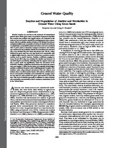
Annual Mean Flow More than twice the amount of streamflow entered the bay in 2003 than in 2002 (fig. 3). This was the third highest amount since 1937 when the USGS began keeping records to compute estimates of the total streamflow to the bay. These computation methods are described in Bue (1968). Between 1940 and 1959, 15 of the 20 years had annual total streamflow values within the interquartile range (between the 25th and 75th percentiles). A dry period occurred in the 1960s (6 of the 10 years were below the 25th percentile), and wetter conditions occurred in the 1970s (5 of the 10 years were above the 75th percentile). The most variable flows were in the last 10 years, between 1994 and 2003; only 2 years were within the interquartile range. The wetter conditions observed from 1970 to the present (11 of 34 years

10


Table 3. Summary of trend tests, results of evaluations, and suggested approaches used in this report. Type of trend Streamflow Time step Reason for test

Trend test evaluated Result of evaluation

Suggested approach

Concentrations (observed, flow-weighted, flow-adjusted)

Loads

Quarterly, annual Instantaneous, monthly, annual Instantaneous, monthly, annual Variability of streamflow helps to assess Observed concentration gives most direct Changes in load over time help explain changes in tidal waters. changes in water quality in nontidal and measure of water-quality change. tidal waters. Flow-weighted approximates the monthly concentration to help explain changes in the tidal waters.

Linear regression

Flow-adjustment compensates for the influence of streamflow and seasonality and accesses change due to human activities. ESTIMATOR, linear regression Linear regression

Autocorrelation within daily-mean and monthly-mean streamflow time series makes trend estimation difficult.

Potential for bias in trend assessment due to sampling protocols that target higher flows.

Very few statistically significant trends in quarterly-mean and annual-mean streamflow.

Therefore, did not perform trend tests for observed or flow-weighted concentration.

Flow-adjusted concentrations estimated using a revised approach. Develop additional statistical methods to Continue using linear regression for quarterly-mean and annual-mean stream- “remove bias” and improve an approach for trends on observed and flow-weighted flow. concentrations. Consider use of time-series process models for trend estimation.

A trend test for load is based on estimated loads that already have uncertainty. Therefore, a trend in load was discontinued. Potential for bias in trend assessment due to sampling protocols that target higher flows. Develop additional statistical methods to incorporate load uncertainty and improve an approach for trends on loads.

Figure 3. Variation in annual mean flow entering the Chesapeake Bay, 1935-2003, using computations as described in Bue (1968).

Changes in Water Quality were above the 75th percentile), along with the effects of increased nutrients and sediment from human activities, have been cited as one possible cause for the declines in dissolved oxygen and water clarity in the bay that were documented in the 1970s and that remain today (Phillips, 2002). Linear regression models of annual mean streamflow were developed for all 33 sites in this study. Only one site (Choptank River) yielded a statistically significant trend (eqn. 6). ln ( y ) = – 78.5 + 0.04t + ε

(6)

where ln is the natural logarithm function; y is annual-mean streamflow for a particular season, in cubic feet per second; -78.5 is a constant; 0.04 is the coefficient on time and estimates the trend; t is time, in years; and ε is the unexplained noise or error in the data. with R2 = 0.3 and p-value = 0.01. This model indicates a statistically significant increase in annual-mean streamflow, estimated to be approximately 4 percent per year.

Quarterly Mean Flow Changes in quarterly-mean streamflow can provide insight into hydrological changes within a watershed for a particular season and help explain changes in the bay and tidal rivers. Linear regression models were developed for four “seasons” (January-February-March, April-May-June, July-August-September, and October-November-December) for all 33 sites in this study. As is the case for daily-mean and monthly-mean streamflow, autocorrelation within the quarterly-mean streamflow time series for each season makes trend estimation difficult. However, graphical depiction of the seasonal data and some summary statistics can provide insights into variations in flow in the Chesapeake Bay watershed (fig. 4 and Appendix 1). A number of observations are common to all RIM sites. The drought of 1999-2002 is evident for all nine RIM sites, as is the relatively wet 2003. For the three largest rivers (Susquehanna, Potomac, and James, fig. 4), all 12 quarters for 1999 through 2001 were normal (between the 25th and 75th percentiles) or dry (below the 25th percentile). For all nine RIM sites, all four quarters of 2003 exhibited normal or above-normal (above the 75th percentile) flows (fig. 4 and Appendix 1).

Changes in Water Quality Changes in water quality in terms of concentrations and loads are presented for 1985-2003 for most of the sites. Some sites have shorter data-collection periods. Results include summary statistics and trends. Not all trends tests previously used (Langland and others, 1999) are presented based on the evalua-

11

tion of trend procedures. Reasons for omitting specific trends tests are presented and discussed in the section “Study Methods.”

Observed Concentrations The most direct measure of change in water quality is observed-concentration data. The range of observed concentrations of TN, TP, and SED for the 33 water-quality monitoring sites are listed in table 4. TN concentrations were elevated in the northern five river basins (Susquehanna, Choptank, Western Shore, Patuxent, and Potomac Rivers) compared to TN concentrations in the southern five river basins (Rappahannock, Mattaponi, Pamunkey, James, and Appomattox Rivers). The median TN concentrations in the northern five basins ranged from 0.90 to 7.50 mg/L, compared to the median TN concentrations in the southern five basins that ranged from 0.43 to 0.93 mg/L. TP concentrations generally were lower in the five northern basins; the median concentrations ranged from 0.017 to 0.283 mg/L, compared to the median concentrations in the southern five basins that ranged from 0.030 to 0.500 mg/L. SED concentrations in the Susquehanna River Basin were elevated (median range = 13 to 43 mg/L) compared to the remaining nine river basins (median range = 3 to 36). The RIM sites have been established in 9 of the 10 major river basins (in this report) within the Chesapeake Bay watershed. The Western Shore River Basin is the only major basin not represented by the RIM program. The distribution (10th and 90th percentiles) of TN, TP, and SED collected at the nine RIM sites during 1985-2003 is shown in figure 5. TN concentrations generally were elevated at the Susquehanna, Potomac, Patuxent, and Choptank RIM sites, compared to the concentrations observed at the Rappahannock, Mattaponi, Pamunkey, James, and Appomattox RIM sites. The James and Rappahannock River RIM sites exhibited the greatest variability in observed TN concentration. TP concentrations at each of the nine RIM sites typically ranged from 0.06 to 0.07 mg/L. The greatest variability in TP concentration was observed at the Patuxent, Rappahannock, and James RIM sites. Sediment concentrations also were similar at each of the nine RIM sites and typically ranged from 4 to 100 mg/L. The Rappahannock and James RIM sites exhibited the greatest variability in observed sediment concentration. Annual distribution of observed TN, TP, and SED concentrations collected at the RIM stations for the three largest basins (Susquehanna, Potomac, and James Rivers) in the Chesapeake Bay watershed is shown in figures 6A, B, and C. These figures include the 10th and 90th data percentiles with “outliers” (data points 1.5 times outside the interquartile range) to provide a full distribution of the data by site. Annual distribution for each of these three constituents collected at the remaining six RIM sites are presented in Appendix 2. The primary concern regarding water quality within the Chesapeake Bay watershed over the past 5 years is to what extent water quality was influenced by the extreme variability in flow conditions. The 4-year period, 1999-2003, was dominated by drought conditions; 2003 was one of the wettest years on record (fig. 3). TN concentrations at

12


Figure 4. Quarterly mean streamflow for the Susquehanna (1985-2003), Potomac (1985-2003), and James (1989-2003) Rivers. For each season, 25th, 50th, and 75th percentiles were calculated. Bars representing the quarterly mean flow are red if the value for that quarter is below the 25th percentile, blue if above the 75th percentile, and black if between the 25th and 75th percentiles.

Table 4. Minimum, mean, median, and maximum concentrations of total nitrogen, total phosphorus, and suspended sediment at the 9 River Input Monitoring sites and 25 MultiAgency Nontidal Program sites in the Chesapeake Bay watershed. [Station: Map site number, location on figure 1; Flow, USGS streamflow-gaging station number; WQ, water-quality site alphanumeric identity; POR: Sample period of record for statistical determination; Statistics: mg/L, milligrams per liter; Number of samples, samples used in the statistical determination; Min, minimum; Med, median; Max, maximum]

Station

Statistics Total nitrogen as N (mg/L)

Flow

WQ

Map site Drainage numarea ber

POR

Number of samples

Min

Med

Mean

Total phosphorus as P (mg/L)

Max

Number of samples

Suspended sediment / solids (mg/L)

Min

Med

Mean

Max

Number of samples

Min Med

Mean

Max

Susquehanna River Basin 01531500

01531500

1

7,797

1988-2003

472

0.00

1.12

1.19

4.30

519

0.013

0.068

0.093

0.700

1

519

0

27

88

2,226

01540500

01540500

2

11,220

1984-2003

585

.21

1.24

1.34

6.20

656

.010

.070

.099

.730

1

650

0

30

78

1,230

01553500

01553500

3

6,850

1984-2003

538

.00

1.04

1.12

6.73

610

.009

.040

.061

.880

1 604

1

15

55

1,531

01567000

01567000

4

1984-2003

461

.44

1.80

1.87

11.46

524

.003

.079

.109

6.300

1

518

0

17

45

687

1 618

3,354

01576000

01576000

5

25,990

1986-2003

548

.73

1.60

1.71

7.92

622

.006

.080

.106

.520

1

43

76

1,117

01576754

01576754

6

470

1984-2003

539

1.23

7.50

7.73

30.00

590

.030

.283

.364

4.200

1

608

0

41

125

8,710

01578310

01578310

7

27,100

1984-2003

563

.81

1.70

1.75

6.60

586

.010

.045

.055

.320

1

575

1

13

27

863

435

.007

.065

.078

.330

1

423

1

7

14

161

217

.010

.028

.048

.503

2

223

0

5

18

1,502

220

.010

.033

.044

.950

2

222

0

6

8

39

551

3

36

66

740

Choptank River Basin 01491000

01491000

8

113

1984-2003

425

.64

1.70

1.69

3.58

Western Shore River Basin 01586000

NPA0165

9

56.6

1985-2003

217

1.66

4.25

4.22

6.30

Patuxent River Basin 01592500 01594440

PXT0809 01594440

10 11

132 348

1985-2003 1984-2003

217 554

.02 1.13

1.64 2.20

1.67 2.63

3.70 8.40

631

.004

.140

.183

1.200

1

214

.010

.047

.079

1.100

2

Potomac River Basin 01599000

GEO0009

12

72.4

1985-2003

206

.49

1.50

1.52

4.43

216

0

16

25

370

WIL0013

13

247

1985-2002

184

.20

1.07

1.15

2.55

190

.010

.017

.033

.382

1

6

14

240

01610000

POT2766

14

3,109

1985-2003

197

.40

1.06

1.10

2.25

195

.010

.036

.050

.730

2

193

0

6

14

364

01613000

POT2386

15

4,073

1985-2003

210

.40

1.01

1.09

4.60

213

.010

.035

.053

.397

2

220

0

5

14

336

01614500

CON0180

16

501

1985-2003

208

.87

4.65

4.67

7.60

214

.010

.125

.154

.741

2

220

0

7

19

425

01626000

1BSTH027.85

17

127

1984-2003

181

.36

.90

.93

3.49

184

.010

.100

.099

.400

2

189

1

5

8

56

01631000

1BSSF003.56

18

1,642

1984-2003

182

.37

1.42

1.54

22.70

184

.010

.100

.163

4.000

2

188

0

5

9

148

01634000

1BNFS010.34

19

768

1984-2003

178

.35

1.95

2.09

32.60

180

.060

.100

.155

.720

2

180

0

3

12

311

01638500

POT1595

20

9,651

1985-2003

216

.82

2.05

2.07

4.96

215

.010

.060

.088

2.900

2 225

0

8

20

784 255

MON0155

21

01646000

1ADIF000.86

22

01646580

PR01

23

817 57.9 11,570

1985-2003

211

1.28

3.62

3.63

7.60

214

.015

.166

.218

1.200

0

9

19

1984-2003

171

.24

1.44

2.59

20.40

174

.010

.100

.146

9.400

2

178

1

5

19

262

1984-2003

913

.35

1.72

1.79

5.09

931

.010

.070

.096

1.390

2

199

1

11

73

2,994

13

01643000

2 223

Changes in Water Quality

01601500

2 189

14

Table 4. Minimum, mean, median, and maximum concentrations of total nitrogen, total phosphorus, and suspended sediment at the 9 River Input Monitoring sites and 25 MultiAgency Nontidal Program sites in the Chesapeake Bay watershed.—Continued

Station

Statistics Total nitrogen as N (mg/L)

Map site Drainage numarea ber

Total phosphorus as P (mg/L)

Number of samples

Min

Med

1984-2003

166

0.24

0.81

0.83

1.81

1,596

1988-2003

512

.12

.93

1.07

4.21

28

601

1989-2003

549

.22

.57

8-NAR005.42

26

463

1984-2003

190

.15

.43

.43

01673000

01673000

27

1,081

1989-2003

566

.31

.69

.74

02013100

2-JKS023.61

29

614

1984-2003

205

.24

.75

.79

02026000

2-JMS229.14

30

3,683

1984-2003

185

.15

.59

02029000

2-JMS189.31

31

4,584

1984-2003

171

.14

.52

Flow

WQ

01666500

3ROB0001.90

24

179

01668000

01668000

25

01647500

01674500

01671020

POR

Number of samples

Suspended sediment / solids (mg/L)

Min

Med

Mean

Max

Number of samples

168

0.200

0.100

0.102

0.700

2 172

1

5

12

198

521

.006

.055

.138

1.500

2 521

1

16

83

972

557

.010

.050

.057

.392

2 573

1

6

10

261

.94

193

.010

.030

.055

.220

2 193

0

3

5

95

2.58

568

.020

.071

.088

.802

2 585

1

14

32

347

1.81

207

.040

.500

.887

6.500

2 207

1

5

7

24

.64

1.77

188

.030

.100

.186

.960

2 190

1

5

13

233

.54

1.50

174

.020

.100

.140

.600

2 179

1

5

13

244

2

575

1

31

81

800

2 557

1

8

11

70

Mean

Max

Min Med

Mean

Max

Rappahannock River Basin

Mattaponi River Basin .59

1.88

Pamunkey River Basin

James River Basin

02035000

02035000

32

6,257

1988-2003

569

.05

.64

.78

3.30

571

.009

.114

.168

1.400

.010

.047

.053

.200

Appomattox River Basin 02041650

02041650

33

1,344

1989-2003

549

.15

.57

.60

1.35

1Suspended-sediment

concentration was determined through the suspended sediment concentration analysis.

2Suspended-sediment

concentration was determined through the suspended solid concentration analysis.

554


[Station: Map site number, location on figure 1; Flow, USGS streamflow-gaging station number; WQ, water-quality site alphanumeric identity; POR: Sample period of record for statistical determination; Statistics: mg/L, milligrams per liter; Number of samples, samples used in the statistical determination; Min, minimum; Med, median; Max, maximum]


15

Figure 5. Range in observed concentrations for the nine River Monitoring Input sites, Chesapeake Bay watershed, 1985-2003.

16


Figure 6A. Annual distribution of observed total nitrogen, total phosphorus, and sediment concentrations collected at the River Input Monitoring sites for the Susquehanna River in the Chesapeake Bay watershed, 1984-2003.


Figure 6B. Annual distribution of observed total nitrogen, total phosphorus, and sediment concentrations collected at the River Input Monitoring sites for the Potomac River in the Chesapeake Bay watershed, 1984-2003.—Continued

17

18


Figure 6C. Annual distribution of observed total nitrogen, total phosphorus, and sediment concentrations collected at the River Input Monitoring sites for the James River in the Chesapeake Bay watershed, 1984-2003.—Continued

Changes in Water Quality the three major RIM sites generally exhibited decreased concentrations during the 1999-2002 drought period. Conversely, TN concentration increased markedly in 2003 as a result of the prolonged high-flow conditions. TP concentrations at the Susquehanna RIM site exhibited a similar pattern to what was observed for TN concentration (fig. 6A) with decreased concentrations during the drought and markedly elevated concentrations during the prolonged high-flow period. The Potomac and James River RIM sites (figs. 6B and 6C) did not exhibit any distinguishing patterns during the drought and prolonged highflow periods. The sediment concentrations at the Potomac and James River RIM sites had drastically different concentrations when comparing the last year of the drought (2002) to the extended high-flow period (2003). SED concentrations observed during 2002 at both of these RIM sites were collectively one of the lowest on record; 2003 yielded considerably elevated concentrations. The Susquehanna RIM site exhibited a similar, but less variable, pattern as what was observed at the Potomac and James RIM sites with respect to SED concentration. This attenuated pattern observed at the Susquehanna RIM site was related to sediment settling in the three reservoirs above the monitoring site. The prolonged high-flow conditions and elevated concentrations of TN, TP, and SED, in 2003, resulted in one of the largest annual loads of TN, TP, and SED delivered to the Chesapeake Bay since monitoring began in the late 1980s.

Flow-Weighted Concentration An approach to evaluating the changing relation between streamflow and load is a FWC. It approximates the annual concentration. Changes over time can be illustrated within a basin and comparisons made among different basins. The Potomac River consistently had higher annual TN FWC averaging about 2.25 mg/L (fig. 7). This exceeded the FWC in the Susquehanna (1.71 mg/L) and was about three times the annual FWC of TN in the James River (0.75 mg/L). The FWC for TN in the Susquehanna River decreased from 1988 to 1998, with a more pronounced decline in the drought years of 1999-2002, and then increased in 2003. In general, the TN FWC for the Potomac and James Rivers exhibited little change from 1988 through 2003 except during the past 5 years, first dropping from 1999 through 2002 because of drought conditions over most of the bay watershed, then increasing in 2003 because of above-normal precipitation over the bay watershed. FWC for TP and SED exhibited much more variability than TN because of different mechanisms of transport (fig. 7). Most of the TN is transported in the dissolved phase as nitratenitrogen; TP and SED are transported in the particulate phase. From 1988 to 2003, the TP FWC averaged about 0.15 mg/L for the Potomac and James Rivers, and the Susquehanna River averaged about 0.05 mg/L. The lower value in the Susquehanna River was most likely because of the phosphorus and sediment trapping behind three large reservoirs in the lower reaches of

19

the river. Figure 7 suggests an increase in TP FWC even through the drought period of 1999-2002 for all three major rivers. As with TP, the average SED FWC during 1988-2003 was similar at the Potomac and James Rivers (120 mg/L and 85 mg/L, respectively) and lowest for the Susquehanna River (25 mg/L), likely because of the settling and trapping of sediment behind the three reservoirs. The variability in FWC was consistent among the major rivers (fig. 7), with the exception of the Potomac River in 2002. The FWC increased by a factor of 10 from 2001 to 2002 with little change in flow, then was reduced by half in 2003 when flow increased by a factor of 4.

Flow-Adjusted Concentration The observed and FWC data are highly influenced by changes in streamflow. Therefore, the USGS attempted to compensate for the influence of streamflow to improve understanding of changes in water quality that result from human influences. Results from ESTIMATOR are used to determine a flow-adjusted trend for concentration, by partitioning variability in observed concentration data due to season and flow, so that the coefficient from the “time” parameter is an estimate of the amount of change over time. An important point to mention is that the results of “flow adjustment” do not necessarily represent all the changes in water quality that result from human influence and management actions, only those apart from flow. For example, a change in farming practices that reduces surface runoff but increases ground-water recharge and a change in atmospheric deposition will not be captured using flow adjustment. Therefore, while FAC trends are an indicator of human activities affecting water quality within a watershed, the relative magnitude must be considered in terms of the hydrologic variability. For the period 1985-2003, results from ESTIMATOR indicated about 55 percent of the sites (17 of 33 sites) had decreasing flow-adjusted trends for TN (fig. 8 and Appendix 3). Four sites indicated increasing trends; the remaining 12 sites did not have any significantly detectable trend. All seven sites in the Susquehanna River Basin had decreasing trends in TN. In the Potomac River Basin, there were nine decreasing trends, two increasing trends, and one site with no detectable trend. Sites in the James River Basin indicated no significantly detectable trends. Trends in nitrate concentration adjusted for flow were decreasing at 18 sites, occurring in nearly all major Chesapeake Bay drainage basins, and increasing at 5 of the 33 sites (Appendix 3). Decreasing trends for TN and nitrate coincided at 14 sites; increasing trends coincided at 2 sites. Flow-adjusted trends for TP concentrations were significantly decreasing at 25 of the 33 sites (fig. 9 and Appendix 3) and increasing at 4 sites; the remaining 4 sites did not have any significantly detectable trends. Trends were decreasing at 4 RIM sites with decreasing trends in TP occurring in 8 of the 10 major bay drainage basins. Increasing trends in TP were identified at four sites, three of which are RIM sites.

20


Figure 7. Flow-weighted concentrations for the Susquehanna, Potomac, and James Rivers entering the Chesapeake Bay for 1988-2003.


Figure 8. Trends in flow-adjusted concentrations for total nitrogen, Chesapeake Bay watershed, 1985-2003.

21

22


Figure 9. Trends in flow-adjusted concentrations for total phosphorus, Chesapeake Bay watershed, 1985-2003.

Changes in Water Quality Significant downward flow-adjusted trends for SED concentration were detected at 15 sites. Four RIM sites indicted downward trends. An upward trend was reported at two sites (sites 26 and 27) (fig. 10 and Appendix 3). The RIM sites had four increasing and one decreasing trend in SED. The Susquehanna River Basin indicted decreasing trends at all seven sites. Results for the Potomac Basin indicate about an equal number of decreasing (7) trends and no significantly detectable trends (8). In the James River Basin (including the Appomattox Basin), there was one decreasing trend, and four sites had no significantly detectable trends. The significance and range in magnitude for TN, TP, and SED for concentrations adjusted for flow for the nine RIM sites are shown in figure 11. Five sites did not have significant FAC trends for TN. The Susquehanna, Potomac, and Patuxent Rivers had decreasing trends (improvement) of -28, -13, and -56 percent, respectively; the Pamunkey River increased 23 percent (fig. 11 and Appendix 3). TP trends adjusted for flow decreased at four rivers, ranging from -62 to -25 percent, and increased at three sites, ranging from 26 to 65 percent. Four RIM sites had decreasing FAC trends for SED, ranging from -65 to -27 percent, and a 53 percent increasing FAC trend for SED at one site. In summary, for the nine RIM sites, there were 16 significant trends and 13 no significantly detectable trend results for TN, TP, and SED. Thirteen of the 16 had significant trends greater than a 25-percent change in magnitude. As previously mentioned, streamflows for the years 19992002 were below normal; streamflow for most of 2003 was well above normal throughout most areas of the Chesapeake Bay watershed. Trends at the nine RIM sites for TN, TP, and SED ending in calendar years 2002 and 2003 were examined to determine if the extreme change in hydrology affected the FAC trends. The extreme variability in hydrology did not affect the significance or direction of trend at four of the nine RIM sites (Susquehanna, Patuxent, Potomac, and Pamunkey Rivers) (fig. 1 and table 5). Three sites were consistently decreasing for TN, TP, and SED; one site (Pamunkey River) was consistently increasing for TN, TP, and SED. A significant change occurred at five RIM sites; Choptank and James Rivers for TN, Rappahannock River for TP, and Mattaponi and Appomattox Rivers for SED (table 5).

Loads Nutrient and sediment loads have a large impact on the health of the Chesapeake Bay Ecosystem and habitat in the rivers of the watershed. In 2003, nutrient and sediment loads at the RIM sites were the second highest since 1990. The estimated loads at the nine RIM sites for 2003 were 350 million pounds (Mlbs) of nitrogen, 30 Mlbs of phosphorus, and 18,200 Mlbs of sediment. The loads at the RIM sites represented about 60 percent of the total load that entered the tidal waters of the bay watershed (Gary Shenk, U.S. Environmental Protection Agency, written commun., 2004). The increased nutrient and sediment loads probably resulted in less light penetration in the

23

bay waters, which may have contributed to a decline of submerged aquatic vegetation (SAV). The increased nutrient loads also may have contributed to large areas of low dissolved oxygen levels in the bay during the summer of 2003. The prolonged high-flow conditions and elevated concentrations of TN, TP, and SED, in 2003, resulted in one of the greatest annual loads of TN, TP, and SED delivered to the Chesapeake Bay since monitoring began in the late 1980s. In 2003, more than twice the amount of river flow entered the bay than in 2002 (fig 12). This was the third highest amount of river flow to enter the bay since 1937 (fig. 3), when the USGS began keeping records to compute estimates of the total flow to the bay. The large increase in river flow was one factor that contributed to the loads in 2003 being much higher than 2002. At the RIM sites, about 3 times the amount of TN, 5 times the amount of TP, and 11 times the amount of SED entered the bay in 2003 compared to 2002. In addition to higher streamflow, the loads also were influenced by higher nutrient and sediment concentrations at the RIM sites in 2003 than in 2002. The increased TN concentrations were the result of higher amounts of nitrogen being flushed from the land and ground water. Increased SED and TP concentrations were caused by the substantial erosion of sediment from the land and streams. A more detailed description of the concentrations in each river is shown in figure 5 and in table 4. The large variability of loads since 1985 contributed to the difficulty in attempting to detect significant trends over time. As previously mentioned, because of the concerns of using any estimated load to access a trend, no trends in loads are reported this year. Alternative methods of expressing a change in load with time (trend) are being explored. Trends in load may be reinstated in the future, pending the development of additional statistical methods.

24


Figure 10. Trends in flow-adjusted concentrations for sediment, Chesapeake Bay watershed, 1985-2003.


Figure 11. Significance and range in magnitude in trend for flow-adjusted concentrations from the ESTIMATOR model for the nine River Input Monitoring sites, Chesapeake Bay watershed, 1985-2003.

25

26


Figure 12. Combined annual flow and total nitrogen, total phosphorus, and sediment load for the nine River Input Monitoring sites flowing into the Chesapeake Bay for 1990-2003.

Summary and Conclusions

27

Table 5. Significant (flow-adjusted concentration) trend direction for the above-normal streamflow in 2003 (1985-2003 trends) and belownormal streamflow in 2002 (1985-2002 trends) calendar years. [ns; no significant trend detected]

Basin Choptank Susquehanna Patuxent Potomac Rappahannock Pamunkey Mattaponi James Appomattox

Site number

Total nitrogen

Total phosphorus

Sediment

Site ID (fig. 1)

2003

2002

2003

2002

2003

2002

8 7 11 23 25 27 28 32 33

ns decrease decrease decrease ns increase ns ns ns

decrease decrease decrease decrease ns increase ns decrease ns

increase decrease decrease increase decrease increase ns decrease ns

increase decrease decrease increase ns increase ns decrease ns

decrease decrease decrease decrease ns increase ns ns ns

decrease decrease decrease decrease ns increase increase ns increase

01491000 01578310 01594440 01646580 01668000 01673000 01674500 02035000 02041650

Summary and Conclusions Nutrient and suspended sediment data from 33 sites in nontidal parts of the Chesapeake Bay Basin were analyzed to document changes in streamflow, concentrations, and loads from 1985 through 2003, as part of an annual update of waterquality conditions for the Chesapeake Bay Program. Annual loads and flow-adjusted concentration (FAC) trends were estimated by use of the U.S. Geological Survey (USGS) ESTIMATOR model. Changes in seasonal and annual flow, annual nutrient and sediment concentrations and loads, and flow-weighted concentration (FWC) were evaluated to help assess impacts on the bay ecosystem. FAC trends were evaluated to help assess changes that result from human activities and management actions. As part of this report, several different trend techniques were evaluated to improve statistical analysis to help address changes in water quality and assess the influence of management actions in reducing nutrient and sediment concentrations. Streamflow in 2003 was more than double that of 2002 and was the third highest since 1937. However, the results for streamflow data for 1985 through 2003 revealed a significant increase in annual flow for only one site, Choptank River in Maryland. Streamflow changes for the remaining 32 sites were not statistically significant because of serial correlation for daily, monthly, seasonal, and annual trends. Observed concentration samples collected for 10 major river basins indicate higher ranges in total-nitrogen concentrations in the five “northern” basins in Pennsylvania and Maryland compared to the five “southern” basins in Virginia. Totalphosphorus concentrations showed no distinct difference among the 10 basins. The median range of sediment concentrations was highest in the Susquehanna. Median concentrations increased at all nine River Input Monitoring (RIM) sites for total nitrogen, total phosphorus, and sediment in 2003 compared to 2002. A test for trend in observed concentration was not performed because of concerns that sampling protocols may have biased the trend because a disproportionate number of samples were collected during high-flow conditions.

The Potomac River consistently had higher FWC for annual total nitrogen averaging about 2.25 mg/L, nearly double that of the Susquehanna River and three times that of the James River. The Potomac generally exhibited little change except during the past 5 years, as a result of drought conditions from 1999 through 2002 and well above-normal streamflow conditions in 2003. FWC values for total phosphorus averaged about 0.15 mg/L for the Potomac and James Rivers and 0.05 mg/L for the Susquehanna River. The lower FWC value in the Susquehanna River is likely because of the sediment- and phosphorustrapping capability of three large reservoirs in the lower reaches of the river. An increase in total phosphorus FWC was observed for all three major rivers through the drought period of 19992002. FWC for sediment was similar at the Potomac and James Rivers (120 and 85 mg/L, respectively) and lowest for the Susquehanna River (25 mg/L) because of the settling and trapping of sediment behind the three reservoirs. The variability in annual FWC for sediment is consistent among the major rivers with the exception of the Potomac River in 2002 when the FWC increased by a factor of 10 with little change in flow, then was reduced by half in 2003 when flow increased. In 2003, nutrient and sediment loads at the RIM sites were the second highest since 1990. In 2003, the loads at the nine RIM sites were 350 million pounds (Mlbs) of nitrogen, 30 Mlbs of phosphorus, and 18,200 Mlbs of sediment. The loads at the RIM sites represented about 60 percent of the total load that entered the tidal waters of the bay watershed. The nutrient and sediment loads in 2003 were influenced by near-record river flow to the bay in 2003 when more than twice the amount of river flow entered the bay than in 2002. This was the third-highest amount of river flow to enter the bay since 1937 when the USGS began keeping records to compute estimates of the total flow to the bay. The large increase in river flow contributed about 3 times the amount of nitrogen, 5 times the amount of phosphorus, and 11 times the amount of sediment entering the bay in 2003 compared to 2002 at the RIM sites. The nutrient and sediment loads in 2003 contributed to low dissolved oxygen and loss of submerged aquatic vegetation (SAV) in 2003.

28


When the influences of flow and seasonality are removed, results for trends adjusted for flow (FAC) suggest improvement in water quality due to management actions. Results indicated about 55 percent of the sites (18 sites) had decreasing FAC for total nitrogen. Four sites indicated increasing FAC trends, with no significantly detectable trends at the remaining 11 sites. Trends were deceasing at four and increasing at one of the nine RIM sites. All seven sites in the Susquehanna River Basin had decreasing FAC trends in total nitrogen. In the Potomac River Basin, there were nine sites with decreasing trends and two sites with increasing FAC trends; the James River Basin had one site with a decreasing trend and four sites showed no significantly detectable FAC trends. FAC trends in nitrate concentration were decreasing at 18 sites in nearly all major Chesapeake Bay drainage basins and increasing at 5 of the 33 sites. FAC trends in total phosphorus were significantly decreasing at 25 of the 33 sites, increasing at 4 sites, with no significantly detectable trends at the remaining 4 sites. Trends were decreasing at 4 RIM sites with decreasing trends in total phosphorus in 8 of the 10 major bay drainage basins. Increasing trends in total phosphorus were identified at four sites, three of which are RIM sites. Significant downward FAC trends for suspended sediment were detected at 15 sites. Four RIM sites indicated downward FAC trends. An upward trend was reported at three sites. For FAC trends in sediments, four of the RIM sites showed an increasing trend and one showed a decreasing trend. All seven sites in the Susquehanna River Basin indicated a decreasing trend. Results for the sites in the Potomac River Basin indicate about an equal number of decreasing (7) trends and no significantly detectable trends (8). At the James River Basin sites, there was one decreasing trend and four no significantly detectable FAC trends. As part of an evaluation of current trend methodology, trends in estimated loads in any time series (annual, monthly, or using the loads in the flow weighted concentrations) from the ESTIMATOR model are not reported because of concerns the load estimates in the time series are not independent, are estimates rather than measurements, and may not be representative of the variability of the natural system. Estimating trend on the estimates of load may produce biased results. In addition, there is concern over the potential bias introduced from the targeted sampling protocols used at the RIM sites. Although targeting higher flow events to estimate loads is appropriate for load estimation using models similar to ESTIMATOR, this targeting could possibly bias a simple linear regression analysis trend. The reporting of these trends may be reinstated in the future pending the development of additional statistical methods.

Acknowledgments The authors wish to thank all who participated in the writing, reviewing, and revisions made to this report. In particular, a special thanks goes to Greg Schwarz and Jurate Landwehr for their insightful statistical reviews and suggestions. In addition, thanks to the USGS reports section staff for their prompt revisions, editorial, and publishing assistance.

References Cited Box, G.E.P., and Jenkins, G.M., 1976, Time series analysis—Forecasting and control (revised edition): Englewood Cliffs, N.J., Prentice-Hall, 575 p. Bradu, D., and Mundlak, Y., 1970, Estimation in log-normal linear models: Journal of the American Statistical Association, v. 65, no. 329, p. 198-211. Bue, C.D., 1968, Monthly surface-water input to Chesapeake Bay: U.S. Geological Survey Open File Report 68-29, 45 p. Cohn, T.A., 1988, Adjusted maximum likelihood estimation of the moments of lognormal populations from type 1 censored samples: U.S. Geological Survey Open-File Report 88-350, 34 p. Cohn, T.A., Caulder, D.L., Gilroy, E.J., Zynjuk, L.D., and Summers, R.M., 1992, The validity of a simple log-linear model for estimating fluvial constituents loads—An empirical study involving nutrient loads entering Chesapeake Bay: Water Resources Research, v. 28, no. 9, p. 2,353-2,364. Cohn, T.A., DeLong, L.L., Gilroy, E.J., Hirsch, R.M., and Wells, R.M., 1989, Estimating constituent loads: Water Resources Research, v. 25, no. 5, p. 937-942. Darrell, L.C., Majadi, B.F., Lizarraga, J.S., and Blomquist, J.D., 1998, Nutrient and suspended-sediment concentrations, trends, loads, and yields, from the nontidal part of the Susquehanna, Potomac, Patuxent, and Choptank Rivers, 198596: U.S. Geological Survey Water-Resources Investigations Report 98-4177, 38 p. Gilroy, E.J., Hirsch, R.M., Kirby, W.H., and Cohn, T.A., 1990, Mean square error of regression-based constituent transport estimates: Water Resources Research, v. 26, no. 9, p. 2,0692,077. Helsel, D.R., and Hirsch, R.M., 1992, Statistical methods in water resources: Amsterdam, Elsevier Science Publishers, Studies in Environmental Science, v. 49, 522 p. Kammerer, P.A., Garn, H.S., Rasmussen, P.W., and Ball, J.R., 1998, A comparison of water-quality sample collection methods used by the U.S. Geological Survey and the Wisconsin Department of Natural Resources in Proceedings of the National Water-Quality Monitoring Council, National Conference on Monitoring, July 7-9, 1998, Reno, Nev.: Washington D.C., U.S. Environmental Protection Agency, p. III-259-269. Langland, M.J., Blomquist, J.D., Sprague, L.A., and Edwards, R.E., 1999, Trends and status of flow, nutrients, and sediments for selected nontidal sites in the Chesapeake Bay Watershed, 1985-98: U.S. Geological Survey Open-File Report 99-451, 46 p. Montgomery, D.C., and Peck, E.A., 1982, Introduction to linear regression analysis: New York, John Wiley and Sons, Inc., 504 p. Phillips, S.W., ed., 2002, The U.S. Geological Survey and the Chesapeake Bay—The role of science in environmental restoration: U.S. Geological Survey Circular 1220, 32 p. U.S. Environmental Protection Agency, 2003, Ambient water quality criteria for dissolved oxygen, water clarity, and chlorophyll a for the Chesapeake Bay and its tidal tributaries: 903-R-03-002, 231 p.

Appendix 1

Figure 1.1. Quarterly-mean streamflow for the Choptank River and Patuxent River, 1985-2003. Figure 1.2. Quarterly-mean streamflow for the Appomattox, Rappahannock, Pamunkey, and Mattaponi Rivers, 1990-2003.

30

Changes in Flow and Water Quality in Selected Nontidal Sites in the Chesapeake Bay Basin, 1985-2003

Figure 1.1. Quarterly mean streamflow for the Choptank River and Patuxent River, 1985-2003. For each season, 25th, 50th, and 75th percentiles were calculated. Bars representing the quarterly mean flow are red if the value for that quarter is below the 25th percentile, blue if above the 75th percentile, and black if between the 25th and 75th percentiles.

Appendix 1 31

Figure 1.2. Quarterly mean streamflow for the Appomattox, Rappahannock, Pamunkey, and Mattaponi Rivers, 19902003. For each season, 25th, 50th, and 75th percentiles were calculated. Bars representing the quarterly mean flow are red if the value for that quarter is below the 25th percentile, blue if above the 75th percentile, and black if between the 25th and 75th percentiles.

Appendix 2 Figure 2.1 - Statistical summaries for water-quality concentration data for total nitrogen (A), total phosphorus (B), and sediment (C) for the Choptank River. Figure 2.2 - Statistical summaries for water-quality concentration data for total nitrogen (A), total phosphorus (B), and sediment (C) for the Patuxent River. Figure 2.3 - Statistical summaries for water-quality concentration data for total nitrogen (A), total phosphorus (B), and sediment (C) for the Rappahanock River. Figure 2.4 - Statistical summaries for water-quality concentration data for total nitrogen (A), total phosphorus (B), and sediment (C) for the Mattaponi River. Figure 2.5 - Statistical summaries for water-quality concentration data for total nitrogen (A), total phosphorus (B), and sediment (C) for the Pamunkey River. Figure 2.6 - Statistical summaries for water-quality concentration data for total nitrogen (A), total phosphorus (B), and sediment (C) for the Appomattox River.

34


Figure 2.1. Statistical summaries for waterquality concentration data for total nitrogen (A), total phosphorus (B), and sediment (C) for the Choptank River.

Appendix 2 35

Figure 2.2. Statistical summaries for waterquality concentration data for total nitrogen (A), total phosphorus (B), and sediment (C) for the Patuxent River.

36


Figure 2.3. Statistical summaries for waterquality concentration data for total nitrogen (A), total phosphorus (B), and sediment (C) for the Rappahannock River.

Appendix 2 37

Figure 2.4. Statistical summaries for waterquality concentration data for total nitrogen (A), total phosphorus (B), and sediment (C) for the Mattiponi River.

38


Figure 2.5. Statistical summaries for waterquality concentration data for total nitrogen (A) total phosphorus (B), and sediment (C) for the Pamunkey River.

Appendix 2 39

Figure 2.6. Statistical summaries for waterquality concentration data for total nitrogen (A), total phosphorus (B), and sediment (C) for the Appomattox River.

Appendix 3 Figure 3.1. Location and site number for the 33 sites used in this study, Chesapeake Bay Basin. Station: Site number, location on figure 1; Flow, USGS streamflow gage number; WQ, water-quality site alphanumeric identity. POR:

BegDate, begin date; End Date, end date.

Parameter: Flow, streamflow; TN, total nitrogen; DN, dissolved nitrogen; DNH4, dissolved ammonia; TNH4, total ammonia; TNO3, DNO3, total or dissolved nitrate; TNO3+2, DNO3+2, total or dissolved nitrite plus nitrate; DKJD, dissolved ammonia plus organic nitrogen; TKJD, total ammonia plus organic nitrogen; TP, total phosphorus; DP, dissolved phosphorus; DIP, dissolved inorganic phosphorus; TSS, total suspended solids; SED, suspended sediment. Statistics: Slope, regression slope; P-value, measure of significance of regressor at 0.05; direction, improving (improvement in WQ), degrading (degrading of WQ); ns (no significantly detectable trend); magnitude, LowCI (lower confidence interval), trend (actual estimated trend), UpCI (upper confidence interval); remarks, not normally distributed residuals (nn); >50% BDL, greater than 50 percent below detection limit.

42


Figure 3.1. Location and site number for the 33 sites used in this study, Chesapeake Bay Basin.

Appendix 3. Trends in flow-adjusted concentration data for 9 River Input Monitoring Program sites and 24 Multi-Agency Nontidal Program sites in the Chesapeake Bay Watershed, 1985-2003. [

Changes in Streamflow and Water Quality in ... - Semantic Scholar

Changes in Streamflow and Water Quality in ... - Semantic Scholar

Suggest Documents

Changes in Streamflow and Water Quality in Selected Nontidal Sites ...

Detection of changes in streamflow series in ... - Semantic Scholar

Changes in Streamflow Dynamics in the Rhine ... - Semantic Scholar

Seasonal changes of water quality in a tropical ... - Semantic Scholar

changes in the lower drava river water quality ... - Semantic Scholar

Comparison of SWAT Streamflow and Water Quality in ... - Springer Link

Streamflow, Water Quality, and Aquatic Macroinvertebrates of ...

Dynamic changes in water and salinity in saline ... - Semantic Scholar

environmental water quality assessment in ... - Semantic Scholar

Changes in Biomass and Quality of Alpine Steppe ... - Semantic Scholar

Changes in aberrations and retinal image quality ... - Semantic Scholar

sleep quality changes in insomniacs and non ... - Semantic Scholar

Changes of streamflow in Poyang Lake Basin

Effects of land use changes on streamflow ... - Semantic Scholar

Remote Sensing of Soil and Water Quality in ... - Semantic Scholar

Identification of water quality changes in a water systemâlimitations ...

Surface Water Quality - Semantic Scholar

Water Quality Monitoring - Semantic Scholar

Ground Water Quality - Semantic Scholar

Effects of seasonality on streamflow and water quality ... - Springer Link

Streamflow and water quality of the Grand Calumet River, Lake ...

Comparison of streamflow and water-quality data collection ...

Comparison of streamflow and water-quality data collection

How Do Changes in Water Quality and Dialysate

Changes in Streamflow and Water Quality in ... - Semantic Scholar