Changing range genetic algorithm for multimodal function optimization Adil Amirjanov 1 and Konstantin Sobolev 2 1 Department
of Computer Engineering, Near East University, Nicosia, N. Cyprus; E-mail:
[email protected] 2 Department of Civil Engineering and Mechanics, University of Wisconsin-Milwaukee, Milwaukee, USA E-mail:
[email protected]
Abstract The performance of a sequential changing range genetic algorithm (SCRGA) is described. This algorithm enables the transformation of an unconstrained numerical optimization problem to a constrained problem by implementing constraints which convert the area near previously found optima to an infeasible region. This SCRGA feature is used for locating all optima of unconstrained and constrained numerical optimization problems. Several test cases, related to unconstrained and constrained numerical optimization problems, demonstrate the ability of this approach to reduce the computational costs, significantly improving success rates, accurately and precisely locating all optimal solutions. Keywords:
non-linear programming; genetic algorithms; optimization methods; computational cost
1. Introduction The global numerical optimization problem (GOP) is to find an optimizer x * such that f ( x * ) min f (x) , where x x1 ,, xn R n . The objective function f is defined by the search space S R n , which is the finite interval region on the n -dimensional Euclidean space bounded by the parametric ranges xi xi xi i {1,, n} ( x i is a lower bound and xi is an upper bound of a parameter xi respectively). The search space in GOP is more restricted to a feasible region ( F , where F S ) by a set of constraints g j (x) 0 j {1,, m} .
There are two types of optimization: multi-objective optimization and multimodal optimization. Both types require finding multiple (near-) optimal solutions before making a decision regarding the optimum. For multimodal optimization, the diversity of solutions across the space of variables is desired, while for multi-objective optimization diversity is required in the objective space. Multimodal optimization aims on finding all numerous optima without being constrained by a single optimum. Engineering optimization problems are often classified as multimodal optimization problems. They present the multiple optima in the feasible space of variables. In chemical engineering, it is known that non-isothermal catalyst pellets exhibit multiple steady states; therefore designing non-isothermal catalyst pellets requires finding all solutions of the steady state 1
pellet profiles (Kulkarni et al., 2008). Another example, in mechanical engineering, is to design an optimal active vehicle suspension system. The design objective is to minimize the extreme acceleration of the passenger seat under required vehicle speed and road profiles within the specified time range (Popp and Schiehlen, 2010). Thus, all acceleration extremes need to be evaluated in order to make the optimal design. Genetic algorithms (GAs) are probabilistic global optimization techniques inspired by natural selection in evolution and population genetics. They are widely applied for solving a variety of optimization problems across a spectrum of engineering disciplines (Eiben and Smith, 2003). However, GAs usually suffer from a certain inefficiency in optimizing the continuous multimodal functions due to convergence to a single solution, typically, a global optimum. To address optimization of the multimodal problems, different adaptation methods have been proposed and implemented in regard to GAs. Preserving favorable parts of the solution space around multiple solutions (niching) is a method, inspired by nature, allowing GAs to maintain a population of diverse individuals. The niche mechanism prevents the population from converging to a single solution, and GA’s population is fragmented into multiple stable subpopulations. Several methods based on niche formation have been applied to optimization of multimodal functions. The fitness sharing method is used to fragment the population into multiple subpopulations simultaneously. The sharing method works by degrading an individual’s fitness by an amount related to the number of similar individuals contained in the population (Goldberg and Richardson, 1987; Petrowski, 1996). Crowding method is another technique based on niche formation (DeJong, 1975; Mahfoud, 1995; Mengshoel and Goldberg, 2008). Crowding method allocates individuals to each niche by applying the degree of similarity between the individuals. As soon as a niche has reached its carrying capacity, weaker members within the niche are crowded out by the fittest members. Next niche method is a clustering method which divides the population into niches (Yin and Germay, 1993; Hocaoglu and Sanderson, 1997). The algorithm begins with a fixed number ( p ) of seed points taken as the best p individuals. Remaining population members are then added to these existing clusters. The fitness of individuals is calculated based on the distance between the individual and the individual’s corresponding niche centroid. The limitation of the described niching methods is that the number of optima must be known in advance, in order to be used as a parameter of GA. The other disadvantage is that for a multimodal GA expected to find p different optima the population must be p times larger than that required for a unimodal GA (Goldberg, 1989). This is because a certain number of individuals are necessary to accurately locate and explore each maximum. If a GA is to support stable sub-populations at many maxima, the total population size must be proportional to the number of such maxima. The sequential niche technique can be represented as a developed niche technique with sequential identification of multiple optima (Beasley et al., 1993; Tsutsui and Fujimoto, 1997). The sequential niche technique is an iterative method applying the knowledge from previous stages in order to avoid researching the area near previously found optima. In sequential GA, the fitness landscape is dynamically changed by blocking the niches found within the previous stages. To implement this concept, a penalty known as ‘derating function’ is dynamically incorporated into the objective function. An advantage of sequential niche algorithm is that it represents a simple extension to existing unimodal optimization techniques, and a number of optima searched can be set on the fly.
2
The topography of the fitness function and a search space is steadily upgraded from run to run since the sequential GA dynamically defines a search space bounded by the range of parameters. During the run, a search space is disrupted for many infeasible regions within feasible solutions evolved by the sequential GA which may significantly reduce GA efficiency of the GA in the search for the next optima. Thus, the feasible region is reduced, and to obtain feasible solutions a considerably increased number of generations is needed. The exploration of a search space with feasible regions, over a search space that is disjointed is another difficult problem for the sequential GA. In this case, the jump from one feasible region to another is difficult unless they are very close to each other. Reasonable exploration of infeasible regions needs to be performed as bridges connecting two or more different feasible regions. The sequential GA converts the unconstrained numerical optimization problem to constrained problem. In this way, a wide range of methods for solving constrained numerical optimization problems can be employed and combined with a sequential iteration technique in order to find all optima of a multimodal optimization problem. Coello Coello (2002) provided a comprehensive survey of the most popular constraint-handling techniques currently used with evolutionary algorithms for solving global optimization problems. Amirjanov (2006) investigated an approach that adaptively shifts and shrinks the size of the search space by employing feasible and infeasible solutions in the population to reach the global optimum. The resulting algorithm named the changing range GA (CRGA) that adjudicates between feasible and infeasible individuals and facilitates moving a search towards the feasible region. Such an approach significantly improved the speed of convergence to the global optimum with reasonable precision. The novel features and use of a CRGA for optimization of a continuous multimodal function capable of finding all optima is demonstrated. For this purpose the CRGA is combined with a sequential niche technique, named the sequential CRGA (SCRGA). The SCRGA solves a multimodal problem one optimum at a time, similar to a sequential niche technique. To avoid investigation of the area close to previously found optima, the SCRGA converts this area to an infeasible region by implementing constraints. Solving for the next optimum of the SCRGA requires first solving the numerically constrained optimization problem. From the optimization point of view, one of the main advantages of developed GAs is that these are not limited by the mathematical complexity of the optimization problem. These algorithms can handle nonlinear unconstrained or constrained problems, defined on continuous, discrete or mixed search spaces. This paper demonstrates that the SCRGA can significantly improve the speed and accuracy of finding all solutions of continuous multimodal functions with constraints. Several tests dealing with unconstrained and constrained multimodal objective functions were selected to evaluate the proposed algorithm. A comparison with the sequential niche technique is also provided.
2. The sequential changing range genetic algorithm Similar to a sequential niche technique, the sequential CRGA (SCRGA) is based on the concept of carrying over knowledge learned over the runs. This knowledge allows the SCRGA to avoid researching areas near previously found optima. This area (niche) is defined as an infeasible region for the next subsequent runs. The conversion of a feasible region to infeasible is accomplished by implementing constraints (that is, an unconstrained 3
optimization problem is converted to constrained problem). The constraints divide the search space S of the problem to the feasible F ( F S ) and the infeasible NF ( NF S ) regions. It means that the search space is sequentially (from run to run) steadily fragmented to the feasible and infeasible regions by implementing additional constraints. During any particular run, the embedded CRGA performs the search for a global optimum. The CRGA, apart from genetic operators of a conventional GA, implements two additional mechanisms: a stochastic ranking procedure and a shifting and shrinking mechanism (Amirjanov, 2006). A stochastic ranking procedure stochastically balances between preserving feasible individuals and rejecting infeasible ones. A shifting and shrinking mechanism shrinks the size of a search space and adaptively shifts the search of the next optimum to a feasible region. Details of both mechanisms will be discussed later. Consequently, SCRGA accomplishes two phases of iteration: Phase 1: Establishing the constraint related to the found global optimum. Phase 2: Performing a search of a global optimum by a CRGA. 2.1 Setting constraints One common approach to deal with constrained optimization problems is to introduce a penalty term into the objective function to penalize the constraint violations (Fiacco and McCormick, 1968). The penalty functions transform a constrained-optimization problem into unconstrained (Siedlecki and Sklansky, 1989) m
( x ) f ( x) ( x ) f ( x ) c j G j ( x ) ,
(1)
j 1
where (x) is a common objective function for both feasible and infeasible individuals, f (x) is an objective function, (x) is a penalty function, c j is a penalty coefficient, Gj is a function of constraints g j (x) .The most common form of a function G j (x) is (Joines and Houck, 1994):
G j (x) max[ 0, g j (x)]2
(2)
The sequential CRGA in every subsequent run blocks a niche obtained in the previous run to avoid exploration of the same feasible area of a search space. The niche is set as a hypercube around the optimum according to the expressions:
x j x j xs r
(3a)
x j x j xs r
(3b)
where x j is the parameter of the optimum j {1,, p 1} , p is the number of optima, x j and
xj
are an upper bound and a lower bound of a niche respectively,
x s x1 x1 ,, xn x n i {1,, n} defines a hypercube of a search space of a problem under consideration, the scalar r is a niche radius for a normalized n -dimensional space. It can be seen that the index of constraints j and the index of the optimum j can be used interchangeably because for every found optimum the relevant constraint is set except for the last found optimum. Consequently, the maximal number of constraints m is equal to p =1. Deb and Goldberg (1989) suggested setting a fixed niche radius, r , as a function of the degrees of freedom, n , and the number of optima, p as 4
r
n 2n p
(4)
This rule is simple, but requires a priori knowledge (or an estimate) for a number of optima and assumes that all optima are evenly spread throughout the search space. Moreover, it is assumed that the hyper volumes of the niches do not overlap and completely fill the search space around the optima. This assumption is reasonable if the topology of the search space is unknown. For functions with an unequal distribution of multiple optima, every niche should have a different size depending on the topology of the neighborhood. It was reported that the use of a local deterministic search technique such as hill climbing, Newton method or Nelder–Mead simplex algorithm can be a remedy for adaptation of a niche radius, and these were successfully implemented for the hybrid evolutionary algorithms (Wei and Zhao, 2005; Moon and Linninger, 2009). At present, a simple approach to niche radius can be adopted, and by using the expression (3) the constraints g j (x) for SCRGA can be formulated as follows: x ji xi , if ( x ji xi ) ( xi x ji ) (5) g j ( xi ) xi x ji , otherwise where x ji and x ji are an upper bound and a lower bound of a hypercube around of j optimum. The expression (5) indicates that the constraint g j (x) is defined as a minimal distance from an infeasible individual x to the feasible region of a search space. 2.2 Changing range genetic algorithm The CRGA, apart from conventional genetic operators (selection, crossover, mutation), employs two additional mechanisms: the stochastic ranking procedure and the shifting and shrinking mechanism. The stochastic ranking procedure was proposed by Runarsson and Yao (2000) and implemented to a ( , ) -ES (evolutionary strategy) algorithm. The stochastic ranking procedure develops an approach with the penalty functions as previously described. According to the expression (1) the critical problem of the penalty functions is to define the penalty factor c j . If the penalty is high and the optimum lies at the boundary of the feasible region, then the evolutionary algorithm will quickly move inside the feasible region; so it will be unable to move back towards the boundary. On the other hand, if the penalty is too low, a significant portion of the search time will be spent exploring the infeasible region (because the penalty will be negligible with respect to the objective function). The stochastic ranking procedure measures the balance of dominance of objective and penalty functions. Figure 1 shows the pseudo code of the stochastic bubble-sort algorithm used to rank individuals in a population. According to the stochastic ranking procedure, if both individuals are feasible, then the probability of comparing any pair of two adjacent individuals (to determine fitness by using an objective function) is 1; otherwise, it is Pf . The probability Pf is used to balance the dominance of the objective and penalty functions. According to the algorithm, the adjacent (neighbouring) pair of individuals are swapped with the probability Pf , if at least one of the 5
individuals is infeasible. The comparisons of individuals with the probability Pf in the infeasible regions are based on the objective function. It means that even the infeasible individual can be preserved, as determined by the objective function.
Figure 1. Stochastic ranking procedure, where U (0,1) is a uniform random number generator, I l is an individual of population in position l Accordingly, comparison of individuals with the probability 1 Pf in the infeasible regions is based on the penalty function. A detailed description of the stochastic ranking procedure can be found elsewhere (Runarsson and Yao, 2000). The stochastic ranking procedure can be applied for solving of an optimal problem with maximization of an objective function. This can be implemented by changing the condition to f I l (x) f I l 1 (x) for the comparison of the adjacent pair of individuals based on the objective function (Figure 1). The shifting and shrinking mechanism (SSM) was proposed and implemented to a GA by Amirjanov (2004). It was demonstrated that SSM speeds up the convergence of a GA without changing the diversity of population and significantly improves the quality of the solution. The SSM shifts and shrinks a search space towards the feasible region. The SSM contains two steps: shifting a search space to the reference point so that the center of the new search space coincides with the reference point which is the best individual of population; shrinking the size of a search space according to the previous size. The size of a search space is reduced by the coefficient k ( 0 k 1 ) which is same for all parameter xi and it is constant throughout the evolutionary process:
xs (t ) xs (t 1) k
(6)
where xs (t ) is a hypercube of a search space at generation t . By applying iteratively the process of shrinking of a search space size the following expression can be obtained: (7) xs (t ) xs (0) k t where xs (0) is the initial size of a search space. It means that the search space size is shrinking according to a power law. 6
When the new search space is centered at the best individual of the population, the lower x(t ) and the upper x(t ) bounds of the new search space at generation t can be calculated as follows: , if x(t ) x x x(t ) (8) t xb (t 1) xs k 2, otherwise
, if x(t ) x x x(t ) t xb (t 1) xs k 2, otherwise
(9)
where x and x are the lower and the upper bounds of xs (0) , xb (t 1) is the parameter’s vector of the best individual of population at generation ( t 1 ). Figure 2 illustrates the steps of the shifting and shrinking mechanism (SSM) of CRGA, where every rectangle represents the range of the variables. At the beginning, the lower and upper bounds of the variables express the domain of the variables. Then the lower and the upper bounds of every variable are changed according to the expressions (8) and (9) respectively. According to expressions (8, 9) the new values of the lower and the upper bounds are limited by the lower and the upper bounds of the initial size of the search space. As generations progress, the lower and the upper bounds of the variables are adjusted in an appropriate way and are shifted to the value of the variables at the reference point (which is the best individual of the population). Shrinking the size of a search space is continued from generation to generation until it reaches its limit, which is equal to s of the initial size of the search space.
Figure 2. Steps of shifting and shrinking mechanism (SSM) To prove the use of the SSM can reduce computational costs and also improve the quality of an optimal solution, modeling of dynamics of the GA with the SSM was performed. The simplest problem commonly used for analyzing GA performance is the one-max, or ones counting problem. Analyzing the one-max problem is important not only for solving the problem, but also because many real-world problems solved via genetic algorithms consist of a set of separable sub-problems for which the optimum needs to be found individually, making it reminiscent of the one-max. It means that a GA makes an optimization of an n dimensional problem as an optimization of n independent 1-dimensional tasks (Salomon, 1996). The modeling of dynamics of the GA with the SSM by using the one-max problem 7
was conducted (Amirjanov, 2010). The binary tournament selection, the single-point crossover with probability pc and bitwise mutation with probability pm were used as the genetic operators of the GA. The following parameters of the GA with the SSM were used in simulations: the length of the binary string L 100 , the size of population Nind 50 ,
pm 0.01 , pc 0.65 . It was demonstrated that the process of the convergence of the GA with the SSM to the maximum, can be divided by two parts (Figure 3): the convergence to the equilibrium point represented by a vertical dashed line and the convergence to the maximum. At the equilibrium point the improvement due to selection is balanced by the loss of the fitness caused by mutation and crossover operators. At that point the population becomes homogeneous. The average fitness ( ) and the variance fitness of population ( 2 ) at the equilibrium point can be calculated as follows (Amirjanov, 2010):
(t )
x (t
) x(t ) p m p m 3
(10)
2 pm
2 (t )
pm x (t ) x(t ) 2
(11) 3 where t and t is a time for the convergence to the equilibrium point of the average fitness (
) and the variance fitness of population ( 2 ), respectively. xx
1.001
0.06
xx 0.05 0.997
No size adjustment
k = 0.97
k = 0.95
k = 0.99
0.04 0.03
0.993
k = 0.97
k = 0.95
No size adjustment
0.02
k = 0.99
0.989 0.01 0.985
0 0
20
A
t
40
60
t, generations
80
100
0
B
t
20
40
60
80
100
t, generations
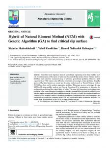
Figure 3 Simulations of GA with SSM by using the one-max problem for: A) the average fitness ( ) and B) the standard deviation ( ) with different values of k the simulations are averaged over 6000 runs A GA with a SSM converges exponentially to the equilibrium point. However, the average fitness ( ) and the variance fitness of population ( 2 ) converge with different characteristic time decays. The characteristic time decay at which 2 (t ) converges to its equilibrium value is 2 log((1 2 pm )2 (1 1 )) . This convergence rate depends on two factors: the convergence due to mutation and the convergence due to selection. The characteristic time decay at which (t ) converges to its equilibrium value is log(1 2 pm ) . The convergence of (t ) is slower; it converges first through the variance and then converges at a rate which is controlled by the mutation rate alone (Amirjanov, 2010). 8
From the equilibrium point an improvement of the average fitness of population is made only by the size adjustment operator, average fitness ( ) and the variance fitness of population ( 2 ) can be calculated as follows (Amirjanov, 2008): (t ) (12) (t ) x(t ) ( x (t ) x(t )) xx 2
x (t ) x(t ) (13) (t ) 2 (t ) x x Analysis of the expressions (10-13) demonstrates that genetic operators of the GA drive the population to the maximum which is amplified by the adjustment operator of a search space. This is achieved as the adjustment operator improves the accuracy of the discrete sampling in the solution space and reduces a computational cost to reach an optimal solution. 2
2.3 Pseudo code of SCRGA The pseudo code of the SCRGA is presented in Figure 4, where the pseudo code of the CRGA is confined by the dotted line. The Input_Data() function establishes the SCRGA parameters and the input data of a multimodal optimization problem. The SCRGA parameters include: the number of optima ( p ), the number of generations ( N gen ),
the number of individuals in the population ( N ind ),
the length of the string ( L ) for binary representation of parameter xi ,
the probability ( Pf ) for Stochastic_Ranking() function,
the probability of crossover ( pc ),
the probability of mutation ( pm ),
the limit ratio of shrinking of the search space size ( s ). Input_Data () for j 1 to p do Initial_Po pulation () for t 1 to N gen do for l 1 to
N ind do
Objective (l ) Penalty (l ) od Stochastic_Ranking() Selection() Crossover() Mutation() Change_Ran ge() CRGA od Add_Constraint() od Report_Data()
Figure 4: Pseudo code of SCRGA 9
The objective function f (x) and the penalty function (x) as per expression (1) are evaluated for all individuals of the population by using Objective() and Penalty() functions, respectively. The Stochastic_Ranking() function ranks the population with the stochastic bubble-sort algorithm. The CRGA implementation uses a binary tournament selection (Selection() function), a single-point crossover of a binary string with probability pc (Crossover() function), a bitwise mutation of a binary string with probability pm (Mutation() function) and the age-based replacement mechanism of surviving individuals (Eiben and Smith, 2003). The Change_Range() function implements a SSM mechanism by shifting a search space to the reference point so that the center of the new search space coincides with the reference point which is the best individual of population; next, the size of a search space is reduced by the coefficient k ( 0 k 1 ), and the lower x(t ) and the upper x(t ) bounds of a new search space are calculated according to the expressions (8, 9).The process of shrinking of a search space size is continued from generation to generation until it has reached its limit which is equal to s of the initial size of the search space. The population evolved for a fixed number of generations ( N gen ) is converged to one of the optima of a multimodal optimization problem. At the end of the convergence, the SCRGA executes the Add_Constraint() function which blocks the niche obtained in the previous run to avoid exploring the same feasible area of a search space. The niche is set as a hypercube around the found optimum according to the expressions (3a, 3b); a new constraint g j (x) is established according to the expression (5) and added to the set of constraints. A similar process of optima searching is continued until all p optima have been obtained. It means that a SCRGA needs p times more iteration time vs. a CRGA. However, a SCRGA, like a sequential niche algorithm can set on the fly a number of optima searched. The Report_Data() function reports data related to the found optima. 3. Computational Results Two groups of test functions were used to verify the performance of proposed algorithm. The first group represents unconstrained multimodal test functions; and the second group contains constrained multimodal test functions. The performance measures consist of a computational cost, a success rate and an accuracy of a SCRGA to find all known optima. The computational cost is defined as a computational time needed to find the complete set of solutions. The time contains the following components: the time for the function evaluations, the time for calculating the penalty functions, and the time for calculating the lower and the upper bounds of the search space. To assess the weight of every time component, a preliminary experiment was designed with unconstrained multimodal test functions represented below. The experiment demonstrated that the function evaluations take significantly longer than any other component. Thus, the computational cost is used as a measure of the number of function evaluations required to find the complete solution set. Success rate is the proportion of runs that find all expected optima. Accuracy is expressed in terms of the root-mean-square (RMS) error in the solutions found. First, the distance between each solution produced by the SCRGA and the nearest exact solution is computed. This distance is then squared, and the RMS value is assessed as the square-root of the mean of these distances. 10
The following common SCRGA parameters were used: L 15 bits , pc 0.9 , pm 0.01 ,
s 0.1 , Pf 0.42 . The probability of crossover pc and the probability of mutation pm are the same as those used by Beasley’s sequential niche genetic algorithm.The length of the binary string ( L ) determines the precision of parameter ( x ) (Eiben and Smith, 2003): xx 2L 1 The precision of the binary representation can be extended by increasing the number of bits L , which considerably slows down the GA (Eiben and Smith, 2003), or by the reduction of the size of the search space ( x x ). By reducing the size of the search space the SCRGA, by the end of any particular run, improves its precision by 10 times. In comparison, the precision of Beasley’s sequential niche genetic algorithm with L 30 is 5 times less than the precision of the SCRGA with L 15 . The reduction of the number of bits L significantly reduces the computational time since less time is needed to execute all operators of a GA and less time is needed for mapping of x parameters from genotype to phenotype spaces. x
For each of the benchmark problems reported, 100 independent runs were executed. 3.1 Unconstrained test functions The proposed algorithm was compared to Beasley’s sequential niche genetic algorithm (BSNGA) by testing the same collection of unconstrained test functions used in the paper (Beasley et al., 1993). BSNGA used the same criteria for an assessment of performance: the number of function evaluations, the success rate and the accuracy of the solutions found. The mathematical formulations of the test functions are given in Table 1. Table 1: Unconstrained test functions Number of maxima ( p )
Range
F1( x) sin6 (5x)
5
x 0,1
2 x 0.1 F 2( x) exp 2 log2 sin 6 5x 0.8
5
x 0,1
Uneven maxima Uneven decreasing maxima
F 3( x) sin6 5 x3 4 0.05
5
x 0,1
5
x 0,1
Himmelblau
F 5( x, y) 200 ( x 2 y 11)2 ( x y 2 7) 2
4
x 6, 6 y 6, 6
No
Type
F1
Equal maxima
F2
Decreasing maxima
F3 F4 F5
Function
2 x 0.08 F 2( x) exp 2 log2 sin 6 5 x3 4 0.05 0.854
The function F1, depicted in Figure 5A, has 5 equally spaced maxima of equal height of 1.0 at x values of 0.1, 0.3, 0.5, 0.7 and 0.9. The function F2, depicted in Figure 5B, is like F1, but the maxima decrease in height exponentially from 1.0 to 0.25. The function F3, depicted in Figure 5C, has 5 equal maxima with a height of 1.0, but the maxima are unevenly spaced at x values of approximately 0.08, 0.246, 0.45, 0.681 and 0.934.
11
Figure 5 Unconstrained test functions: A) F1, B) F2, C) F3, D) F4, and E) F5. The function F4, depicted in Fig. 5D, has 5 maxima with the same height as F2 at the same x values as F3. The function F5, depicted in Fig. 5E, has 4 maxima of equal height of 200 at approximately of x and y values (3.58, -1.86), (3.0, 2.0), (-2.815, 3.125) and (-3.78, -3.28). For the unconstrained test functions the population size of 100 was used, and this value was scaled down according to the number of maxima in the functions. For the functions F1 to F4, the population size ( N ind ) was 20, and for the function F5, Nind 26 . The population size for the functions F1 to F5 is the same that was used by the BSNGA. The fixed number of generations for the functions F1 to F4 was used ( N gen 15 ) as a termination condition of the runs. For the function F5, the SCRGA was terminated after N gen 30 generations. The function F5 is a 2-dimensional function with the inherent complexity (the number of function evaluations) O(n) . It is based on the principle that a GA makes an optimization of n dimensional problem as an optimization of n independent 1-dimensional tasks (Salomon, 1996). Table 2: The experimental parameters of SCRGA Function Parameters F1 F2 F3 F4 F5 N ind 20 20 20 20 26 N gen 15 15 15 15 30
k
0.86
0.86
0.86
0.86
0.93
F6 76
F7 150
F8 20
90 0.97
90 0.97
30 0.93
12
Figure 5: Unconstrained test functions: A) F1, B) F2, C) F3, D) F4, and E) F5 By using the number of generations and the expression (7), the coefficient of shrinking of the search space size k can be calculated as follows: k N gen s
(14)
Consequently, for the functions F1 to F4 k 0.86 , and for the function F5 k 0.93 . The niche sizes around the maxima for the functions F1 to F5 were determined using the expressions (3a, 3b). The SCRGA parameters for the functions F1 to F5 are summarized in Table 2. The experimental results are shown in Table 3, which also represents the results for the BSNGA (Beasley et al., 1993). The comparison of the results indicates that the proposed algorithm (SCRGA) outperformed BSNGA in all terms: a success rate, a computational cost and accuracy. The SCRGA has a success rate of 100%, this means that all the maxima were found in all the runs. The SCRGA needs significantly lesser number of function evaluations to converge to the optima as proved with hypothesis testing by using t test statistic. For all test functions, t t 2 , where t 2 1.97 with level of significance 2 0.025 . For the functions F2 and F4 the computational cost of the BSNGA is double in comparison to the SCRGA. The reduction of the computational cost is an important advantage of SCRGA, particularly in numerical multimodal optimization problems. The SCRGA has a better accuracy than BSNGA for all test functions. Table 3 represents the accuracy of the SCRGA as the mean with the standard error of the mean. The accuracy for the function F5 is somehow lesser in comparison with the functions F1 to F4, because the function F5 has a significantly larger search space than functions F1 to F4.
13
Table 3: Comparisons of the experimental results of the unconstrained test functions Function F1 F2 F3 F4 F5
Computational cost (the number of function evaluations) BSNGA SCRGA 1900 1500 3300 1500 1900 1500 3000 1500 5500 3120
Success rate (%) BSNGA 99 90 100 99 76
SCRGA 100 100 100 100 100
Accuracy
t statistic 10.54 25.87 10.04 44.75 10.17
BSNGA 0.0043 0.0075 0.0039 0.0041 0.2000
SCRGA 0.0028±0.0006 0.0048±0.0008 0.0038±0.0004 0.0039±0.0011 0.0100±0.0157
3.2 Constrained test functions Mathematical formulations for the constrained test functions are provided in Table 4. The relative size of the feasible region in the search space is given by the ratio . The functions F6 and F7 were taken from the conventional benchmark of test functions for constrained numerical optimization (Koziel and Michalewicz, 1999), where the function F7 has an equality constraint. It is common practice to replace the equality constraints h j (x) 0 by a set of inequalities h j (x) and h j (x) for some small 0 (Koziel and Michalewicz, 1999). For this particular case 0.001 was used. The function F8 was taken from (Nguyen, 2008) as a function with static constraints and fixed objective function.The surfaces and the topologies of the search space are depicted in Figure 6 (the function F6), Figure 7 (the function F7) and Figure 8 (the function F8). Table 4: Constrained test functions No
F6
F7
Function
F 6( x, y)
sin 3 (2x) sin(2y)
g1 ( x, y) x 2 y 1
x ( x y)
g 2 ( x, y) 1 x ( y 4) 2
3
g1 ( x, y) y x 2 0.001
F 7( x, y) x 2 ( y 1) 2
F 8(x)
cos
g 2 ( x, y) y x 0.001 2
2
2
F8
Constraint
4
cos
( xi ) 2
i 1
i 1
2
( xi )
i 1
Number of optima ( p)
Range
0.856
4
x 0,10 y 0,10
0.1
2
x 1,1 y 1,1 x1 0,10
2
g1 (x) 0.75
(x i
i 1
2
i xi2
Ratio ( , % )
32.05
2
g 2 ( x)
(x i
2) 12
x2 0,10
2)
i 1
The feasible region of the functions F6 and F7 is less than 1% of the search space. It indicates that a larger population size should be used for sampling of the search space, and more generations are needed to converge to the optimal solution. For the constrained test functions F6 and F7 the population size, 300, was used, which was scaled down according to the number of maxima in the function, that is, for the function F6, Nind 76 and for the function F7, Nind 150 . The number of generations for both functions is equal to 90 ( N gen 90 ). The feasible region of the function F8 is large enough to set the similar values for
14
population size and the number of generations as used in unconstrained test functions. Thus, for the function F8, Nind 20 and N gen 30 were used. The coefficient of shrinking of the search space k is equal to 0.97 for the functions F6 and F7, and k 0.93 for the function F8. These values were calculated by using the number of generations and the expression (14). The SCRGA parameters for the functions F6, F7 and F8 are summarized in Table 2.
Figure 6: Function F6 (a) the surface (b) the topology of the search space
Figure 7: Function F7 (a) the surface (b) the topology of the search space For every subsequent run the SCRGA blocks the niche obtained in the previous run to avoid the exploration of the same feasible area of a search space. The initial feasible area of constrained optimization problem is significantly smaller than a search space, and the expressions (3a, 3b) for setting the niche size should be modified to employ the size of the feasible region instead of the search space size: (15a) xj xj xf r xj xj xf r
(15b)
where x j is the parameter of optimum j {1,, p 1} , p is the number of optima, x j and
xj
are
the
upper
bound
and
the
lower
bounds
of
a
niche
respectively,
15
x f x f 1 x f 1 ,, x fn x fn i {1,, n} defines the hypercube of the feasible region of a search space.
Figure 8: Function F8 (a) the surface (b) the topology of the search space Experimental results are shown in Table 5. The results indicate that the proposed SCRGA algorithm accurately found all maxima for all test functions with high success rate. To find all optima of the problems (F6 and F7) with low ratio ( ) between the sizes of a feasible region and a search space, the SCRGA needs a significant number of function evaluations than for the problems (F8) with high ratio. However, accuracy to obtain all optima depends on the number of the optimal solutions. In Table 5, the SCRGA accuracy of is represented as the mean with the standard error of the mean. Table 5: The experimental results of the constrained test functions Function
Success rate (%)
Computational cost (the number of function evaluations)
Accuracy
F6
100
27360
0.024±0.0014
F7
100
27000
0.044±0.0091
F8
100
7200
0.12±0.0073
The functions F6 and F7 were used as the test functions for an assessment of evolution strategy algorithm (ES) to find a global optimum of constrained numerical optimization problems. It was reported that for the function F6 the standard deviation of objective value of a global maximum ( ) is equal to 2.6e-17 and the computational cost ( c ) is equal to 350000; for the function F7, 8.0e 05 and c 350000 (Runarsson and Yao, 2000). The proposed algorithm obtained the global maximum for the functions F6 and F7 with 5.8e 05 , c 6840 , and 1.2e 03 , c 13500 , respectively. It can be seen that the SCRGA obtained the global maximum for the functions F6 and F7 with high level of precision and at significantly reduced computational cost than ES. It means that the SCRGA which needs significantly lesser computational cost for converging to an optimal solution is a superior evolutionary technique for optimization of continuous multimodal problems where all optima need to be found.
16
4. Conclusions A new evolutionary technique, a sequential changing range genetic algorithm (SCRGA), has been developed for locating all optima of a continuous multimodal problem. The SCRGA involves multiple runs of a changing range genetic algorithm (CRGA), each finding a particular optimum. SCRGA, like any sequential niche technique, avoids researching the area near previously found optima by implementing constraints which convert this area (niche) to an infeasible region. Thus, the SCRGA transforms unconstrained numerical optimization problem to a constrained one. The CRGA was designed with specific features for handling constraints for global numerical optimization problems and it significantly reduced. Computational costs were significantly reduced in finding the optimal solution. The CRGA combines a stochastic ranking of individuals of a population with the shifting and shrinking mechanism which reduces a size of the search space and moves the population to the feasible region. The main advantage of the SCRGA is that it can be used for locating all optima for unconstrained and constrained numerical optimization problems. Several test cases related to unconstrained and constrained numerical optimization problems demonstrated the feasibility of this approach. Computational costs are reduced and the success rate and accuracy of locating all the optima are significantly improved. For locating all optima in constrained numerical optimization problems a new rule was established for setting a niche size around the obtained optimum. This rule is based on the size of the initial feasible region of constrained numerical optimization problems which is smaller than the search space size. In this study, the niche around the located optima is fixed, and is calculated initially by using the size of the initial feasible region. Adaptation of the niche size can be performed for each niche by using the size of the new feasible region which is constructed by implementing new constraints. Changing the niche size for the next search could improve the efficiency of the SCRGA to locate all optima. This approach will be explained later in future work. Test functions in this study consider one and two dimensional cases. The addition of the dimensions would further complicate the problem. It is suggested that the SCRGA will be able to locate all optima for problems with higher dimensions. This is due to the fact that its main component, the CRGA, was successfully used for locating a global optimum in multidimensional numerical constrained optimization problems [15]. However, additional research is needed to prove this assumption.
References Amirjanov, A. (2004) ‘A changing range genetic algorithm’, Int. J. for Numerical Methods in Engineering, Vol. 61, No. 15, pp.2660-2674. Amirjanov, A. (2006) ‘The development a changing range genetic algorithm’, Computer Methods in Applied Mechanics and Engineering, Vol. 195, pp.2495-2508. Amirjanov, A. (2008) ‘Modelling the dynamics of an adjustment of a search space size in a genetic algorithm’, Int. J. Modern Physics C, Vol. 19, No. 7, pp.1047–1062.
17
Amirjanov, A. (2010) ‘The dynamics of a changing range genetic algorithm’, Int. J. for Numerical Methods in Engineering, Vol. 81, pp.892-909. Beasley, D., Bull, D. and Martin, R. (1993) ‘A sequential niche technique for multimodal function optimization’, Evolutionary Computation, Vol. 1, No. 2, pp.101–125. Coello Coello, C.A. (2002) ‘Theoretical and numerical constraint-handling techniques used with evolutionary algorithms: a survey of the state of the art’, Computer Methods in Applied Mechanics and Engineering, Vol. 191, pp.1245–1287. Deb, K. and Goldberg, D. (1989) ‘An investigation of niche and species formation in genetic function optimization’, in Proc. of the Third International Conference on Genetic Algorithms, Morgan Kaufmann, New York, pp.42–55. DeJong, K. (1975) An analysis of the behavior of a class of genetic adaptive systems, Unpublished PhD thesis, University of Michigan. Eiben, A. and Smith, J. (2003) Introduction to evolutionary computing, Springer-Verlag, Berlin. Fiacco, V. and McCormick, G. (1968) Nonlinear Programming: sequential unconstrained minimization techniques, Wiley, New York. Goldberg, D. (1989) ‘Sizing populations for serial and parallel genetic algorithms’, in Proc. of the Third International Conference on Genetic Algorithms, Morgan Kaufmann, New York, pp.70-79. Goldberg, D. and Richardson J. (1987) ‘Genetic algorithms with sharing for multimodal function optimization’, in Proc. of the Second International Conference on Genetic Algorithms, Lawrence Erlbaum, New York, pp.41–49. Hocaoglu, C. and Sanderson, A. (1997) ‘Multimodal function optimization using minimal representation size clustering and its application to planning multipaths’, Evolutionary Computation, Vol. 5, No. 1, pp.81–104. Joines, J. and Houck, C. (1994) ‘On the use of non-stationary penalty functions to solve nonlinear constrained optimization problems with GAs’, in Proc. of the Conference on Evolutionary Computation, IEEE Press, Orlando, pp.579–584. Koziel, S. and Michalewicz, Z. (1999) ‘Evolutionary algorithms, homomorphous mapping, and constrained parameter optimization problems’, Evolutionary Computation, Vol. 7, No. 1, pp.19-44. Kulkarni, K., Moon J., Zhang L., Lucia A. and Linninger A. (2008) ‘Multi-scale modelling and solution multiplicity in catalytic pellet reactors’, Industrial & Engineering Chemistry Research, Vol. 47, pp.8571–8582. Mahfoud, S. (1995) Niching methods for genetic algorithms, Unpublished PhD thesis, University of Illinois at Urbana-Champaign.
18
Mengshoel, O. and Goldberg, D. (2008) ‘The crowding approach to niching in genetic algorithms’, Evolutionary Computation, Vol. 16, No. 3, pp.315–354. Moon, J. and Linninger, A. (2009) ‘A hybrid sequential niche algorithm for optimal engineering design with solution multiplicity’, Computers & Chemical Engineering, Vol. 33, pp.1261-1271. Nguyen, T. (2008) A proposed real-valued dynamic constrained benchmark set, Technical Report, School of Computer Science, University of Birmingham. Petrowski, A. (1996) ‘A clearing procedure as a niching method for genetic algorithms’, in Proc. of the 3rd IEEE International Conference on Evolutionary Computation, IEEE press, pp.798–803. Popp, K. and Schiehlen, W. (2010) Ground vehicle dynamics, Springer-Verlag, Berlin. Runarsson, T. and Yao, X. (2000) ‘Stochastic ranking for constrained evolutionary optimization’, IEEE Transactions on Evolutionary Computation, Vol. 4, No. 3, pp.284-294. Salomon, R. (1996) ‘Reevaluating genetic algorithm performance under coordinate rotation of benchmark functions. A survey of some theoretical and practical aspects of genetic algorithms’, BioSystems, Vol. 39, No. 3, pp.263-278. Siedlecki, W. and Sklansky, J. (1989) ‘Constrained genetic optimization via dynamic rewardpenalty balancing and its use in pattern recognition’, in Proc. of the Third International Conference on Genetic Algorithms, Morgan Kaufmann, New York, pp. 141-149. Tsutsui, S. and Fujimoto, Y. (1997) ‘Forking genetic algorithms: GAs with search space division schemes’, Evolutionary Computation, Vol. 5, No. 1, pp.61-80. Wei, L. and Zhao, M. (2005) ‘A niche hybrid genetic algorithm for global optimization of continuous multimodal functions’, Applied Mathematics and Computation, Vol. 160, pp.649661. Yin, X. and Germay, N. (1993) ‘A fast genetic algorithm with sharing scheme using cluster analysis methods in multi-modal function optimization’, in Proc. of the International Conference on Artificial Neural Nets and Genetic Algorithms, Innsbruck, Austria, pp.450– 457.
19