Chaos and Fractals on the TI Graphing. Calculator. Linda Sundbye, Ph.D.
Department of Mathematical and Computer Sciences. Metropolitan State College
of ...
Chaos and Fractals on the TI Graphing Calculator Linda Sundbye, Ph.D. Department of Mathematical and Computer Sciences Metropolitan State College of Denver Campus Box 38, P.O. Box 173362 Denver, CO 80217
[email protected] A Fractal is a set with ¯ne structure on arbitrarily small scales, with a noninteger dimension, and usually with some degree of self-similarity. Selfsimilar means that the set looks the same on any scale; That is, smaller pieces reproduce the entire set upon magni¯cation. Fractals occur in many natural objects such as coastlines, mountains, canyons, blood vessels, the lungs, and cauli°ower.
1
The Chaos Game
To play this game, we number the vertices of an equilateral triangle 1, 2 and 3. We start with a random initial point in the plane and plot this point. A spinner device is used to randomly pick a number: 1, 2 or 3. From our initial point, we then move half the distance towards that numbered vertex. This point is plotted and becomes our new initial point. We repeat this process a few thousand times. The picture that is generated through this random process is not random at all. The Sierpinski triangle was introduced by Waclaw Sierpinski in 1916.
1
The Sierpinski Triangle
2
Iterated Function Systems and A±ne Transformations
The Sierpinski triangle can also be generated mathematically from the iterated function system (IFS) (see Barnsley) Ã
w1 Ã
w2 Ã
w3 is:
x y x y x y
!
Ã
= !
Ã
= !
Ã
=
:5 0 0 :5 :5 0 0 :5 :5 0 0 :5
!Ã !Ã !Ã
x y x y x y
!
Ã
+ !
Ã
+ !
Ã
+
0 0
!
:25 :50 :50 0
(1) !
(2) !
(3)
The function wi maps the point (x; y) to a new coordinate. The algorithm Randomly pick initial condition (x; y). For K = 1; 3000, randomly pick p 2 [0; 1] If p · 1=3, then map the point (x; y) by w1 If 1=3 < p · 2=3, then map the point (x; y) by w2 If 2=3 < p, then map the point (x; y) by w3 Plot point. Repeat with this point as initial condition.
The mapping w(x; y) is called an a±ne transformation. This type of transformation stretches (or shrinks) and translates. 2
In one dimension, the linear equation w(x) = ax + b is an a±ne transformation. In two dimensions, the mapping µ
x w y
=
µ
a b c d
¶µ
µ
x e + y f
is an a±ne transformation. Codes for several iterated function systems are given below. The quantity p represents the probability of calling the function wi . Thus, for rotationally symmetric fractals, the functions wi have equal probabilities. New fractal images may easily be generated by students by changing the parameter values, probabilities, and by changing the number of equations. (See Barnsley or Scheinerman) IFS w 1 2 3
code a 1/2 1/2 1/2
for b 0 0 0
the c 0 0 0
Sierpinski triangle d e f p 1/2 0 0 1/3 1/2 1/4 1/2 1/3 1/2 1/2 0 1/3
The following pictures were generated on the TI{83 graphing calculator.
3
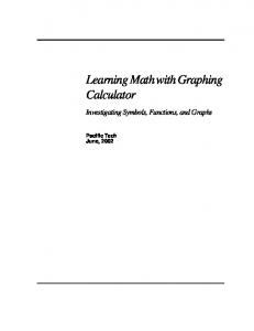
IFS code for the Sierpinski carpet +w a b c d e f +1 1/3 0 0 1/3 0 0 +2 1/3 0 0 1/3 1/3 0 +3 1/3 0 0 1/3 2/3 0 +4 1/3 0 0 1/3 0 1/3 +5 1/3 0 0 1/3 2/3 1/3 +6 1/3 0 0 1/3 0 2/3 +7 1/3 0 0 1/3 1/3 2/3 +8 1/3 0 0 1/3 2/3 2/3
IFS code for the Cantor maze +w a b c d e +1 1/3 0 0 1/3 1/3 +2 0 1/3 1 0 2/3 +3 0 {1/3 1 0 1/3
p 1/8 1/8 1/8 1/8 1/8 1/8 1/8 1/8
f p 2/3 1/7 0 3/7 0 3/7
4
IFS code for +w a +1 0.382 +2 0.382 +3 0.382 +4 0.382 +5 0.382
a 5-sided crystal b c d e 0 0 0.382 0.3072 0 0 0.382 0.6033 0 0 0.382 0.0139 0 0 0.382 0.1253 0 0 0.382 0.4920
IFS code for a +w a b +1 1/3 0 +2 1/3 0 +3 1/3 0 +4 1/3 0 +5 1/3 0
f 0.6190 0.4044 0.4044 0.0595 0.0595
fractal c d e f p 0 1/3 0 0 1/5 0 1/3 2/3 0 1/5 0 1/3 0 2/3 1/5 0 1/3 2/3 2/3 1/5 0 1/3 1/3 1/3 1/5
5
p 1/5 1/5 1/5 1/5 1/5
IFS code for the Koch curve +w a b c d e +1 1/3 0 0 1/3 0 ¡1 1 p +2 1/6 p 1/6 1/3 12 12 1 ¡1 p +3 1/6 p 1/6 1/2 12 12 +4 1/3 0 0 1/3 2/3
IFS code for a fern w a b c d e 1 0 0 0 0.16 0 2 0.85 0.04 {0.04 0.85 0 3 0.2 {0.26 0.23 0.22 0 4 {0.15 0.28 0.26 0.24 0
6
f 0
p 1/4
0
1/4
1 p 12 0
f 0 1.6 1.6 0.44
1/4 1/4
p 0.01 0.85 0.07 0.07
IFS code for a tree +w a b c d e f +1 0 0 0 0.5 0 0 +2 0.42 {0.42 0.42 0.42 0 0.2 +3 0.42 0.42 {0.42 0.42 0 0.2 +4 0.1 0 0 0.1 0 0.2
p 0.05 0.40 0.40 0.15
IFS code for another tree +w a b c d e +1 0.195 {0.488 0.344 0.443 0.4431 +2 0.462 0.414 {0.252 0.361 0.2511 +3 {0.058 {0.070 0.453 {0.111 0.5976 +4 {0.035 0.070 {0.469 {0.022 0.4884 +5 {0.637 0 0 0.501 0.8562
7
f 0.2452 0.5692 0.0969 0.5069 0.2513
p 0.1699 0.1811 0.2161 0.2198 0.2131
3
The Dimension of Self-Similar Fractals
A power law relationship exists between the number of pieces N and the reduction factor r: N=
1 rD
Solving this equation for D gives the similarity dimension: Ds =
ln N ln(1=r)
For the Koch curve, the ¯rst iteration K1 has N = 4 pieces and a reduction factor of r = 1=3. Therefore, Ds = ln 4= ln 3 = 1:26186::::. Similarly, K2 has N = 16 pieces and a reduction factor of r = 1=9 from the original. Therefore, Ds = ln 4= ln 3. Cantor's middle third set has N = 2 pieces and a reduction factor of r = 1=3 at all levels. Therefore, Ds = ln 2= ln 3 = 0:63029::: The Sierpinski triangle has N = 3 pieces and a reduction factor of r = 1=2. And Ds = ln 3= ln 2 = 1:58496:::: The Sierpinski carpet has N = 8 pieces and a reduction factor of r = 1=3. And Ds = ln 8= ln 3 = 1:89279:::: For fractals that are not self-similar, we need yet a di®erent de¯nition of dimension. There are many other de¯nitions of dimension such as the fractal dimension, the Hausdor® dimension and the box dimension, which is a special case of the fractal dimension. (See Barnsley, or Scheinerman)
4
References
[1] Alligood, K. T. Sauer and J. Yorke, Chaos, An Introduction to Dynamical Systems, Springer-Verlag, New York, (1997). [2] Baker, G. and J. Gollub, Chaotic Dynamics, An Introduction, Second Edition, Cambridge University Press, Cambridge, England, (1996). 8
[3] M. Barnsley, Fractals Everywhere, Second Edition, Academic Press, Boston, (1993). [4] J. Gleick, Chaos, Making a New Science, Penguin, New York, (1987). [5] Mandelbrot, B., The Fractal Geometry of Nature, Freeman, San Francisco, (1982). [6] Peitgen, H.O., H. Jurgens, and D. Saupe, Fractals for the Classroom, Part One, Introduction to Fractals and Chaos, Springer Verlag, NCTM, (1992). [7] Peitgen, H.O., H. Jurgens, and D. Saupe, Fractals for the Classroom, Part Two, Complex Systems and Mandelbrot Set, Springer Verlag, NCTM, (1992). [8] Scheinerman, E., Invitation to Dynamical Systems, Prentice Hall, New Jersey, (1996).
9