CHAPTER 1 AUTOMATED DEDUCTION IN REAL GEOMETRY 1

March 27, 2006

12:38

WSPC/Trim Size: 9in x 6in for Review Volume

yang˙xia3

CHAPTER 1 AUTOMATED DEDUCTION IN REAL GEOMETRY

LU YANG 1

Chengdu Institute of Computer Applications Chinese Academy of Sciences, Chengdu 610041, China 2 Guangzhou University, Guangzhou 510405, China E-mail: [email protected] BICAN XIA School of Mathematical Sciences, Peking University Beijing 100871, China E-mail: [email protected] Including three aspects, problem solving, theorem proving and theorem discovering, automated deduction in real geometry essentially depends upon the semi-algebraic system solving. A “semi-algebraic system” is a system consisting of polynomial equations, polynomial inequations and polynomial inequalities, where all the polynomials are of integer coefficients. We give three practical algorithms for the above three kinds of problems, respectively. A package based on the three algorithms for “solving” semi-algebraic systems at each of the three levels has been implemented as Maple programs. The performance of the package on many famous examples are reported.

1. Introduction A semi-algebraic system is a system of polynomial equations, inequalities and inequations. More precisely, we call  p1 (x1 , ..., xn ) = 0, ..., ps (x1 , ..., xn ) = 0,    g1 (x1 , ..., xn ) ≥ 0, ..., gr (x1 , ..., xn ) ≥ 0,  g (x , ..., xn ) > 0, ..., gt (x1 , ..., xn ) > 0,   r+1 1 h1 (x1 , ..., xn ) 6= 0, ..., hm (x1 , ..., xn ) 6= 0, 1

(1)

March 27, 2006

2

12:38


yang˙xia3

L. Yang and B. C. Xia

a semi-algebraic system (sas for short), where n, s ≥ 1, r, t, m ≥ 0 and pi , gj , hk are all polynomials in x1 , ..., xn with integer coefficients. Many problems in both practice and theory can be reduced to problems of solving sas. For example, we may mention some special cases of the “p-3-p” problem15 which originates from computer vision, the problem of constructing limit cycles for plane differential systems26 and the problem of automated discovering and proving for geometric inequalities49,48 . Moreover, many problems in geometry, topology and differential dynamical systems are expected to be solved by translating them into certain semi-algebraic systems. There are two classical methods, Tarski’s method32 and the cylindrical algebraic decomposition (CAD) method proposed by Collins10 , for solving semi-algebraic systems and numerous improvements and progresses11,7,14,3 have been made since then. But this problem is well-known to have for general case double exponential complexity in the number of variables13 . Therefore, the best way to attack quantifier elimination may be that to classify the problems and to offer practical algorithms for some special cases from various applications36,37,38,19,16,48,49,52 . Two classes of sass with strong geometric backgrounds are discussed in this paper. A sas is called a constant-coefficient sas if n = s and {p1 , ..., ps } is assumed to have only a finite number of common zeros while a sas is called a parametric sas if s < n (s indeterminates are viewed as variables and the other n − s indeterminates parameter) and {p1 , ..., ps } is assumed to have only a finite number of common zeros on all the possible values of the parameter. A very recent algorithm to solve general sas (the ideal generated by the polynomials may be of positive dimension) appears in the recent paper by P. Aubry et al.2 . For a constant-coefficient sas, counting and isolating real solutions are two key problems in the study of the real solutions of the system from the viewpoint of symbolic computation. And algorithms for this kind of problems often form the base of some other algorithms for solving parametric sass. T. Becker and V. Weispfenning4 presented an algorithm for isolating the real zeros of a system of polynomial equations by Gröbner bases computing and Sturm theorem. Some effective methods for counting real solutions of a sas are those using trace forms or the rational univariate representation28,29,17 and the algorithm proposed by Xia and Hou44 . Usually, these methods may suggest some algorithms for isolating real solutions of a sas. In Section 2, we present an algorithm45 for isolating the real solutions of a constant-coefficient sas, which, in some sense, can be viewed as a

March 27, 2006

12:38


Automated Deduction in Real Geometry

yang˙xia3

3

generalization of the Uspensky algorithm12 . Lu et al.25 proposed a different algorithm for isolating the real solutions of polynomial equations. Recently, Xia and Zhang46 presented a new and faster algorithm for isolating the real zeros of polynomial equations based on interval arithmetic. Sections 3 and 4 are devoted to algorithms for “solving” parametric sass. Automated theorem proving and discovering on inequalities are always considered as difficult topics in the area of automated reasoning. To prove or disprove a geometric inequality, it is often required to decide whether a parametric sas has any real solutions or not. A so-called “dimension-decreasing” algorithm52,51 is very fast for this kind of problems and is sketched in Section 3. To discover inequality-type theorems automatically, it is often required to find conditions on the parameter of a parametric sas such that the system has a specified number of real solutions. A complete and practical algorithm for this kind of problems is described in Section 4. 2. Find Real Solutions of Geometric Problems In this section we discuss an algorithm for isolating the real solutions of a constant-coefficient sas and its application to finding real solutions of geometric problems. 2.1. Basic Definitions For any polynomial P with positive degree, the leading variable xl of P is the one with greatest index l that effectively appears in P . A triangular set is a set of polynomials {fi (x1 , ..., xi ), fi+1 (x1 , ..., xi+1 ), ..., fl (x1 , ..., xl )} in which the leading variable of fj is xj . If the ideal generated by p1 , ..., pn is zero dimensional, then it is well known that the Ritt-Wu method, Gröbner basis methods or subresultant methods can be used to transform the system of equations into one or more systems in triangular form41,8,34,1,54 . Therefore, in this section, we only consider triangular sets and the problem we discuss is to isolate the real solutions of the following system  f1 (x1 ) = 0,      f 2 (x1 , x2 ) = 0,     · ·  ···· (2) fs (x1 , x2 , ..., xs ) = 0,    g1 (x1 , x2 , ..., xs ) ≥ 0, ..., gr (x1 , x2 , ..., xs ) ≥ 0,     g  r+1 (x1 , x2 , ..., xs ) > 0, ..., gt (x1 , x2 , ..., xs ) > 0,   h1 (x1 , x2 , ..., xs ) 6= 0, ..., hm (x1 , x2 , ..., xs ) 6= 0,

March 27, 2006

12:38


4

yang˙xia3


where s ≥ 1, r, t, m ≥ 0 and {f1 , f2 , ..., fs } is a normal ascending chain54 (also see Definition 1 in this section). We call a system in this form a triangular semi-algebraic system (tsa for short). Given a polynomial g(x), let resultant(g, gx0 , x) be the Sylvester resultant of g and gx0 with respect to x, where gx0 means the derivative of g(x) with respect to x. We call it the discriminant of g with respect to x and denote it by dis(g, x) or simply by dis(g) if its meaning is clear. Given a polynomial g and a triangular set {f1 , f2 , ..., fs }, let rs := g,

rs−i := resultant(rs−i+1 , fs−i+1 , xs−i+1 ),

qs := g,

qs−i := prem(qs−i+1 , fs−i+1 , xs−i+1 ),

i = 1, 2, ..., s; i = 1, 2, ..., s,

where resultant(p, q, x) means the Sylvester resultant of p, q with respect to x and prem(p, q, x) means the pseudo-remainder of p divided by q with respect to x. We denote ri−1 and qi−1 (1 ≤ i ≤ s) by res(g, fs , ..., fi ) and prem(g, fs , ..., fi ) and call them the resultant and pseudo-remainder of g with respect to the triangular set {fi , fi+1 , ..., fs }, respectively. Definition 1: Given a triangular set {f1 , f2 , ..., fs }, denote by Ii (i = 1, ..., s) the leading coefficient of fi in xi . A triangular set {f1 , f2 , ..., fs } is called a normal ascending chain if res(Ii , fi−1 , ..., f1 ) 6= 0 for i = 2, ..., s. Note that I1 6= 0 follows from the definition of a triangular set. Remark 2: A normal ascending chain is also called a regular chain by Kalkbrener21 and a regular set by Wang35 , and was called a proper ascending chain by Yang and Zhang53 . Definition 3: Let a tsa be given as defined in (2), called T . For every fi (i ≥ 1), let CPfi = dis(fi , xi ) (i ≤ 2) and CPfi = res (dis(fi , xi ), fi−1 , fi−2 , ..., f2 ), i > 2. S For any q ∈ {gj | 1 ≤ j ≤ t} {hk | 1 ≤ k ≤ m}, let ½ res (q, fs , fs−1 , ..., f2 ), if s > 1, CPq = q, if s = 1. We define CPT (x1 ) =

Y 1≤i≤s

CPfi ·

Y 1≤j≤t

CPgj ·

Y

CPhk ,

1≤k≤m

and call it the critical polynomial of the system T with respect to x1 . We also denote CPT (x1 ) by CP or CP(x1 ) if its meaning is clear.

March 27, 2006

12:38


yang˙xia3


5

Remark 4: Let a tsa T be given and denote by T1 the system formed by deleting f1 (x1 ) from T . In T1 , we view x1 as a parameter and let it vary continuously on the real number axis. From Theorem 7 below, we know that the number of distinct real solutions of T1 will remain fixed provided that x1 varies on an interval in which there are no real zeros of CPT (x1 ). That is why CPT (x1 ) is called the critical polynomial of the system T . Definition 5: A tsa is regular if resultant(f1 (x1 ), CP(x1 ), x1 ) 6= 0. Remark 6: According to Definition 5, for a regular tsa no CPhk (1 ≤ k ≤ m) has common zeros with f1 (x1 ), which implies that every solution of {f1 = 0, ..., fs = 0} satisfies hk 6= 0 (1 ≤ k ≤ m). Thus if a tsa is regular we can omit the hk ’s in it without loss of generality. Similarly, every solution of {f1 = 0, ..., fs = 0} satisfies gj 6= 0 (1 ≤ j ≤ t). That is to say, each of the inequalities gj ≥ 0 (1 ≤ j ≤ r) in a regular tsa can be treated as gj > 0. 2.2. The Algorithm Given two polynomials p(x), q(x) ∈ Z[x], suppose p(x) and q(x) have no common zeros, i.e., resultant(p, q, x) 6= 0, and α1 < α2 < ... < αn are all distinct real zeros of p(x). By the modified Uspensky algorithm12,30 , we can obtain a sequence of intervals, [a1 , b1 ], ..., [an , bn ], satisfying 1) 2) 3) 4)

αi ∈ [ai , bi ] for i = 1, ..., n, T [ai , bi ] [aj , bj ] = ∅ for i 6= j, ai , bi (1 ≤ i ≤ n) are all rational numbers, and the maximal size of each isolating interval can be less than any positive number given in advance.

Because p(x) and q(x) have no common zeros, the intervals can also satisfy 5) no zeros of q(x) are in any [ai , bi ]. In the following we denote an algorithm to do this by nearzero(p, q, x), or nearzero(p, q, x, ²) if the maximal size of the isolating intervals is specified to be not greater than a positive number ². Theorem 7: Let a regular tsa be given. Suppose f1 (x1 ) has n distinct real zeros; then, by calling nearzero(f1 , CP(x1 ), x1 ) we can obtain a sequence of intervals, [a1 , b1 ], ..., [an , bn ], satisfying, for any [ai , bi ] (1 ≤ i ≤ n) and any β, γ ∈ [ai , bi ],

March 27, 2006

12:38


6

yang˙xia3


1) if s > 1, then the system ½ f2 (β, x2 ) = 0, ..., fs (β, x2 , ..., xs ) = 0, g1 (β, x2 , ..., xs ) > 0, ..., gt (β, x2 , ..., xs ) > 0, and the system ½ f2 (γ, x2 ) = 0, ..., fs (γ, x2 , ..., xs ) = 0, g1 (γ, x2 , ..., xs ) > 0, ..., gt (γ, x2 , ..., xs ) > 0, have the same number of distinct real solutions and, 2) if s = 1, then for any gj (1 ≤ j ≤ t), sign(gj (β)) = sign(gj (γ)), where sign(x) is 1 if x > 0, −1 if x < 0 and 0 if x = 0. Theorem 8: 45 For an irregular tsa T , there is an algorithm which can decompose T into regular systems Ti . Let all the distinct real solutions of a given system be denoted by Rzero(·); then this decomposition satisfies S Rzero(T ) = Rzero(Ti ). By Theorem 8, we only need to consider regular tsas. Given a regular tsa T , for 2 ≤ i ≤ s, 1 ≤ j < i, let  ∂fi ∂fi   , fi , fi−1 , ..., fj+1 ), if 6≡ 0,  res ( ∂xj ∂xj Uij = ∂fi   if ≡ 0,  1, ∂xj MPT (xj ) =

Q j≤k i), when viewed as a function of xi implicitly defined by fj , is monotonic on each isolating interval. The first property is guaranteed by Theorem 7 because the tsa is regular but the second one is not guaranteed. So, in some cases the algorithm does not work. For example, in the case that some zero of f1 (x1 ) is an extreme point of x2 that is viewed as a function of x1 implicitly defined by f2 . We illustrate the algorithm REALZERO in detail by the following simple example which we encountered while solving a geometric constraint problem. Example 10: Given a regular tsa  f1 = 10x2 − 1 = 0,    f2 = −5y 2 + 5xy + 1 = 0, T (1) :  f = 30z 2 − 20(y + x)z + 10xy − 11 = 0,   3 x ≥ 0, y ≥ 0, by REALZERO, we take the following steps to get the isolating intervals. Step 1. MPT (1) (x) = (5x2 + 22)(110x2 + 529) and CPT (1) (x) = x(4 + 5x2 )(7 + 2x2 ) up to some non-zero constants. Because resultant(f1 (x), MPT (1) (x), x) 6= 0, we get S (1) = nearzero(f1 (x), CPT (1) · MPT (1) , x) ·· =

¸ · ¸¸ −3 −5 5 3 , , , . 8 16 16 8

Obviously, the first interval need not to be considered in the following.·So ¸ 5 3 S (1) = , . 16 8 · ¸ 5 3 , . Step 2. S (1) has only one interval I = 16 8 ½ ¾ 5 3 (1) (1) Step 2a. VI = v1 = , v = . 16 2 8

March 27, 2006

12:38


yang˙xia3


9

5 (1) Step 2b. Substituting x = v1 = into T (1) and deleting f1 16 from it, we get  25  2    f2 = 1 + 16 y − 5y = 0, (2) T1 : f = 30z 2 − (20y + 25 )z + 25 y − 11 = 0, 3   4 8   y ≥ 0. 4349 5 Now MPT (2) (y) = −1 and CPT (2) (y) = ( − y + y 2 )y, 1 1 1280 16 by nearzero(f2 (y), CPT (2) · MPT (2) , y), 1 1 ¸ · ¸¸ ·· 5 −3 −5 11 (2) , , , . Obviously, the first inwe get R1 = 8 16 8 16 (2) terval need not to be considered in the following, so, R1 = · ¸ 5 11 3 (1) , . Similarly, by substituting x = v2 = into T (1) , 8 16 8 · ¸ 5 11 (2) we get R2 = , . 8 16 · ¸ 5 11 (2) (2) (2) , and let SI = Step 2c. Merge R1 and R2 into R(2) : 8 16 I × R(2) . Step 3. Because S (1) has only one interval, we have · ¸ · ¸ 5 3 5 11 (2) S (2) = SI = , × , . 16 8 8 16 Now, i = 2 < s = 3, so, repeat Step 2 for S (2) . · ¸ · ¸ 5 3 5 11 Step 2a. S (2) has only one element I = , × , and 16 8 µ 8 16 ½ µ ¶ ¶ 5 5 5 11 (1) (2) (1) (2) VI = (v1 , v1 ) = , , (v2 , v2 ) = , , 16 8 16 16 ¶ ¶¾ µ µ 3 5 3 11 (1) (2) (1) (2) (v3 , v3 ) = , , (v4 , v4 ) = , . 8 8 8 16 5 5 (1) (2) Step 2b. Substituting x = v1 = , y = v1 = into T (1) and 16 8 (3) deleting f1 , f2 from it, we get T1 : {f3 = 640z 2 −400z−193 = 0}. Because this is the last equation in the ascending chain, we let CPT (3) · MPT (3) = 1 and, by nearzero(f3 (z), 1, z), get (3)

1

1

(3)

(3)

(3)

R1 = [[−1, 0], [0, 1]]. Similarly, we have R2 = R3 = R4 = [[−1, 0], [0, 1]].

March 27, 2006

10

12:38


yang˙xia3

L. Yang and B. C. Xia (3)

(3)

(3)

Step 2c. Merge R1 , R2 , R3 (3) and let SI = I × R(3) .

(3)

and R4

into R(3) : [[−1, 0], [0, 1]]

Because S (2) has only one element, we have ·· ¸ · ¸ 5 3 5 11 (3) (3) , × , × [−1, 0], S = SI = 16 8 8 16 ·

¸ · ¸ ¸ 5 3 5 11 , × , × [0, 1] . 16 8 8 16

Now, i = 3 = s, so, go to Step 4 and output ··· ¸ · ¸ ¸ ·· ¸ · ¸ ¸¸ 5 3 5 11 5 3 5 11 , , , , [−1, 0] , , , , , [0, 1] . 16 8 8 16 16 8 8 16 2.3. Realzero and Examples Our method has been implemented as a Maple program realzero in our package. In general, for a sas, the computation of realzero consists of three main steps. First, by the Ritt-Wu method, transform the system of equations into one or more systems in triangular form. In our implementation, we use wsolve33 , a program which realizes Wu’s method under Maple. Second, for each component, check whether it is a regular tsa and, if not, transform it into regular tsas by Theorem 8. Third, apply REALZERO to each resulting regular tsa. There are three basic kinds of calling sequences for a constant-coefficient sas: realzero([p1 , ..., pn ], [q1 , ..., qr ], [g1 , ..., gt ], [h1 , ..., hm ], [x1 , ..., xs ]); realzero([p1 , ..., pn ], [q1 , ..., qr ], [g1 , ..., gt ], [h1 , ..., hm ], [x1 , ..., xs ], width); realzero([p1 , ..., pn ], [q1 , ..., qr ], [g1 , ..., gt ], [h1 , ..., hm ], [x1 , ..., xs ], [w1 , ..., ws ]); .

The command realzero returns a list of isolating intervals for all real solutions of the input system or reports that the method does not work on some components. If the 6th parameter “width”, a positive number, is given, the maximal size of the output intervals is less than or equal to this number. If the 6th parameter is a list of positive numbers, [w1 , ..., ws ], the maximal sizes of the output intervals on x1 , ..., xs are less than or equal to w1 , ..., ws , respectively. If the 6th parameter is omitted, the most convenient width is used for each interval returned. That is to say, the isolating intervals for certain xi are returned provided that they do not intersect with each other. Example 11: This is a problem of solving geometric constraints: Are we

March 27, 2006

12:38


yang˙xia3


11

1 able to construct a triangle with elements a = 1, R = 1 and ha = where 10 a, ha and R denote the side-length, altitude, and circumradius, respectively? A result given by Mitrinovic et al.27 says that there exists a triangle with elements a, R, ha if and only if R1 = 2R − a ≥ 0 and R2 = 8Rha − 4h2a −a2 ≥ 0. From our study49 (also see Section 4 in this paper for details), we know that the result is incorrect. We can also see this from the following 1 computations. For a = 1, R = 1, ha = , we have R1 > 0, R2 < 0 and 10  f1 = 1/100 − 4s(s − 1)(s − b)(s − c) = 0,    f2 = 1/5 − bc = 0,  f3 = 2s − 1 − b − c = 0,   b > 0, c > 0, b + c − 1 > 0, 1 + c − b > 0, 1 + b − c > 0, where s is the half perimeter and b, c are the lengths of the other two sides, respectively. Calling realzero ([f1 , f2 , f3 ], [ ], [b, c, b + c − 1, 1 + c − b, 1 + b − c], [ ], [s, b, c]); we get »»»

»»

– » – » –– »» – » – » –– 259 519 33 17 97 197 259 519 97 99 1 69 , , , , , , , , , , , , 256 512 128 64 128 256 256 512 128 128 4 256

– » – » –– »» – » – » ––– 11 23 73 295 297 595 73 37 21 47 297 595 , , , , , , , , , , , , 256 512 64 128 64 256 256 512 64 32 128 256

which means that there are two different triangles with elements a = 1, R = 1 and ha = 10−1 since b and c are symmetric in the system. The time spent for the computation on a PC (Pentium IV/2.8G) with Maple 8 is 0.2s. Furthermore, say, setting width = 10−6 in the calling sequence: realzero ([f1 , f2 , f3 ], [ ], [b, c, b + c − 1, 1 + c − b, 1 + b − c], [ ], [s, b, c], 10−6 ); we obtain a much more accurate result, »»»

– » – » –– 10624409 1062441 4386135 4386137 64173779 12834761 , , , , , , 10485760 1048576 16777216 16777216 83886080 16777216

»»

– » – » –– 10624409 1062441 3208689 12834761 21930659 1096535 , , , , , , 10485760 1048576 4194304 16777216 83886080 4194304

»»

– » – » –– 152143 12171441 731239 1462479 9623217 24058049 , , , , , , 131072 10485760 4194304 8388608 8388608 20971520

»»

– » – » ––– 152143 12171441 9623217 19246439 2924953 7312403 , , , , , . 131072 10485760 8388608 16777216 16777216 41943040

March 27, 2006

12:38


12

yang˙xia3


The time spent is 0.3s. Example 12: 15 Which triangles can occur as sections of a regular tetrahedron by planes which separate one vertex from the other three? In fact, this is one of the special cases of p-3-p problem which originates from camera calibration. In Section 4, making use of another program called “discoverer”49 , we have got the so-called complete solution classification of this problem. Now, let 1, a, b be the lengths of the three sides of the triangle (assume b ≥ a ≥ 1), and x, y, z the distances from the vertex to the three vertexes of the triangle respectively and suppose that (a, b) is the real roots of {a2 − 1 + b − b2 = 0, 3b6 + 56b4 − 122b3 + 56b2 + 3 = 0}. We want to find x, y and z. Thus, the system is   h1 = x2 + y 2 − xy − 1 = 0,     h2 = y 2 + z 2 − yz − a2 = 0,    h3 = z 2 + x2 − zx − b2 = 0,  h4 = a2 − 1 + b − b2 = 0,     h5 = 3b6 + 56b4 − 122b3 + 56b2 + 3 = 0,    x > 0, y > 0, z > 0, a − 1 ≥ 0, b − a ≥ 0, a + 1 − b > 0. Call realzero ([h1 , h2 , h3 , h4 , h5 ], [b − a, a − 1], [x, y, z, a + 1 − b], [ ], [b, a, x, y, z]); the output is »»»

»

– » – » – » – 73 147 1181 2363 1349206836 348432792 162993 81497 , , , , , , , , 131072 65536 64 128 1024 2048 2188300897 556866289

3247431090114025 202944373270641 , 2465566125550592 154042321050112

––– .

The time spent is 15.02s. Setting width = 10−6 in the calling sequence: realzero ([h1 , h2 , h3 , h4 , h5 ], [b−a, a−1], [x, y, z, a+1−b], [ ], [b, a, x, y, z], 10−6 ); we obtain a much more accurate result, »»»

»

»

– » – » – 162993137 1303945097 1225595355 1225595357 77410187 154820375 , , , , , , 131072000 1048576000 1073741824 1073741824 67108864 134217728

56074137951995697071921875 1057264334012463994320375 , 90106812134321208501993472 1698941787575418678673408

– ,

352619062363191326364463801220259211 55714054304514192059206774779123 , 267676127050613514331758788608000000 42293011923906715097526960128000

The time spent is 19.95s.

––– .

March 27, 2006

12:38


yang˙xia3


13

3. Prove or Disprove Propositions Let Φ be a semi-algebraic system, Φ0 a polynomial equation, inequation or inequality. Prove or disprove that Φ ⇒ Φ0 . Obviously, the statement is true if and only if system Φ ∧ ¬Φ0 is inconsistent, where ¬Φ0 stands for the negative statement of Φ0 . Automated theorem proving in real algebra and real geometry is always considered a difficult topic in the area of automated reasoning. An universal algorithm (such as methods for real quantifier elimination) would be of very high complexity (double exponential complexity in the number of variables for general case). Fortunately, the problem is easier for so-called constructive geometry. Roughly speaking, that is a class of problems where the geometric elements (points, lines and circles) are constructed step by step with rulers and compasses from the ones previously constructed. An inequality of constructive geometry can be converted to an inequality of polynomial/radicals in independent parameter, with some inequality constraints. Let us see the following example: Given real numbers x, y, z, u1 , u2 , u3 , u4 , u5 , u6 satisfying the following 15 conditions  (xy + yz + xz)2 u21 − x3 (y + z)(xy + xz + 4 yz) = 0,       (xy + yz + xz)2 u22 − y 3 (x + z)(xy + yz + 4 xz) = 0,      (xy + yz + xz)2 u23 − z 3 (x + y)(yz + xz + 4 xy) = 0,    (x + y + z)(u2 − x2 ) − xyz = 0, 4 (3) 2  (x + y + z)(u − y 2 ) − xyz = 0,  5     (x + y + z)(u26 − z 2 ) − xyz = 0,      x > 0, y > 0, z > 0,    u1 > 0, u2 > 0, u3 > 0, u4 > 0, u5 > 0, u6 > 0, prove that u1 + u2 + u3 ≤ u4 + u5 + u6 . Eliminating u1 , . . . , u6 from (3) by solving the 6 equations, we convert the proposition to the following inequality which appeared as a conjecture in Shan31 . Example 13: Show that p p x3 (y + z)(xy + xz + 4 yz) y 3 (x + z)(xy + yz + 4 xz) + + xy + yz + xz p xy + yz + xz z 3 (x + y)(yz + xz + 4 xy) ≤ xy + yz + xz

March 27, 2006

12:38


14

yang˙xia3


r x2 +

xyz + x+y+z

r y2 +

xyz + x+y+z

r z2 +

xyz x+y+z

(4)

where x > 0, y > 0, z > 0. This includes 3 variables but 6 radicals, while (3) includes 9 variables. A dimension-decreasing algorithm introduced by the first author can efficiently treat parametric radicals and maximize reduction of the dimensions. Based on this algorithm, a generic program called “BOTTEMA” was implemented on a PC computer. Thousands algebraic and geometric inequalities including hundreds of open problems have been proved or disproved in this way23 . The total CPU time spent for proving 100 basic inequalities, which include some classical results such as Euler’s Inequality, Finsler-Hadwiger’s Inequality, and Gerretsen’s Inequality, from Bottema et al.’s monograph6 “Geometric Inequalities” on a PC (Pentium IV/2.8G) was less than 3 seconds. It can be seen later that the inequality class, to which our algorithm is applicable, is very inclusive. In this section, we deal with a class of propositions which take the following form (though the algorithm is applicable to a more extensive class): Φ1 ∧ Φ2 ∧ · · · ∧ Φs ⇒ Φ0 ,

(5)

where Φ0 , Φ1 , . . . , Φs are algebraic inequalities (see Definition 14) in x, y, z, . . . etc., the hypothesis Φ1 ∧ Φ2 ∧ · · · ∧ Φs defines either an open set (possibly, disconnected) or an open set with the whole/partial boundary. Example 13 may be written as (x > 0) ∧ (y > 0) ∧ (z > 0) ⇒ (4), where the hypothesis (x > 0) ∧ (y > 0) ∧ (z > 0) defines an open set in the parametric space R3 , so it belongs to the class we described. This class covers most of inequalities in Bottema et al.’s book6 and Mitrinovic et al.’s book “Recent Advances in Geometric Inequalities”27 . 3.1. Basic Definitions Before we sketch the so-called dimension-decreasing algorithm, some definitions should be introduced and illustrated. Definition 14: Assume that l(x, y, z, . . .) and r(x, y, z, . . .) are continuous algebraic functions of x, y, z, . . .. We call l(x, y, z, . . .) ≤ r(x, y, z, . . .) or l(x, y, z, . . .) < r(x, y, z, . . .)

March 27, 2006

12:38


yang˙xia3


15

an algebraic inequality in x, y, z . . ., and l(x, y, z, . . .) = r(x, y, z, . . .) an algebraic equality in x, y, z, . . .. Definition 15: Assume that Φ is an algebraic inequality (or equality) in x, y, z, . . . . L(T ) is called a left polynomial of Φ , provided that • L(T ) is a polynomial in T , its coefficients are polynomials in x, y, z, . . . with rational coefficients; • the left-hand side of Φ is a zero of L(T ). The following item is unnecessary for this definition, but it helps to reduce the computational complexity in the process later. • Amongst all the polynomials satisfying the two items above, L(T ) is what has the lowest degree in T . According to this definition, L(T ) = T if the left-hand side is 0, a zero polynomial. The right polynomial of Φ , namely, R(T ), can be defined analogously. Definition 16: Assume that Φ is an algebraic inequality (or equality) in x, y, . . . etc., L(T ) and R(T ) are the left and right polynomials of Φ , respectively. By P (x, y, . . .) denote the resultant of L(T ) and R(T ) with respect to T , and call it the border polynomial of Φ , and the surface defined by P (x, y, . . .) = 0 the border surface of Φ , respectively. The notions of left and right polynomials are needed in practice for computing the border surface more efficiently. In Example 13, we set f1 f2 f3 f4 f5 f6

= (xy + yz + xz)2 u21 − x3 (y + z)(xy + xz + 4 yz), = (xy + yz + xz)2 u22 − y 3 (x + z)(xy + yz + 4 xz), = (xy + yz + xz)2 u23 − z 3 (x + y)(yz + xz + 4 xy), = (x + y + z)(u24 − x2 ) − xyz, = (x + y + z)(u25 − y 2 ) − xyz, = (x + y + z)(u26 − z 2 ) − xyz,

then the left and right polynomials of (4) can be found by successive resultant computation: resultant(resultant(resultant(u1 + u2 + u3 − T, f1 , u1 ), f2 , u2 ), f3 , u3 ), resultant(resultant(resultant(u4 + u5 + u6 − T, f4 , u4 ), f5 , u5 ), f6 , u6 ).

March 27, 2006

12:38


16

yang˙xia3


Removing the factors which do not involve T , we have L(T ) = (x y + x z + y z)8 T 8 − 4(x4 y 2 + 2 x4 y z + x4 z 2 + 4 x3 y 2 z + 4 x3 y z 2 + x2 y 4 + 4 x2 y 3 z + 4 x2 y z 3 + x2 z 4 + 2 x y 4 z + 4 x y 3 z 2 + 4 x y 2 z 3 + 2 x y z 4 + y 4 z 2 + y 2 z 4 )(x y + x z + y z)6 T 6 + · · · , R(T ) = (x + y + z)4 T 8 − 4(x3 + x2 y + x2 z + x y 2 + 3 x y z + x z 2 + y 3 + y 2 z + y z 2 + z 3 ) (x + y + z)3 T 6 + 2(16 x y z 4 + 14 x y 2 z 3 + 14 x y 3 z 2 + 16 x y 4 z + 14 x2 y z 3 + 14 x2 y 3 z + 14 x3 y z 2 + 14 x3 y 2 z + 16 x4 y z + 3 x6 + 5 x4 y 2 + 5 x4 z 2 + 5 x2 y 4 + 5 x2 z 4 + 5 y 4 z 2 + 5 y 2 z 4 + 21 x2 y 2 z 2 + 3 y 6 + 3 z 6 + 6 x5 y + 6 x5 z + 4 x3 y 3 + 4 x3 z 3 + 6 x y 5 + 6 x z 5 + 6 y 5 z + 4 y 3 z 3 + 6 y z 5 ) (x + y + z)2 T 4 − 4(x + y + z)(x6 − x4 y 2 − x4 z 2 + 2 x3 y 2 z + 2 x3 y z 2 − x2 y 4 + 2 x2 y 3 z + 7 x2 y 2 z 2 + 2 x2 y z 3 − x2 z 4 + 2 x y 3 z 2 + 2 x y 2 z 3 + y 6 − y 4 z 2 − y 2 z 4 + z 6 ) (x3 + 3 x2 y + 3 x2 z + 3 x y 2 + 7 x y z + 3 x z 2 + y 3 + 3 y 2 z + 3 y z 2 + z 3 ) T 2 + (−6 x y 2 z 3 − 6 x y 3 z 2 − 6 x2 y z 3 − 6 x2 y 3 z − 6 x3 y z 2 − 6 x3 y 2 z + x6 − x4 y 2 − x4 z 2 − x2 y 4 − x2 z 4 − y 4 z 2 − y 2 z 4 − 9 x2 y 2 z 2 + y 6 + z 6 + 2 x5 y + 2 x5 z − 4 x3 y 3 − 4 x3 z 3 + 2 x y 5 + 2 x z 5 + 2 y 5 z − 4 y 3 z 3 + 2 y z 5 )2 . The successive resultant computation for L(T ) and R(T ) spent CPU time 0.13s and 0.03s, respectively, on a PC (Pentium IV/2.8G) with Maple 8. And then, It took us 33.05s to obtain the border polynomial of degree 100 with 2691 terms. We may of course reform (4) to the equivalent one by transposition of terms, e.g. p p x3 (y + z)(xy + xz + 4 yz) y 3 (x + z)(xy + yz + 4 xz) + + xy + yz + xz p xy + yz + xz r r z 3 (x + y)(yz + xz + 4 xy) xyz xyz − x2 + − y2 + x+y+z x+y+z r xy + yz + xz xyz ≤ z2 + . (6) x+y+z However, the left polynomial of (6) cannot be found on the same computer (with memory 256 Mb) by a Maple procedure as we did for (4), f:=u1+u2+u3-u4-u5-T; for i to 5 do f:=resultant(f,f.i,u.i) od; this procedure did not terminate in 5 hours.

March 27, 2006

12:38


yang˙xia3


17

One might try to compute the border polynomial directly without employing left and right polynomials, that is, using the procedure f:=u1+u2+u3-u4-u5-u6; for i to 6 do f:=resultant(f,f.i,u.i) od; but the situation is not better. The procedure did not terminate in 5 hours either. Example 17: Given an algebraic inequality in x, y, z, ma + mb + mc ≤ 2 s

(7)

where 1p 2 (x + y)2 + 2 (x + z)2 − (y + z)2 , 2 1p mb = 2 (y + z)2 + 2 (x + y)2 − (x + z)2 , 2 1p mc = 2 (x + z)2 + 2 (y + z)2 − (x + y)2 , 2

ma =

s = x+y+z with x > 0, y > 0, z > 0, compute the left, right and border polynomials. Let f1 = 4 m2a + (y + z)2 − 2 (x + y)2 − 2 (x + z)2 , f2 = 4 m2b + (x + z)2 − 2 (y + z)2 − 2 (x + y)2 , f3 = 4 m2c + (x + y)2 − 2 (x + z)2 − 2 (y + z)2 and do successive resultant computation resultant(resultant(resultant(ma + mb + mc − T, f1 , ma ), f2 , mb ), f3 , mc ), we obtain a left polynomial of (7): T 8 − 6 (x2 + y 2 + z 2 + x y + y z + z x) T 6 + 9(x4 + 2 x y z 2 + y 4 + 2 x z 3 + 2 x3 y + z 4 + 3 y 2 z 2 + 2 y 2 z x + 2 y 3 z + 2 y z 3 + 3 x2 z 2 + 2 x3 z + 2 x2 y z + 2 x y 3 + 3 x2 y 2 )T 4 − (72 x4 y z + 78 x3 y z 2 + 4 x6 + 4 y 6 + 4 z 6 + 12 x y 5 − 3 x4 y 2 − 3 x2 z 4 − 3 x2 y 4 − 3 y 4 z 2 − 3 y 2 z 4 − 3 x4 z 2 − 26 x3 y 3 − 26 x3 z 3 − 26 y 3 z 3 + 12 x z 5 + 12 y 5 z + 12 y z 5 + 12 x5 z + 12 x5 y + 84 x2 y 2 z 2 + 72 x y z 4 + 72 x y 4 z + 78 x y 3 z 2 + 78 x y 2 z 3 + 78 x2 y z 3 + 78 x3 y 2 z + 78 x2 y 3 z)T 2 + 81 x2 y 2 z 2 (x + y + z)2 .

(8)

March 27, 2006

18

12:38


yang˙xia3


It is trivial to find a right polynomial for this inequality because the righthand side contains no radicals. We simply take T − 2 (x + y + z).

(9)

Computing the resultant of (8) and (9) with respect to T , we have (144 x5 y + 144 x5 z + 780 x4 y 2 + 1056 x4 y z + 780 x4 z 2 + 1288 x3 y 3 + 3048 x3 y 2 z + 3048 x3 y z 2 + 1288 x3 z 3 + 780 x2 y 4 + 3048 x2 y 3 z + 5073 x2 y 2 z 2 + 3048 x2 y z 3 + 780 x2 z 4 + 144 x y 5 + 1056 x y 4 z + 3048 x y 3 z 2 + 3048 x y 2 z 3 + 1056 x y z 4 + 144 x z 5 + 144 y 5 z + 780 y 4 z 2 + 1288 y 3 z 3 + 780 y 2 z 4 + 144 y z 5 )(x + y + z)2 . Removing the non-vanishing factor (x+y+z)2 , we obtain the border surface 144 x5 y + 144 x5 z + 780 x4 y 2 + 1056 x4 y z + 780 x4 z 2 + 1288 x3 y 3 + 3048 x3 y 2 z + 3048 x3 y z 2 + 1288 x3 z 3 + 780 x2 y 4 + 3048 x2 y 3 z + 5073 x2 y 2 z 2 + 3048 x2 y z 3 + 780 x2 z 4 + 144 x y 5 + 1056 x y 4 z + 3048 x y 3 z 2 + 3048 x y 2 z 3 + 1056 x y z 4 + 144 x z 5 + 144 y 5 z + 780 y 4 z 2 + 1288 y 3 z 3 + 780 y 2 z 4 + 144 y z 5 = 0.

(10)

3.2. The Dimension-decreasing Algorithm We take the following procedures when the conclusion Φ0 in (5) is of type ≤. (As for Φ0 of type 0, then the proposition is false.

March 27, 2006

20

12:38


yang˙xia3


Otherwise, δ0 < 0 holds over Q because every connected component of Q contains a test point and δ0 keeps the same sign over each component ∆λ , hence δ0 ≤ 0 holds over A by continuity, so it also holds over A ∪ B, i.e., the proposition is true. The above procedures sometimes may be simplified. When the conclusion Φ0 belongs to an inequality class called “class CGR”, what we need to do in step 3 is to compare the greatest roots of left and right polynomials of Φ0 over the test values. Definition 18: An algebraic inequality is said to belong to class CGR if its left-hand side is the greatest (real) root of the left polynomial L(T ), and the right-hand side is that of the right polynomial R(T ). It is obvious in Example 13 that the left- and right-hand sides of the inequality (4) are the greatest roots of L(T ) and R(T ), respectively, because all the radicals have got positive signs. Thus, the inequality belongs to class CGR. What we need to do is to verify whether the greatest root of L(T ) is less than or equal to that of R(T ), that is much easier than determine which is greater between two complicated radicals, in the sense of accurate computation. If an inequality involves only mono-layer radicals, then it always can be transformed into an equivalent one which belongs to class CGR by transposition of terms. Actually, most of the inequalities in Bottema et al.6 and Mitrinovic et al.27 , including most of the examples in this section, belong to the class CGR. For some more material, see Yang47 . 3.3. Inequalities on Triangles An absolute majority of the hundreds inequalities discussed in Bottema et al.6 are on triangles, so are the thousands appeared in various publications since then. For geometric inequalities on a single triangle, usually the geometric invariants are used as global variables instead of Cartesian coordinates. By a, b, c denote the side-lengths, s the half perimeter, i.e. 12 (a+b+c), and x, y, z denote s − a, s − b, s − c, respectively, as people used to do. In additional, by A, B, C the interior angles, S the area, R the circumradius, r the inradius, ra , rb , rc the radii of escribed circles, ha , hb , hc the altitudes, ma , mb , mc the lengths of medians, wa , wb , wc the lengths of interior angular bisectors, and so on.

March 27, 2006

12:38



yang˙xia3

21

People used to choose x, y, z as independent variables and others dependent. Sometimes, another choice is better for decreasing the degrees of polynomials occurred in the process. An algebraic inequality Φ(x , y, z ) can be regarded as a geometric inequality on a triangle if • x > 0, y > 0, z > 0; • the left- and right-hand sides of Φ, namely l(x, y, z) and r(x, y, z), both are homogeneous; • l(x, y, z) and r(x, y, z) have the same degree. The item 1 means that the sum of two edges of a triangle is greater than the third edge. The items 2 and 3 means that a similar transformation does not change the truth of the proposition. For example, (7) is such an inequality for its left- and right-hand sides, ma + mb + mc and 2 s, both are homogeneous functions (of x, y, z) with degree 1. In addition, assume that the left- and right-hand sides of Φ(x , y, z ), namely, l(x, y, z) and r(x, y, z), both are symmetric functions of x, y, z. It does not change the truth of the proposition to replace x, y, z in l(x, y, z) and r(x, y, z) with x0 , y 0 , z 0 where x0 = ρ x, y 0 = ρ y, z 0 = ρ z and ρ > 0. Clearly, the left and right polynomials of Φ(x 0 , y 0 , z 0 ), namely, L(T, x0 , y 0 , z 0 ) and R(T, x0 , y 0 , z 0 ), both are symmetric with respect to x0 , y 0 , z 0 , so they can be re-coded in the elementary symmetric functions of x0 , y 0 , z 0 , say, Hl (T, σ1 , σ2 , σ3 ) = L(T, x0 , y 0 , z 0 ),

Hr (T, σ1 , σ2 , σ3 ) = R(T, x0 , y 0 , z 0 ),

where σ1 = x0 + y 0 + z 0 , σ2 = x0 y 0 + y 0 z 0 + z 0 x0 , σ3 = x0 y 0 z 0 . q x+y+z 0 0 0 0 0 0 Setting ρ = x y z , we have x y z = x + y + z , i.e., σ3 = σ1 . Further, letting s = σ1 (= σ3 ),

p = σ2 − 9,

we can transform L(T, x0 , y 0 , z 0 ) and R(T, x0 , y 0 , z 0 ) into polynomials in T, p, s, say, F (T, p, s) and G(T, p, s). Especially if F and G both have only even-degree terms in s, then they can be transformed into polynomials in T, p and q where q = s2 − 4 p − 27. Usually the degrees and the numbers of terms of the latter are much less than those of L(T, x, y, z) and R(T, x, y, z). We thus construct the border surface which is encoded in p, s or p, q, and do the decomposition described in last section on (p, s)-plane or (p, q)-plane instead of R3 . This may reduce the computational complexity considerably

March 27, 2006

12:38


22

yang˙xia3


for a large class of geometric inequalities. The following example is also taken from Bottema et al.6 . Example 19: By wa , wb , wc and s denote the interior angular bisectors and half the perimeter of a triangle, respectively. Prove wb wc + wc wa + wa wb ≤ s2 . It is well-known that p x (x + y)(x + z)(x + y + z) wa = 2 , 2x + y + z p y (x + y)(y + z)(x + y + z) wb = 2 , 2y + x + z p z (x + z)(y + z)(x + y + z) , wc = 2 2z + x + y and s = x + y + z. By successive resultant computation as above, we get a left polynomial which is of degree 20 and has 557 terms, while the right polynomial T − (x + y + z)2 is very simple, and the border polynomial P (x, y, z) is of degree 15 and has 136 terms. However, if we encode the left and right polynomials in p, q, we get (9 p + 2 q + 64)4 T 4 − 32 (4 p + q + 27) (p + 8) (4 p2 + p q + 69 p + 10 q + 288) (9 p + 2 q + 64)2 T 2 − 512 (4 p + q + 27)2 (p + 8)2 (9 p + 2 q + 64)2 T + 256(4 p + q + 27)3 (p + 8)2 (−1024 − 64 p + 39 p2 − 128 q − 12 p q − 4 q 2 + 4 p3 + p2 q) and T − 4 p − q − 27, respectively, hence the border polynomial Q(p, q) = 5600256 p2 q + 50331648 p + 33554432 q + 5532160 p3 + 27246592 p2 + 3604480 q 2 + 22872064 p q + 499291 p4 + 16900 p5 + 2480 q 4 + 16 q 5 + 143360 q 3 + 1628160 p q 2 + 22945 p4 q + 591704 p3 q + 11944 p3 q 2 + 2968 p2 q 3 + 242568 p2 q 2 + 41312 p q 3 + 352 p q 4 which is of degree 5 and has 20 terms only. The whole proving process in this way spend about 0.03s on the same machine.

March 27, 2006

12:38



yang˙xia3

23

3.4. BOTTEMA and Examples As a prover, the whole program is written in Maple including the cell decomposition, without external packages employed. On verifying an inequality with BOTTEMA, we only need to type in a proving command, then the machine will do everything else. If the statement is true, the computer screen will show “The inequality holds”; otherwise, it will show “The inequality does not hold ” with a counter-example. There are three kinds of proving commands: prove, xprove and yprove.

prove – prove a geometric inequality on a triangle, or an equivalent algebraic inequality. Calling Sequence: prove(ineq); prove(ineq, ineqs); Parameters: ineq – an inequality to be proven, which is encoded in the geometric invariants listed later. ineqs – a list of inequalities as the hypothesis, which is encoded as well in the geometric invariants listed later. Examples: > read bottema; > prove(a^2+b^2+c^2>=4*sqrt(3)*S+(b-c)^2+(c-a)^2+(a-b)^2); The theorem holds > prove(cos(A)>=cos(B),[a read bottema; > xprove(sqrt(u^2+v^2)+sqrt((1-u)^2+(1-v)^2)>=sqrt(2), [u xprove(f>=42496/10000,[y>1]); The theorem holds > xprove(f>=42497/10000,[y>1]); with a counter example ·

¸ 29 294117648 ,y= 32 294117647 The theorem does not hold x=

yprove – prove an algebraic inequality in general. Calling Sequence: yprove(ineq); yprove(ineq, ineqs); Parameters: ineq – an algebraic inequality to be proven. ineqs – a list of algebraic inequalities as the hypothesis. Examples: > read bottema; > f:=x^6*y^6+6*x^6*y^5-6*x^5*y^6+15*x^6*y^4-36*x^5*y^5+15*x^4*y^6 +20*x^6*y^3-90*x^5*y^4+90*x^4*y^5-20*x^3*y^6+15*x^6*y^2 -120*x^5*y^3+225*x^4*y^4-120*x^3*y^5+15*x^2*y^6+6*x^6*y -90*x^5*y^2+300*x^4*y^3-300*x^3*y^4+90*x^2*y^5-6*x*y^6+x^6 -36*x^5*y+225*x^4*y^2-400*x^3*y^3+225*x^2*y^4-36*x*y^5+y^6 -6*x^5+90*x^4*y-300*x^3*y^2+300*x^2*y^3-90*x*y^4+6*y^5+15*x^4 -120*x^3*y+225*x^2*y^2-120*x*y^3+15*y^4-20*x^3+90*x^2*y -90*x*y^2+20*y^3+16*x^2-36*x*y+16*y^2-6*x+6*y+1: > yprove(f>=0); The theorem holds

March 27, 2006

12:38



yang˙xia3

25

3.5. More Examples All the examples in this subsection are computed by BOTTEMA on a PC (Pentium IV/2.8G) with Maple 8. The following example is the well-known Janous’ inequality20 which was proposed as an open problem in 1986 and solved in 1988. Example 20: Denote the three medians and perimeter of a triangle by ma , mb , mc and 2 s , show that 1 1 1 5 + + ≥ . ma mb mc s The left-hand side of the inequality implicitly contains three radicals. BOTTEMA automatically interprets the geometric proposition to algebraic

one before proves it. The total CPU time spent for this example is 3.58s. The next example was proposed as an open problem, E. 3146∗ , in the Amer. Math. Monthly 93:(1986), 299. Example 21: Denote the side-lengths and half perimeter of a triangle by a, b, c and s, respectively. Prove or disprove p p p √ √ √ 2 s( s − a + s − b + s − c) ≤ 3 ( bc(s − a) + ca(s − b) + ab(s − c)). The proof took us 9.91s on the same machine. The following open problem appeared as Problem 169 in Mathematical Communications (in Chinese). Example 22: Denote the radii of the escribed circles and the interior angle bisectors of a triangle by ra , rb , rc and wa , wb , wc , respectively. Prove or disprove √ 3

1 (wa + wb + wc ). 3 In other words, the geometric average of ra , rb , rc is less than or equal to the arithmetic average of wa , wb , wc . ra r b r c ≤

The right-hand side of the inequality implicitly contains 3 radicals. BOTTEMA proved this conjecture with CPU time 96.60s. One more conjecture proposed by J. Liu31 was proven on the same machine with CPU time 52.36s. That is: Example 23: Denote the side lengths, medians and interior-anglebisectors of a triangle by a, b, c, ma , mb , mc and wa , wb , wc , respectively.

March 27, 2006

12:38


26

yang˙xia3


Prove or disprove 2 a ma + b mb + c mc ≤ √ (wa2 + wb2 + wc2 ). 3 The following conjecture was first proposed by J. Garfunkel at Crux Math. in 1985, then re-proposed twice again by Mitrinovic et al.27 and Kuang22 . Example 24: Denote the three angles of a triangle by A, B, C. Prove or disprove B−C C −A A−B + cos + cos ≤ 2 2 2 1 A B C √ (cos + cos + cos + sin A + sin B + sin C ). 2 2 2 3

cos

It was proven with CPU time 21.75s. A. Oppenheim studied the following inequality27 in order to answer a problem proposed by P. Erdös. Example 25: Let a, b, c and ma , mb , mc be the side lengths and medians of a triangle, respectively. If c = min{a, b, c}, then √ 2 ma + 2 mb + 2 mc ≤ 2 a + 2 b + (3 3 − 4) c. The hypothesis includes one more condition, c = min{a, b, c}, so we type in prove(2*ma+2*mb+2*mc 0, ..., gt (U, x1 , ..., xs ) > 0,    h1 (U, x1 , ..., xs ) 6= 0, ..., hm (U, x1 , ..., xs ) 6= 0,

(13)

where U = (xs+1 , ..., xn ) are viewed as parameter and are usually denoted by U = (u1 , ..., ud ). We call a system in this form a parametric tsa. All the definitions for a tsa are valid for a parametric tsa. Definition 30: Given a parametric tsa T , let BPf1 = CPf1 and BPq = resultant(CPq , f1 , x1 ), q ∈ {fi , gj , hk |1 < i ≤ s, 1 ≤ j ≤ t, 1 ≤ k ≤ m}. Q Q Q We define BPT (U ) = 1≤i≤s BPfi · 1≤j≤t BPgj · 1≤k≤m BPhk and call it the boundary polynomial of T . It is also denoted by BP. Then, a regular parametric tsa can be defined by BP 6= 0. As remarked in Section 2, if a parametric tsa is regular we can omit the hk ’s in it without loss of generality and each of the inequalities gj ≥ 0 (1 ≤ j ≤ r) in the system can be treated as gj > 0. Definition 31: Given a polynomial with real symbolic coefficients, f (x) = a0 xn + a1 xn−1 + ... + an , the following 2n × 2n matrix in terms of the

March 27, 2006

12:38


30

yang˙xia3


coefficients, 

a0 0           

a1 a2 na0 (n − 1)a1 a0 a1 0 na0

··· ··· ··· ··· ··· ··· a0 0

 an  an−1   an−1 an   2an−2 an−1    ···   ···  a1 a2 · · · an  na0 (n − 1)a1 · · · an−1

is called the discrimination matrix of f (x), and denoted by Discr (f ). Denote by dk the determinant of the submatrix of Discr (f ), formed by the first k rows and the first k columns for k = 1, 2, ..., 2n. Definition 32: Let D0 = 1 and Dk = d2k , k = 1, ..., n. We call the (n+1)tuple [D0 , D1 , D2 , ..., Dn ] the discriminant sequence of f (x), and denote it by DiscrList (f ). Obviously, the last term Dn is dis(f, x). Definition 33: We call the list [sign(A0 ), sign(A1 ), sign(A2 ), · · · , sign(An )] the sign list of a given sequence Definition 34: Given a sign list [s1 , s2 , · · · , sn ], we construct a new list [t1 , t2 , · · · , tn ] as follows: (which is called the revised sign list) • If [si , si+1 , · · · , si+j ] is a section of the given list, where si 6= 0, si+1 = · · · = si+j−1 = 0, si+j 6= 0, then, we replace the subsection [si+1 , · · · , si+j−1 ] by the first j − 1 terms of [−si , −si , si , si , −si , −si , si , si , · · · ], that is, let ti+r = (−1)[(r+1)/2] · si ,

r = 1, 2, · · · , j − 1.

• Otherwise, let tk = sk , i.e. no changes for other terms.

March 27, 2006

12:38



yang˙xia3

31

Theorem 35: Given a polynomial f (x) with real coefficients, f (x) = a0 xn + a1 xn−1 + · · · + an , if the number of sign changes of the revised sign list of [D0 , D1 (f ), D2 (f ), · · · , Dn (f )] is ν, then the number of distinct pairs of conjugate imaginary roots of f (x) equals ν. Furthermore, if the number of non-vanishing members of the revised sign list is l, then the number of distinct real roots of f (x) equals l − 1 − 2ν. Definition 36: Given two polynomials g(x) and f (x) = a0 xn + a1 xn−1 + · · · + an , let r(x) = rem(f 0 g, f, x) = b0 xn−1 + b1 xn−2 + · · · + bn−1 . The following 2n × 2n matrix  a0 a1 a2 · · ·  0 b 0 b1 · · ·   a a ··· 0 1   0 b0 · · ·    ···   ···   a0 0



an bn−1 an−1 bn−2 ··· ··· a1 b0

an bn−1

a2 · · · an b1 · · · bn−1

           

is called the generalized discrimination matrix of f (x) with respect to g(x), and denoted by Discr (f, g). Definition 37: Given two polynomials f (x) and g(x). Let D0 = 1 and denote by D1 (f, g), D2 (f, g), · · · , Dn (f, g) the even order principal minors of Discr (f, g). We call [D0 , D1 (f, g), D2 (f, g), · · · , Dn (f, g)] the generalized discriminant sequence of f (x) with respect to g(x), and denote it by GDL(f, g). Clearly, GDL(f, 1) = DiscrList (f ).

March 27, 2006

12:38

32


yang˙xia3


Theorem 38: Given two polynomials f (x) and g(x), if the number of sign changes of the revised sign list of GDL(f, g) is ν, and the number of non-vanishing members of the revised sign list is l, then l − 1 − 2ν = c(f, g+ ) − c(f, g− ), where c(f, g+ ) = card({x ∈ R|f (x) = 0, g(x) > 0}), c(f, g− ) = card({x ∈ R|f (x) = 0, g(x) < 0}). Definition 39: A normal ascending chain {f1 , ..., fs } is simplicial with respect to a polynomial g if either prem(g, fs , ..., f1 ) = 0 or res(g, fs , ..., f1 ) 6= 0. Theorem 40: 54 For a triangular set AS : {f1 , ..., fs } and a polynomial g, there is an algorithm which can decompose AS into some normal ascending chains ASi : {fi1 , fi2 , ..., fis } (1 ≤ i ≤ n), such that every chain is simplicial with respect to g and this decomposition satisfies that S Zero(AS) = 1≤i≤n Zero(ASi ), where Zero(·) means the set of zeros of a given system. Remark 41: We call this decomposition the rsd decomposition of AS with respect to g and the algorithm is called the rsd algorithm. The decomposition and the algorithm were called wr decomposition and wr algorithm respectively by Yang, Zhang and Hou54 . Wang35 proposed a similar decomposition algorithm. By Theorem 40, we always consider the triangular set {f1 , f2 , ..., fs } that appears in a tsa as a normal ascending chain, without loss of generality. Definition 42: 24 Let Dkt be the submatrix of Discr (f ), formed by the first 2n − 2k rows, the first 2n − 2k − 1 columns and the (2n − 2k + t)th column, where 0 ≤ k ≤ n − 1, 0 ≤ t ≤ 2k. Let |Dkt | = det(Dkt ). We call |Dk0 | (0 ≤ k ≤ n − 1) the kth principal subresultant of f (x). Obviously, |Dk0 | = Dn−k (0 ≤ k ≤ n − 1). Definition 43: 24 Let Qn+1 (f, x) = f (x), Qn (f, x) = f 0 (x), and for k = Pk 0, 1, ..., n−1, Qk (f, x) = t=0 |Dkt |xk−t = |Dk0 |xk +|Dk1 |xk−1 +...+|Dkk |. We call {Q0 (f, x), ..., Qn+1 (f, x)} the subresultant polynomial chain of f (x). Theorem 44: 55 Suppose {f1 , f2 , ..., fj } is a normal ascending chain, where K is a field and fi ∈ K[x1 , ..., xi ], (i = 1, 2, ..., j) and f (x) =

March 27, 2006

12:38



yang˙xia3

33

a0 xn + a1 xn−1 + ... + an−1 x + an is a polynomial in K[x1 , ..., xi ][x], let P Dk = prem(|Dk0 |, fj , ..., f1 ) = prem(Dn−k , fj , ..., f1 ), (0 ≤ k < n). If for some k0 ≥ 0, res(a0 , fj , ..., f1 ) 6= 0 and P D0 = · · · = P Dk0 −1 = 0, res(|Dk00 |, fj , ..., f1 ) 6= 0, then, we have gcd(f, fx0 ) = Qk0 (f, x) in K[x1 , ..., xj ]/(f1 , ..., fj ). Theorem 45: For an irregular parametric tsa T , there is an algorithm which can decompose T into regular systems Ti . Let all the distinct real solutions of a given system be denoted by Rzero(·); then this decomposition S satisfies Rzero(T ) = Rzero(Ti ). Proof: For T , BP= resultant(f1 , CP, x1 ) = 0. • If there is some CPhk such that resultant(f1 , CPhk , x1 ) = 0, do the rsd decomposition of {f1 , ..., fs } with respect to hk and, without loss of generality, suppose we get two new chains {A1 , ..., As } and {B1 , ..., Bs }, in which prem(hk , As , ..., A1 ) = 0 but res(hk , Bs ..., B1 ) 6= 0. If we replace {f1 , ..., fs } by {B1 , ..., Bs } in T , the new system is regular and has the same real solutions as those of the original system. Obviously, another system obtained by replacing {f1 , ..., fs } with {A1 , ..., As } in T , has no real solutions. • If there is some CPgj such that resultant(f1 , CPgj , x1 ) = 0, do the rsd decomposition of {f1 , ..., fs } with respect to gj and suppose we get {A1 , ..., As } and {B1 , ..., Bs }, in which prem(gj , As , ..., A1 ) = 0 but res(gj , Bs ..., B1 ) 6= 0. Now, if gj > 0 in T , we simply replace {f1 , ..., fs } by {B1 , ..., Bs }. The new system is regular and has the same real solutions as those of the original system. If gj ≥ 0 in T , we first get a new system T1 by replacing {f1 , ..., fs } with {B1 , ..., Bs } and then, get another new system T2 by replacing {f1 , ..., fs } with {A1 , ..., As } and deleting gj from it. These two systems are both S regular and we have Rzero(T ) = Rzero(T1 ) Rzero(T2 ). • If there is some CPfi such that resultant(f1 , CPfi , x1 ) = 0, let [D1 , ..., Dni ] be the discriminant sequence of fi with respect to xi . First of all, we do the rsd decomposition of {f1 , ..., fi−1 } with respect to Dni and suppose we get {A1 , ..., Ai−1 } and {B1 , ..., Bi−1 }, in which prem(fi , Ai−1 , ..., A1 ) = 0 but res(fi , Bi−1 ..., B1 ) 6= 0. Step 1, replacing {f1 , ..., fi−1 } with {B1 , ..., Bi−1 }, we will get a regular system. Step 2, let us consider the system obtained by replacing {f1 , ..., fi−1 } with {A1 , ..., Ai−1 } which is still irregular. Consider Dni −1 , the next term in [D1 , ..., Dni ].

March 27, 2006

12:38


34

yang˙xia3


If res(Dni −1 , Ai−1 , ..., A1 ) = 0, do the rsd decomposition of {A1 , ..., Ai−1 } with respect to Dni −1 . Keep repeating the same procedure until at a certain step we have, for certain Di0 and {A¯1 , ..., A¯i−1 }, res(Di0 , A¯i−1 , ..., A¯1 ) 6= 0 and ∀j (i0 < j ≤ ni ), prem(Dj , A¯i−1 , ..., A¯1 ) = 0. Note that this procedure must terminate because {f1 , ..., fs } being a normal ascending chain implies res(Ii , fi−1 , ..., f1 ) 6= 0 and D1 = ni Ii2 implies res(D1 , fi−1 , ..., f1 ) 6= 0. By Theorem 2.3, gcd(fi , fi0 ) = Qni −i0 (fi , xi ) in K[x1 , ..., xi−1 ]/(A¯1 , ..., A¯i−1 ). Now, let f¯i be the pseudo-quotient of fi divided by gcd(fi , fi0 ) and replace {f1 , ..., fi−1 , fi } with {A¯1 , ..., A¯i−1 , f¯i }, the new system will be regular. If the new regular systems are Tj (1 ≤ j ≤ ji ), it is easy to S see that Rzero(T ) = 1≤j≤ji Rzero(Tj ). By Theorem 45, every parametric tsa in the rest of this section can be treated as a regular one. 4.2. The Algorithm Let ps = {pi |1 ≤ j ≤ n} be a nonempty, finite set of polynomials. We define mset(ps) = {1} ∪ {pi1 pi2 · · · pik |1 ≤ k ≤ n, 1 ≤ i1 < i2 < · · · < ik ≤ n}. Given a parametric tsa T , we define Ps+1 = {g1 , g2 , · · · , gt }; [ Ui = GDL(fi , q), q∈mset(Pi+1 )

Pi = {h(u, x1 , · · · , xi−1 )|h ∈ Ui },

for i = s, s − 1, · · · , 2;

P1 (g1 , g2 , · · · , gt ) = {h(u)|h ∈ U1 }, where Ui means the set consisting of all the polynomials in each GDL(fi , q) where q belongs to mset(Pi+1 ). Analogously, we can define P1 (g1 , · · · , gj ) (1 ≤ j ≤ t). It is clear that all the factors of the boundary polynomial, BP, of T are included in P1 (g1 , g2 , · · · , gt ). With a little abuse of notations, we write BP ⊆ P1 (g1 , g2 , · · · , gt ). Theorem 46: The necessary and sufficient condition for a parametric tsa T to have a given number of distinct real solution(s) can be expressed in terms of the signs of the polynomials in P1 (g1 , g2 , · · · , gt ).

March 27, 2006

12:38



yang˙xia3

35

Proof: First of all, we regard fs and every gi as polynomials in xs . By Theorems 35 and 38 we know that under constraints {gi ≥ 0|1 ≤ i ≤ t}, the number of distinct real solutions of fs = 0 can be determined by the signs of polynomials in Ps . Let hj (1 ≤ j ≤ l) be the polynomials in Ps , then we regard every hj and fs−1 as polynomials in xs−1 . Repeating the same argument as that for fs and gi ’s, we get that, under constraints {gi ≥ 0|1 ≤ i ≤ t}, the number of distinct real solutions of fs = 0, fs−1 = 0 can be determined by the signs of polynomials in Ps−1 . Continuing in this way until P1 (g1 , g2 , · · · , gt ) is employed, we have that the theorem holds because the conditions obtained in each step are necessary and sufficient. Remark 47: Ben-Or et al.5 gave a different way to define a smaller set of polynomials in the parameter for a parametric tsa which can determines the sign assignments to the gj at roots of {f1 , ..., fs }. Now, theoretically speaking, we can obtain the necessary and sufficient condition for a parametric tsa T to have (exactly N distinct) real solution(s) as follows: Step 1 Compute P1 (g1 , g2 , · · · , gt ), the set of polynomials in parameter, for T . Step 2 By the algorithm of PCAD10,7 , we can obtain P1 -invariant cad D of parameter space Rd and its cylindrical algebraic sample (cas) S 40 . Roughly speaking, D is a finite set of cells such that each polynomial of P1 keeps its sign in each cell; and S is a finite set of points obtained by taking from each cell one point at least, which is called the sample point of the cell. Step 3 For each cell c in D and its sample point sc ∈ S, substitute sc into T and denote it by T (sc ). Compute the number of distinct real solutions of system T (sc ), in which polynomials all have constant coefficients now. At the same time, compute the signs of polynomials in P1 (g1 , g2 , · · · , gt ) on this cell by substituting sc into them respectively. Record the signs of polynomials in P1 (g1 , g2 , · · · , gt ) when the number of distinct real solutions of system T (sc ) equals to the required number N (or when the number > 0, if we are asked to find the condition for T to have real solutions). Obviously, the signs of polynomials in P1 (g1 , g2 , · · · , gt ) on cell c form a first order formula, denoted by Φc . Step 4 If, in step 3, all we have recorded are Φc1 , · · · , Φck , then Φ = Φc1 ∨ · · · ∨ Φck is what we want.

March 27, 2006

36

12:38


yang˙xia3


The above algorithm is not practical in many cases since P1 (g1 , · · · , gt ) usually has too many polynomials and a complete cylindrical algebraic decomposition is usually inefficient. So, in order to make our algorithm practical, we take the following strategies. First, we give an effective algorithm to choose those polynomials which are necessary for expressing the condition from P1 (g1 , · · · , gt ). Second, we always omit the “boundaries” when use PCAD and the incompleteness caused by this omission will be fixed up later. Theorem 48: Let a parametric tsa T be given. If P olySet is a finite set of polynomials in parameter U , e.g. P olySet = {qi (U ) ∈ Z[u1 , · · · , ud ]|1 ≤ i ≤ k}, then by the algorithm of PCAD we can get a P olySet-invariant cad D of parameter space Rd and its cas. If P olySet satisfies that (1) the number of distinct real solutions of system T is invariant in the same cell and (2) the numbers of distinct real solutions of system T in two distinct cells C1 and C2 are the same if P olySet has the same sign in C1 and C2 , then the necessary and sufficient conditions for T to have exactly N distinct real solution(s) can be expressed by the signs of the polynomials in P olySet. If P olySet satisfies item (1) only, then some necessary conditions for T to have exactly N distinct real solution(s) can be expressed by the signs of the polynomials in P olySet. Proof: We replace parameter U in T with each sample point respectively. Because D is P olySet-invariant and P olySet satisfies item 1, we can record the signs of polynomials in P olySet and the number of distinct real solutions of T on each cell respectively. Choose all those cells on which T has N distinct real solution(s). The signs of polynomials in P olySet on those cells form a first order formula, say, Φ = Φ1 ∨ Φ2 ∨ · · · ∨ Φl , where each Φi represents the signs of polynomials in P olySet on a certain cell on which T has N distinct real solution(s). We show that Φ is the condition we want. Given a parameter a = (a1 , · · · , ad ), if T (a) has N distinct real solution(s), then a must belong to a cell on which T has N distinct real solution(s), i.e. a must satisfy a certain formula Φi . On the contrary, if a

March 27, 2006

12:38



yang˙xia3

37

satisfies a certain formula Φi , because T has N distinct real solution(s) on the cell represented by Φi and P olySet satisfies item (2), we thus know that T must have N distinct real solution(s) on the cell which a belongs to. Theorem 49: Given a regular parametric tsa T , i.e., BP 6= 0. If we only consider those cells which are homeomorphic to Rd and do not consider those cells which are homeomorphic to Rk (k < d) when use PCAD, then BP satisfies item 1 in Theorem 48, so a necessary condition (if we omit the parameter on those cells homeomorphic to Rk (k < d)) for system T to have N distinct real solution(s) can be expressed by the sign of BP or the signs of the factors of BP. Proof: By PCAD, we can get a BP-invariant cad of Rd and its cas. Because we only consider those cells which are homeomorphic to Rd , the signs of each BPfi and BPgj on a given cell C are invariant and do not equal 0. First of all, by the definition of BPf1 , the sign of BPf1 on C is invariant implies that the number of real solutions of f1 (U, x1 ) is invariant on C. We regard f2 (U, x1 , x2 ) as a polynomial in x2 , because on C, f1 (U, x1 ) = 0

and BPf2 = res(dis(f2 , x2 ), f1 , x1 ) 6= 0,

dis(f2 , x2 ) 6= 0 on C. Thus, if we replace x1 in f2 with the roots of f1 , the number of real solutions of f2 is invariant. That is to say, the signs of BPf1 and BPf2 being invariant on C implies the number of real solutions of f1 = 0, f2 = 0 is invariant on C; now, it’s easy to see that the signs of BPf1 , · · · , BPfs being invariant on C implies the number of real solutions of f1 = 0, · · · , fs = 0 is invariant on C. Secondly, by the definition of BPgj , BPgj 6= 0 implies that the sign of gj is invariant on C if we replace x1 , · · · , xs in gj with the roots of f1 = 0, · · · , fs = 0. That completes the proof. By Theorem 49, for a regular parametric tsa T , we can start our algorithm from BP as follows: Algorithm: tofind Input: a regular parametric tsa T and an integer N ; Output: the necessary and sufficient condition on the parameter for T to have exactly N distinct real solution(s) provided that the parameter are not on some “boundaries”. Step 1 Let P olySet = BP, i = 1.

March 27, 2006

38

12:38


yang˙xia3


Step 2 By the algorithm of PCAD, compute a P olySet-invariant cad D of the parameter space Rd and its cylindrical algebraic sample (cas) S. In this step, we only consider those cells homeomorphic to Rd and do not consider those homeomorphic to Rk (k < d), i.e., all those cells in D are homeomorphic to Rd and all sample points in S are taken from cells in D. Step 3 For each cell c in D and its sample point sc ∈ S, substitute sc into T and denote it by T (sc ). Compute the number of distinct real solutions of system T (sc ), in which polynomials all have constant coefficients now. At the same time, compute the signs of polynomials in P olySet on this cell by substituting sc into them respectively. Obviously, the signs of polynomials in P olySet on cell c form a first order formula, denoted by Φc . When all the T (sc )’s are computed, let set1 = {Φc | T has N distinct real solution(s) on c}, set0 = {Φc | T does not have N distinct real solution(s) on c}. Step 4 Decide whether all the recorded Φc ’s can form a necessary and sufficient condition or not by verifying whether set1 ∩ set0 is empty or not (because of Theorems 48 and 49). If set1 ∩ set0 = ∅, go to Step 5; If set1 ∩ set0 6= ∅, let P olySet = P olySet ∪ P1 (g1 , · · · , gi ), i = i + 1, and back to Step 2. Step 5 If set1 = {Φc1 , · · · , Φcm }, then Φ = Φc1 ∨ · · · ∨ Φcm is what we want. Remark 50: The termination of this algorithm is guaranteed by Theorem 46. Remark 51: In order to make our algorithm practical, we do not consider the “boundaries” when use PCAD. So, the condition obtained by this algorithm is a necessary and sufficient one if we omit the situation on the “boundaries”. Actually, in many cases, the condition obtained by tofind is satisfactory enough because we do not lose too much information though it is not a necessary and sufficient one. In the following, we give a complementary algorithm which deals with the situation when parameter are on “boundaries” and thus makes the practical algorithm to be a complete one.

March 27, 2006

12:38


yang˙xia3


39

Given a parametric tsa T . Let R(u1 , ..., ud ) be one of the polynomials in parameter to express the condition for T to have N distinct real solution(s), which are obtained by tofind. Now, the condition for T to have N distinct real solution(s) when parameter are on R = 0 is needed. We take the following steps: Algorithm: Tofind Input: a regular parametric tsa T , a boundary R = 0 and an integer N ; Output: the necessary and sufficient condition for T to have exactly N distinct real solution(s) when the parameter are on R = 0. Step 1 Let T R be the new system by adding R = 0 into T . Now, we regard (u1 , X) as variables and (u2 , ..., ud ) parameter, where X = (x1 , ..., xs ). Then, T R is of the same type as T . If T R is not regular, by Theorem 45, we can decompose it into regular ones. So, for concision, we regard T R as a regular system. Step 2 Let P olySet = BPT R , i = 1. Step 3 By the algorithm of PCAD, compute a P olySet-invariant cad D of parameter space Rd−1 and its cylindrical algebraic sample (cas) S. Step 4 Let S 0 = {}. For every sample point sc ∈ S, substitute sc into R = 0. If the distinct real solutions of R(sc ) = 0 are a1 < ... < ak , then put every (ai , sc ) (1 ≤ i ≤ k) into S 0 . Step 5 For every sample point (aj , sc ) ∈ S 0 , substitute it into T and the new system is denoted by T (aj , sc ). Compute the number of distinct real solutions of system T (aj , sc ). At the same time, compute the signs of polynomials in P olySet at sc . Obviously, the signs of polynomials in P olySet at sc form a first order formula, denoted by Φc . For (aj , sc ), we replace Φc by (Φc , j). Then, let set1 = {(Φc , j)| T has required real solution(s) at (aj , sc )}, set0 = {(Φc , j)| T does not have required real solution(s) at (aj , sc )}. Step 6 Decide whether set1 can form a necessary and sufficient condition or not by verifying whether set1 ∩set0 is empty or not. If set1 ∩set0 = ∅, go to Step 7; If set1 ∩ set0 6= ∅, let P olySet = P olySet ∪ P1 (g1 , · · · , gi ), i = i + 1, and back to Step 3, where P1 (g1 , · · · , gi ) is defined w.r.t. T R. Step 7 If set1 = {(Φc1 , j1 ), · · · , (Φcm , jm )}, then Φ = (Φc1 , j1 ) ∨ · · · ∨ (Φcm , jm ) is what we want, where (Φci , ji ) means the parameter

March 27, 2006

40

12:38


yang˙xia3


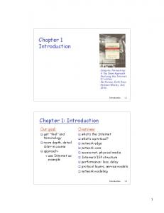
(u1 , ..., ud ) should satisfy Φci and u1 is the ji th real root of R = 0 when (u2 , ..., ud ) is fixed. Remark 52: In Step 3 of Tofind, as in tofind, we only consider those cells homeomorphic to Rd−1 and do not consider those homeomorphic to Rk (k < d − 1). Therefore, if S(u2 , ..., ud ) is a member of the final P olySet and further result when parameter are on both R = 0 and S = 0 is needed, we just put S = 0 into T R and apply above algorithm again. 4.3. DISCOVERER and Examples The algorithms in last subsection have been implemented as a Maple program “DISCOVERER” in our package. There are two main functions, tofind and Tofind, in DISCOVERER. They are applicable to those problems which can be formulated into a parametric sas. Usually, we call tofind first to find a satisfactory condition (see Remark 51) and then, if necessary, call Tofind to find further results when parameter are on some boundaries. The calling sequence in DISCOVERER for a parametric sas T is: tofind ([p1 , · · · , ps ], [g1 , · · · , gr ], [gr+1 , · · · , gt ], [h1 , · · · , hm ], [x1 , · · · , xs ], [u1 , · · · , ud ], α); where α has following three kind of choices: • a non-negative integer b which means the condition for T to have exactly b distinct real solution(s); • a range b..c (b, c are non-negative integers, b < c) which means the condition for T to have b or b + 1 or · · · or c distinct real solutions; • a range b..w (b is a non-negative integer, w a name) which means the condition for T to have more than or equal to b distinct real solutions. Similarly, the calling sequence of Tofind for T and some “boundaries” R1 = 0, ..., Rl = 0 is: Tofind ([p1 , · · · , ps , R1 , · · · , Rl ], [g1 , · · · , gr ], [gr+1 , · · · , gt ], [h1 , · · · , hm ], [x1 , · · · , xs ], [u1 , · · · , ud ], α); where each Ri is a “boundary” which can be a polynomial in parameter obtained by tofind or a constraint polynomial in parameter. Example 53: 15 Which triangles can occur as sections of a regular tetrahedron by planes which separate one vertex from the other three?

March 27, 2006

12:38



yang˙xia3

41

If we let 1, a, b (assume b ≥ a ≥ 1) be the lengths of three sides of the triangle, and x, y, z the distances from the vertex to the three vertexes of the triangle respectively, then, what we need is to find the necessary and sufficient condition that a, b should satisfy for the following system to have real solution(s),  h1 = x2 + y 2 − xy − 1 = 0,    h2 = y 2 + z 2 − yz − a2 = 0,  h = z 2 + x2 − zx − b2 = 0,   3 x > 0, y > 0, z > 0, a − 1 ≥ 0, b − a ≥ 0, a + 1 − b > 0. With our program DISCOVERER, we attack this problem by following two steps. First of all, we type in: tofind ([h1 , h2 , h3 ], [a − 1, b − a], [x, y, z, a + 1 − b], [ ], [x, y, z], [a, b], 1..n); DISCOVERER runs 3 seconds on a PC (Pentium IV/2.8G) with Maple 8,

and outputs FINAL RESULT : The system has required real solution(s) IF AND ONLY IF [0 < R1, 0 < R2] or [0 < R1, R2 < 0, 0 < R3] where R1 = a2 + a + 1 − b2 R2 = a2 − 1 + b − b2 8 8 16 68 241 4 4 68 2 6 R3 = 1 − a2 − b2 + a8 − b6 a2 + b a − b a 3 3 9 27 81 27 68 4 2 68 2 4 2 6 16 8 2 6 46 2 2 − b a − b a − b + b − a + b a 27 27 9 9 9 9 16 4 16 4 46 2 8 46 8 2 68 6 4 68 4 6 + b + a + b a + b a − b a − b a 9 9 9 9 27 27 16 4 8 8 10 2 16 8 4 2 6 6 8 2 10 8 10 + b a − b a + b a − b a − b a − b 9 3 9 9 3 3 8 10 12 12 +b − a + a 3

March 27, 2006

12:38

42


yang˙xia3


PROVIDED THAT : −b + a 6= 0 a − 1 6= 0 b − 1 6= 0 2 a − 1 + b − b2 6= 0 a2 − 1 − b − b2 6= 0 a2 − a + 1 − b2 6= 0 a2 + a + 1 − b2 6= 0 a2 − 1 − ab + b2 6= 0 a2 − 1 + ab + b2 6= 0 R3 6= 0 Folke15 gave a sufficient condition that any triangle with two angles > 60◦ is a possible section. It is easy to see that this condition is equivalent to [R1 > 0, R2 > 0 ]. Now, if parameter a, b are not on the boundaries (that is, R1 = 0, R2 = 0, R3 = 0, a − 1 = 0, b − a = 0, ...), the condition obtained above is already a necessary and sufficient one. But, strictly speaking, to get a necessary and sufficient condition, we have to give the result when a, b are on the boundaries. Thus, we take the second step. If we want to know the result when a, b are on a certain boundary, say R2, we only need to type in Tofind ([h1 , h2 , h3 , R2], [a − 1, b − a], [x, y, z, a + 1 − b], [ ], [x, y, z], [a, b], 1..n); DISCOVERER outputs that (0.44 seconds)

FINAL RESULT: The system has required real solution(s) IF AND ONLY IF [S1 < 0, (2)R2] where S1 = b6 +

56 4 122 3 56 2 b − b + b +1 3 3 3

PROVIDED THAT : b − 1 6= 0 S1 6= 0 [S1 < 0, (2)R2] in the output means a point (a0 , b0 ) in the parametric plane should satisfy that S1 < 0 and a0 is the second root (from the smallest one up) of R2(a, b0 ) = 0. Furthermore, the situation when (a, b) is on

March 27, 2006

12:38



yang˙xia3

43

R2 = 0 ∧ b − 1 = 0 or R2 = 0 ∧ S1 = 0 can be determined by typing in respectively: Tofind ([h1 , h2 , h3 , R2, b−1], [a−1, b−a], [x, y, z, a+1−b], [ ], [x, y, z], [b, a], 1..n); Tofind ([h1 , h2 , h3 , R2, S1], [a−1, b−a], [x, y, z, a+1−b], [ ], [x, y, z], [b, a], 1..n); The outputs both are: The system has 1 real solution! The timings of the computations are 1.13 and 1.44 seconds, respectively. By this way together with some interactive computations, we finally get the condition for the system to have real solution(s): [0 < R1, 0 < R2, R3 ≤ 0, 0 < a − 1, 0 ≤ b − a, 0 < a + 1 − b] or [0 < R1, 0 ≤ R3, 0 ≤ a − 1, 0 ≤ b − a, 0 < a + 1 − b]. Actually, by our algorithm and program, we can do more than the request to this problem. If we type in respectively

Fig. 1.

The complete solution classification of Example 53.

March 27, 2006

12:38


44

yang˙xia3


tofind ([h1 , h2 , h3 ], [a − 1, b − a], [x, y, z, a + 1 − b], [ ], [x, y, z], [a, b], 1); tofind ([h1 , h2 , h3 ], [a − 1, b − a], [x, y, z, a + 1 − b], [ ], [x, y, z], [a, b], 2); tofind ([h1 , h2 , h3 ], [a − 1, b − a], [x, y, z, a + 1 − b], [ ], [x, y, z], [a, b], 3); we will get the condition for the above system to have exactly 1 or 2 or 3 real solution(s) respectively. By this way, we obtain the so-called complete solution classification of this problem, as indicated in Fig. 1. The number (0, 1, 2 or 3) in a certain region indicates the number of distinct real solutions of the system when the parameter a, b are on the region. Example 54: It is well-known that for a triangle there are four tritangent circles (i.e. one inscribed circle and three escribed circles) and a Feuerbach circle (i.e. nine-point-circle) whose radius equals half the circumradius. Given a triangle ABC whose vertices B(1, 0) and C(−1, 0) are fixed and the vertex A(u1 , u2 ) depends on two parameters, we want to find the conditions on u1 , u2 such that there are four, three, two, one or none of the tritangent circles whose radius are smaller than that of Feuerbach circle, respectively. By a routine computation, the system to be dealt with is  2 2 2 2 2 2  f = 16x u2 − (u1 + 2u1 + 1 + u2 )(1 − 2u1 + u1 + u2 ) = 0, 4 2 2 3 2 2 2 i = y u2 + (2 − 2u2 − 2u1 )y + u2 (u1 − 5 + u2 )y + 4u22 y − u32 = 0,  x > 0, x2 − y 2 > 0, where x is the radius of the Feuerbach circle and |y| are the radii of the four tritangent circles. We type in tofind([f, i], [ tofind([f, i], [ tofind([f, i], [ tofind([f, i], [ tofind([f, i], [

], [x, x2 − y 2 ], [ ], [x, x2 − y 2 ], [ ], [x, x2 − y 2 ], [ ], [x, x2 − y 2 ], [ ], [x, x2 − y 2 ], [

], [x, y], [u1 , u2 ], 4); ], [x, y], [u1 , u2 ], 3); ], [x, y], [u1 , u2 ], 2); ], [x, y], [u1 , u2 ], 1); ], [x, y], [u1 , u2 ], 0);

respectively and get the following results (for concision, we rearrange the outputs in a simpler form): FINAL RESULT : The system has 3 (distinct) real solutions IF AND ONLY IF [R1 < 0, R2 > 0, R3 < 0]

March 27, 2006

12:38


yang˙xia3


45

The system has 2 (distinct) real solutions IF AND ONLY IF [R1 > 0] The system has 1 (distinct) real solution IF AND ONLY IF [R1 < 0, R2 < 0] or [R1 < 0, R2 > 0, R3 > 0] The system does not have 0 or 4 real solution(s). where R1 = −7 + 20u62 u21 + 20u22 + 28u21 − 52u21 u22 − 42u41 + 70u42 − 204u62 + 68u42 u21 + 9u82 + 6u42 u41 + 28u61 − 7u81 + 44u41 u22 − 12u22 u61 , 2 2 8 4 4 R2 = 189 + 189u12 1 + 720u2 − 1134u1 − 1977u2 + 2835u1 − 1235u2 6 6 8 6 2 2 2 − 3560u2 − 3780u1 + 2835u1 − 8088u2 u1 − 1968u1 u2 + 2332u42 u21 2 + 558u42 u41 + 672u41 u22 + 2592u22 u61 + 984u62 u61 − 1566u82 u21 − 40u10 2 u1 8 4 6 4 4 6 8 2 8 4 + 135u2 u1 − 2776u2 u1 − 3172u2 u1 − 2928u1 u2 + 1517u1 u2 12 10 10 + 912u22 u10 1 + 15u2 − 168u2 − 1134u1 , 2 16 12 2 2 8 R3 = −63 + 225u14 2 u1 − 63u1 + 4284u1 − 345u2 − 504u1 + 515u2 4 4 6 6 8 6 2 + 4284u1 + 485u2 + 3347u2 − 11592u1 + 15750u1 + 73991u2 u1 − 2851u21 u22 + 23658u42 u21 − 29957u42 u41 + 9791u41 u22 − 4163u22 u61 2 8 4 6 4 + 69174u62 u61 − 125788u82 u21 − 48997u10 2 u1 + 274u2 u1 + 89942u2 u1 4 6 8 2 8 4 2 10 12 4 − 22516u2 u1 − 12163u1 u2 + 36971u1 u2 + 13567u2 u1 + 1031u2 u1 4 10 6 6 8 8 6 − 1974u212 u21 − 2245u10 2 u1 + 1717u2 u1 − 5609u2 u1 − 1052u2 u1 4 12 12 2 6 10 + 995u82 u81 − 7766u42 u10 1 − 875u2 u1 − 3427u1 u2 − 445u2 u1 14 2 12 10 10 14 − 409u1 u2 + 407u2 − 1643u2 − 11592u1 − 15u2 − 504u14 1 ;

PROVIDED THAT : u1 6= 0, u2 6= 0, (u1 + 1)2 + u22 6= 0, (u1 − 1)2 + u22 6= 0, L(u1 , u2 ) = 9 + 84u62 u21 + 84u22 − 36u21 − 116u21 u22 + 54u41 + 166u42 − 140u62 + 132u42 u21 + 25u82 + 102u42 u41 − 36u61 + 9u81 − 20u41 u22 + 52u22 u61 6= 0, R1 6= 0. The total time for executing the five instructions is 87.69 seconds. The non-degenerate condition u2 6= 0 is a premise because otherwise the vertices A, B, C are on a line. Thus (u1 +1)2 +u22 6= 0 and (u1 −1)2 +u22 6= 0

March 27, 2006

46

12:38


yang˙xia3


are verified. Furthermore, it can be easily shown (by DISCOVERER, say) that L(u1 , u2 ) is positive if u1 6= 0 and u2 6= 0. Because we are concerning the complement of the algebraic curve R1 = 0, the only “non-degenerate” condition we need to consider is u1 6= 0. As we did in the preceding example, by typing in Tofind([R2, f, i], [ ], [−R1, x, x2 − y 2 ], [u1 , u2 ], [x, y], [u1 , u2 ], 1); Tofind([R2, f, i], [ ], [−R1, x, x2 − y 2 ], [u1 , u2 ], [x, y], [u1 , u2 ], 3); we get the situation when (u1 , u2 ) is on R2 = 0. Finally, we obtain (1) If u1 = 6 0, The system has 3 (distinct) real solutions IF AND ONLY IF [R1 < 0, R2 > 0, R3 < 0] The system has 2 (distinct) real solutions IF AND ONLY IF [R1 > 0] The system has 1 (distinct) real solution IF AND ONLY IF [R1 < 0, R2 ≤ 0] or [R1 < 0, R2 > 0, R3 > 0] The system does not have 0 or 4 real solution(s); (2) If u1 = 0 (ABC is an isosceles triangle), The system has 2 (distinct) real solutions IF AND ONLY IF [S1 · S2 ≥ 0] The system has 1 (distinct) real solution IF AND ONLY IF [S1 < 0, S2 > 0] The system does not have 0 or 3 or 4 real solution(s) where S1 = u42 − 22u22 − 7, S2 = u22 − 1/3. Note that if u1 = 0 and the system has two distinct real solutions, then one of the solutions is of multiplicity 2 and thus the system has three real solutions indeed. This example was studied in a different way by Guergueb et al.18 . They did not give quantifier-free formulas but illustrated the situation with a sketch figure. Example 55: Give the necessary and sufficient condition for the existence of a triangle with elements a, ha , R, where a, ha , R means the side-length, altitude, and circumradius, respectively.

March 27, 2006

12:38



yang˙xia3

47

Clearly, we need to find the necessary and sufficient condition for the following system to have real solution(s),  f1 = a2 h2a − 4s(s − a)(s − b)(s − c) = 0,      f2 = 2Rha − bc = 0, f3 = 2s − a − b − c = 0,    a > 0, b > 0, c > 0, a + b − c > 0, b + c − a > 0,   c + a − b > 0, R > 0, ha > 0. By the same way as in the preceding examples, we obtain The system has real solution(s) IF AND ONLY IF [0 ≤ R1, 0 ≤ R3] or [0 ≤ R1, R2 ≤ 0, R3 ≤ 0] where 1 R1 = R − a 2 1 R2 = Rha − a2 4 1 1 R3 = − h2a + Rha − a2 . 2 8 The time spent is 0.61 seconds. The condition given by Mitrinovic et al.27 is R1 ≥ 0 ∧ R3 ≥ 0. Now, we know they are wrong and that is only a sufficient condition. Our program, DISCOVERER, is very efficient for solving this kind of problems. By DISCOVERER, we have discovered or rediscovered about 70 such conditions for the existence of a triangle, and found three mistakes in Mitrinovic et al. 27 .

Acknowledgments The authors acknowledge the support provided by NKBRSF(G1998030600). References 1. Aubry, P., Lazard, D., Moreno Maza, M., On the theories of triangular sets, J. Symb. Comput., 28, pp.105–124,1999. 2. Aubry, P., Rouillier, F., Safey El Din, M., Real solving for positive dimensional systems, J. Symb. Comput., 34, pp.543–560, 2002.

March 27, 2006

48

12:38


yang˙xia3


3. Basu, S., Pollack, R., Roy, M.-F., Algorithms in Real Algebraic Geometry, (Algorithms and Computation in Mathematics, Vol. 10), Springer-Verlag, 2003. 4. Becker, T., Weispfenning, V., Gr¨ obner Bases, Springer-Verlag, New York, 1993. 5. Ben-Or, M., Kozen, D., Reif, J., The complexity of elementary algebra and geometry, J. Computer and System Sciences, 32, pp.251–264, 1986. 6. Bottema, O., Dordevic, R. Z., Janic, R. R., Mitrinovic, D. S., Vasic, P. M., Geometric Inequalities, Wolters-Noordhoff Publishing, Groningen, The Netherlands, 1969. 7. Brown, C. W., Simple CAD Construction and Its Applications, J. Symb. Comput., 31, pp.521–547, 2001. obner bases: An algorithmic method in polynomial ideal 8. Buchberger, B., Gr¨ theory in Multidimensional Systems Theory, N.K. Bose ed., Reidel, 1985. 9. Chou, S. C., Gao, X. S., Arnon, D. S., On the mechanical proof of geometry theorems involving inequalities, Advances in Computing Research, 6, JAI Press Inc., pp.139–181, 1992. 10. Collins, G. E., Quantifier elimination for real closed fields by cylindrical algebraic decomposition, in Lecture Notes in Computer Science 33, Springer, 1975. 11. Collins, G. E., Hong, H., Partial cylindical algebraic decomposition for quantifier elimination, J. Symb. Comput., 12, pp.299–328, 1991. 12. Collins, G. E., Loos, R., Real Zeros of Polynomials, in Computer Algebra: Symbolic and Algebraic Computation, Buchberger, B., Collins, G. E., Loos, R. eds., Springer-Verlag, 1983. 13. Davenport, J. H., Heintz, J., Real quantifier elimination is doubly exponential, J. Symb. Comput., 5(1–2), pp.29–35, 1988. 14. Dolzmann, A., Sturm, T., Weispfenning, V., Real quantifier elimination in practice, Algorithmic Algebra and Number Theory, Matzat, B. H., Greuel, G.-M., Hiss, G. eds., Springer-Verlag, pp.221–247, 1998. 15. Folke, E., Which triangles are plane sections of regular tetrahedra?, American Mathematical Monthly, Oct. pp.788–789, 1994. 16. Gonzalez-Vega, L., A combinatorial algorithm solving some quantifier elimination problems, in Quantifier elimination and cylindrical algebraic decomposition, Caviness, B. F., Johnson, J. R. eds., pp.365–375, Springer-Verlag, 1998. 17. Gonzalez-Vega, L., Rouillier, F., Roy, M.-F., Trujillo, G., Symbolic recipes for real solutions, in Some Tapas of Computer Algebra, Cohen, A. M., Cuypers, H., Sterk, H. eds., Springer-Verlag, 1999. 18. Guergueb, A., Mainguené, J., Roy, M-F., Examples of Automatic Theorem Proving in Real Geometry, in ISSAC 1994, pp.20–24, 1994. 19. Hong, H., Quantifier elimination for formulas constrained by quadratic equations, in Proceedings of ISSAC 93, Bronstein, M. ed., pp.264–274, ACM Press, 1993. 20. Janous, W., Problem 1137, Crux Math., 12(1986), 79, 177. 21. Kalkbrener, M., A generalized Euclidean algorithm for computing triangular

March 27, 2006

12:38



22. 23. 24.

25.

26. 27. 28.

29.

30. 31. 32. 33.

34. 35. 36. 37.

38. 39.

yang˙xia3

49

representations of algebraic varieties, J. Symb. Comput., 15, pp.143–167, 1993. Kuang, J. C. Applied Inequalities (in Chinese), 2nd ed., Hunan Educational Publishing House, China, 1993. Liu, B. Q., BOTTEMA,What we see (in Chinese), Tibet People’s Publishing House, Lhasa, 2003. Loos, R., Generalized polynomial remainder sequences, in Computer Algebra: Symbolic and Algebraic Computation, Buchberger, B., Collins, G. E., Loos, R. eds., Springer-Verlag, 1983. Lu, Z. Y., He, B., Luo, Y., Pan, L., An algorithm of real root isolation for polynomial systems, MM Research Preprints, No.20, pp.187–198. MMRC AMSS, Academia Sinica, Beijing, 2001. Ma, S. L., Zheng, Z. M., On a cubic system with eight small-amplitude limit cycles, Appl. Math. Lett., 7, pp.23–27, 1994. Mitrinovic, D. S., Pecaric, J. E., Volenec, V., Recent Advances in Geometric Inequalities, Kluwer Academic Publishers, 1989. Pedersen, P., Roy, M.-F., Szpirglas, A., Counting real zeros in the multivariate case, in Computational Algebraic Geometry, Eyssette, F., Galligo, A. eds., Birkh¨ auser, 1993. Rouillier, F., Solving zero-dimensional systems through the rational univariate representation, Appl. Algebra Engrg. Comm. Comput. 9, pp.433–461, 1999. Rouillier, F., Zimmermann, P., Efficient isolation of a polynomial real roots, Technical Report RR-4113, INRIA, 2001. Shan, Z. (ed.), Geometric Inequality in China (in Chinese), Jiangsu Educational Publishing House, China, 1996. Tarski, A., A Decision Method for Elementary Algebra and Geometry, University of California Press, 1951. Wang, D. K., Zero Decompostion Algorithms for Systems of Polynomial Equations, in Proceedings of the Fourth Asian Symposium on Computer Mathematics (ASCM2000), Gao, X.-S., Wang, D. M. eds., World Scientific, 2000. Wang, D. M., Decomposing polynomial systems into simple systems, J. Symb. Comput., 25, pp.295–314, 1998. Wang, D. M., Computing triangular systems and regular systems, J. Symb. Comput., 30, pp.221–236, 2000. Weispfenning, V., The complexity of linear problems in fields, J. Symb. Comput., 5(1-2), pp.3–27, 1988. Weispfenning, V., Quantifier elimination for real algebra—the cubic case, in Proceedings of the international symposium on Symbolic and algebraic computation (ISSAC 94), pp.258–263, 1994. Weispfenning, V., Quantifier elimination for real algebra—the quadratic case and beyond, Appl. Algebra Engrg. Comm. Comput., 8, pp.85–101, 1997. Weispfenning, V., A new approach to quantifier elimination for real algebra, in Quantifier elimination and cylindrical algebraic decomposition (Linz, 1993), pp.376–392, Texts Monogr. Symbol. Comput., Springer, Vienna, 1998.

March 27, 2006

50

12:38


yang˙xia3


40. Winkler, F., Polynomial Algorithms in Computer Algebra, Springer-Verlag, 1996. 41. Wu, W. T., On zeros of algebraic equations–An application of Ritt principle, Kexue Tongbao, 31, pp.1–5, 1986. 42. Wu, W. T., On a finiteness theorem about problem involving inequalities, Sys. Sci. & Math. Scis., 7, pp.193–200, 1994. 43. Wu, W. T., On global-optimization problems, Proc. ASCM ’98 , Lanzhou University Press, Lanzhou, pp.135–138, 1998. 44. Xia, B. C., Hou, X. R., A complete algorithm for counting real solutions of polynomial systems of equations and inequalities, Computers & Mathematics with Applications, 44, pp.633–642, 2002. 45. Xia, B. C., Yang, L., An algorithm for isolating the real solutions of semialgebraic systems, J. Symb. Comput., 34, pp.461–477, 2002. 46. Xia, B. C., Zhang, T., Real root isolation based on interval arithmetic, Preprint. 47. Yang, L., Recent advances in automated theorem proving on inequalities, J. Comput. Sci. & Technol., 14(5), pp.434–446, 1999. 48. Yang, L., Hou, X. R., Xia, B. C., Automated discovering and proving for geometric inequalities, in Automated Deduction in Geometry (LNAI 1669), Gao, X.-S., Wang, D. M., Yang, L. eds., pp. 30–46, Springer-Verlag, 1999. 49. Yang, L., Hou, X. R., Xia, B. C., A complete algorithm for automated discovering of a class of inequality-type theorems, Science in China, Series F, 44, pp.33–49, 2001. 50. Yang, L., Xia, S. H., An inequality-proving program applied to global optimization, Proceedings of the Asian Technology Conference in Mathematics, W-C. Yang et al (eds.), ATCM, Inc., Blacksburg, pp.40–51, 2000. 51. Yang, L., Xia, S. H., Automated proving for a class of constructive geometric inequalities, Chinese Journal of Computers(in Chinese), 26:(7), pp.769–778, 2003. 52. Yang, L., Zhang, J., A practical program of automated proving for a class of geometric inequalities, in Automated Deduction in Geometry (LNAI 2061), pp.41–57, Springer-Verlag, 2001. 53. Yang, L., Zhang, J. Z., Searching dependency between algebraic equations: An algorithm applied to automated reasoning, Technical Report IC/91/6, International Centre for Theoretical Physics, Trieste, 1991. 54. Yang, L., Zhang, J. Z., Hou, X. R., An efficient decomposition algorithm for geometry theorem proving without factorization, in Proceedings of Asian Symposium on Computer Mathematics 1995, H. Shi and H. Kobayashi ed., pp.33–41, Scientists Incorporated, Japan, 1995. 55. Yang, L., Zhang, J. Z., Hou, X. R., Nonlinear Algebraic Equation System and Automated Theorem Proving (in Chinese), Shanghai Scientific and Technological Education Publishing House, Shanghai, 1996.