spheres, rotations, linear transformations, and more—but in an unfamiliar way. ...
The product involved here is the geometric product, which is the fundamental.
1 WHY GEOMETRIC ALGEBRA?
This book is about geometric algebra, a powerful computational system to describe and solve geometrical problems. You will see that it covers familiar ground—lines, planes, spheres, rotations, linear transformations, and more—but in an unfamiliar way. Our intention is to show you how basic operations on basic geometrical objects can be done differently, and better, using this new framework. The intention of this first chapter is to give you a fair impression of what geometric algebra can do, how it does it, what old habits you will need to extend or replace, and what you will gain in the process.
1.1 AN EXAMPLE IN GEOMETRIC ALGEBRA To convey the compactness of expression of geometric algebra, we give a brief example of a geometric situation, its description in geometric algebra, and the accompanying code that executes this description. It helps us discuss some of the important properties of the computational framework. You should of course read between the lines: you will be able to understand this example fully only at the end of Part II, but the principles should be clear enough now.
1
2
WHY GEOMETRIC ALGEBRA?
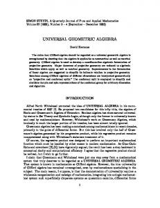
Suppose that we have three points c1 , c2 , c3 in a 3-D space with a Euclidean metric, a line L, and a plane Π. We would like to construct a circle C through the three points, rotate it around the line L, and then reflect the whole scene in the plane Π. This is depicted in Figure 1.1. Here is how geometric algebra encodes this in its conformal model of Euclidean geometry: 1. Circle. The three points are denoted by three elements c1 , c2 , and c3 . The oriented circle through them is C = c1 ∧ c2 ∧ c3 . The ∧ symbol denotes the outer product, which constructs new elements of computation by an algebraic operation that geometrically connects basic elements (in this case, it connects points to form a circle). The outer product is antisymmetric: if you wanted a circle with opposite orientation through these points, it would be −C, which could be made as −C = c1 ∧ c3 ∧ c2 . 2. Rotation. The rotation of the circle C is made by a sandwiching product with an element R called a rotor, as C �→ R C/R.
C c1
RC/R
c3
c2
L
n
M π = p (n`)
p
−π C / π
F i g u r e 1.1: The rotation of a circle C (determined by three points c1 , c2 , c3 ) around a line L, and the reflections of those elements in a plane Π.
CHAPTER 1
SECTION 1.1
AN EXAMPLE IN GEOMETRIC ALGEBRA
3
The product involved here is the geometric product, which is the fundamental product of geometric algebra, and its corresponding division. The geometric product multiplies transformations. It is structure-preserving, because the rotated circle through three points is the circle through the three rotated points: R (c1 ∧ c2 ∧ c3 )/R = (Rc1 /R) ∧ (R c2 /R) ∧ (R c3 /R). Moreover, any element, not just a circle, is rotated by the same rotor-based formula. We define the value of the rotor that turns around the line L below. 3. Line. An oriented line L is also an element of geometric algebra. It can be constructed as a “circle” passing through two given points a1 and a2 and the point at infinity ∞, using the same outer product as in item 1: L = a1 ∧ a2 ∧ ∞. Alternatively, if you have a point on L and a direction vector u for L, you can make the same element as L = a1 ∧ u ∧ ∞. This specifies exactly the same element L by the same outer product, even though it takes different arguments. This algebraic equivalence saves the construction of many specific data types and their corresponding methods for what are geometrically the same elements. The point at infinity ∞ is an essential element of this operational model of Euclidean geometry. It is a finite element of the algebra, with well-defined algebraic properties. 4. Line Rotation. The rotor that represents a rotation around the line L, with rotation angle , is R = exp( L∗ /2). This shows that geometric algebra contains an exponentiation that can make elements into rotation operators. The element L∗ is the dual of the line L. Dualization is an operation that takes the geometric complement. For the line L, its dual can be visualized as the nest of cylinders surrounding it. If you would like to perform the rotation in N small steps, you can interpolate the rotor, using its logarithm to compute R1/N , and applying that n times (we have done so in Figure 1.1, to give a better impression of the transformation). Other transformations, such as general rigid body motions, have logarithms as well in geometric algebra and can therefore be interpolated. 5. Plane. To reflect the whole situation with the line and the circles in a plane Π, we first need to represent that plane. Again, there are alternatives. The most straightforward is to construct the plane with the outer product of three points p1 , p2 , p3 on the plane
4
WHY GEOMETRIC ALGEBRA?
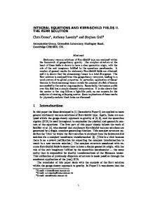
and the point at infinity ∞, as Π = p1 ∧ p2 ∧ p3 ∧ ∞. Alternatively, we can instead employ a specification by a normal vector n and a point p on the plane. This is a specification of the dual plane π ≡ Π∗ , its geometric complement: π = p�(n∞) = n − (p · n) ∞. Here � is a contraction product, used for metric computations in geometric algebra; it is a generalization of the inner product (or dot product) from vectors to the general elements of the algebra. The duality operation above is a special case of the contraction. The change from p to p in the equation is not a typo: p denotes a point, p is its location vector relative to the (arbitrary) origin. The two entities are clearly distinct elements of geometric algebra, though computationally related. 6. Reflection. Either the plane Π or its geometric complement π determine a reflection operator. Points, circles, or lines (in fact, any element X) reflect in the plane in the same way: X �→ − π X/π. Here the reflection plane π, which is an oriented object of geometric algebra, acts as a reflector, again by means of a sandwiching using the geometric product. Note that the reflected circle has the proper orientation in Figure 1.1. As with the rotation in item 2, there is obvious structure preservation: the reflection of the rotated circle is the rotation of the reflected circle (in the reflected line). We can even reflect the rotor to become R� ≡ π exp( L∗ /2)/π = exp(− (−πL∗ /π)/2), which is the rotor around the reflected line, automatically turning in the opposite orientation. 7. Programming. In total, the scene of Figure 1.1 can be generated by a simple C++ program computing directly with the geometric objects in the problem statement, shown in Figure 1.2. The outcome is plotted immediately through the calls to the multivector drawing function draw(). And since it has been fully specified in terms of geometric entities, one can easily change any of them and update the picture. The computations are fast enough to do this and much more involved calculations in real time; the rendering is typically the slowest component. Although the language is still unfamiliar, we hope you can see that this is geometric programming at a very desirable level, in terms of quantities that have a direct geometrical meaning. Each item occurring in any of the computations can be visualized. None of the operations on the elements needed to be specified in terms of their coordinates. Coordinates are only needed when entering the data, to specify precisely which points and lines are to be operated upon. The absence of this quantitative information may suggest that geometric algebra is merely an abstract specification language with obscure operators that merely convey the mathematical logic of geometry. It is much more than that: all expressions are quantitative prescriptions of computations, and can be executed directly. Geometric algebra is a programming language, especially tailored to handle geometry.
CHAPTER 1
SECTION 1.1
AN EXAMPLE IN GEOMETRIC ALGEBRA
5
// l1, l2, c1, c2, c3, p1 are points // OpenGL commands to set color are not shown line L; circle C; dualPlane p; L = unit_r(l1 ^ l2 ^ ni); C = c1 ^ c2 ^ c3; p = p1


![[PDF] Download Geometric Algebra for Computer ... - Google Sites](https://m.moam.info/img/260x300/pdf-download-geometric-algebra-for-computer-google_647840b3097c4786708c9d83.jpg)