Fundamentals of Quantitative Design and Analysis (Chapter 1). 2. Pipelining (Appendix C). 3. Instruction-Level Parallelism and Its Exploitation (Chapter 3). 4.
Computer Architecture Fundamentals of Computer Architecture
Dr. Shadrokh Samavi
What is involved in study of computers
Applications
Technology Programming Languages Interface Design
Evaluation Economics History
Computers
Operating Systems Management
Dr. Shadrokh Samavi
Marketing Fault tolerance Parallelism
Security Communications
2
Course Objective The course objective is to gain the knowledge required to design and analyze high-performance computer systems. Technology
Parallelism
Applications Computer Architecture: • Instruction Set Design • Machine Organization • Hardware
Operating Systems Dr. Shadrokh Samavi
Programming Languages Interface Design
History
3
Topic Coverage Textbook: Hennessy and Patterson, Computer Architecture: A Quantitative Approach, 5th Ed., 2011. 1. 2. 3. 4. 5.
Fundamentals of Quantitative Design and Analysis (Chapter 1) Pipelining (Appendix C) Instruction-Level Parallelism and Its Exploitation (Chapter 3) Memory Hierarchy Design (Chapters 2) Data-Level Parallelism in Vector, SIMD, and GPU Architectures (Chapter 4) 6. Thread-Level Parallelism (Chapter 5) 7. Warehouse-Scale Computers to Exploit Request-Level and Data-Level Parallelism (Chapter 6) Dr. Shadrokh Samavi
4
Some slides are from the instructors’ resources which accompany the 5th and previous editions. Some slides are from David Patterson and Krste Asanovic of UC Berkeley, Israel Koren of UM Amherst, and Milos Prvulovic of Georgia Tech. Sources of some slides are mentioned at the bottom of the page. Please send an email if a name is missing in the above list.
Dr. Shadrokh Samavi
5
1.1 Introduction
Dr. Shadrokh Samavi
6
Semantic Gap Programs running on a computer
Applications (User software)
. . . .
Semantic Gap
Hardware (running the application) Dr. Shadrokh Samavi
7
Semantic Gap • • • • • • • • • •
Applications High level languages Assembly System software Machine language Control Logic blocks Logic gates Transistors Silicon
Dr. Shadrokh Samavi
Problem Algorithm Program/Language Runtime System (VM, OS, MM) ISA (Architecture) Microarchitecture Logic
Circuits Electrons
8
Dr. Shadrokh Samavi
9
Semantic Gap
3 2 1
Dr. Shadrokh Samavi
10
Need for Hierarchy
Dr. Shadrokh Samavi
11
Hierarchy Registers L1 Cache
L2 Cache
Main memory
Hard disk
Dr. Shadrokh Samavi
12
Hierarchy
Intelligence
Knowledge Processing
Information Processing
Data Processing Dr. Shadrokh Samavi
13
• Computer Architecture: The science and art of designing, selecting, and interconnecting hardware components and designing the hardware/software interface to create a computing system that meets functional, performance, energy consumption, cost, and other specific goals. • Traditional definition: “The term architecture is used here to describe the attributes of a system as seen by the programmer, i.e., the conceptual structure and functional behavior as distinct from the organization of the dataflow and controls, the logic design, and the physical implementation.” Gene Amdahl, IBM Journal of R&D, April 1964 Dr. Shadrokh Samavi
14
Introduction
Technology & Design
Rapid rate of improvement of computers has come from: 1. advances in the technology used to build computers 2. innovation in computer design. 1945 – 1970: both forces made a major contribution About 1970 ICs invented and computer designers became largely dependent upon integrated circuit technology. During the 1970s: performance improvement = 25% to 30% per year. Late 1970s: microprocessor invented => 35% performance growth per year. Mass-produced microprocessor => new architectures because: 1. The virtual elimination of assembly language programming reduced the need for object-code compatibility. 2. The creation of standardized, vendor-independent operating systems, such as UNIX and its clone, Linux, lowered the cost and risk of bringing out a new architecture.
Dr. Shadrokh Samavi
15
RISC
RISC (Reduced Instruction Set Computer) architectures in early 1980 caused a sustained performance growth of 50% per year.
Dr. Shadrokh Samavi
16
Hardware Technology 1980
1990
Memory chips
64 KB
4 MB
Clock Rate
1-2 MHz
Hard disks
40 M
1 G
Floppies
.256 M
1.5 M
Dr. Shadrokh Samavi
20-40 MHz
2001 256 MB 700-1200 MHz 40 G 0.5-2 G
17
Processor Perspective • Putting performance growth in perspective: Core i7-4770K processor Cray YMP Type Desktop Supercomputer Year 2016 1988 Clock 3.5GHz 167 MHz MIPS > 1000 MIPS < 50 MIPS Cost $1,200 $1,000,000 Cache 8MB 0.25 KB Memory 16 GB DDR3 256 MB
Dr. Shadrokh Samavi
18
Processor Performance Move to multi-processor
RISC
Constrained by power, instruction-level parallelism, memory latency
Dr. Shadrokh Samavi
19
Source of Performance Improvement • Technology – More transistors per chip ( more transistors smaller transistors shorter paths greater speeds)
• Machine Organization/Implementation – Pipelining, Cache, parallelism, out of order.
• Instruction Set Architecture – Reduced Instruction Set Computers (RISC) – Multimedia extensions – Explicit parallelism
• Compiler technology – Finding more parallelism in code – Greater levels of optimization
Dr. Shadrokh Samavi
20
MIPS64 instruction set architecture formats.
Dr. Shadrokh Samavi
21
Growth in clock rate of microprocessors
Dr. Shadrokh Samavi
22
Intel Core i7 microprocessor die
Dr. Shadrokh Samavi
23
Floorplan of Core i7 die
Dr. Shadrokh Samavi
24
1.2 The Changing Face of Computing
Dr. Shadrokh Samavi
25
1960s: large mainframes for business data processing and large-scale scientific computing. 1970s: minicomputers, timesharing. 1980s: the desktop computer based on microprocessors, replaced timesharing. 1990s: internet, WWW, first PDAs, highperformance digital consumer electronics.
Dr. Shadrokh Samavi
26
Current Trends in Architecture • Cannot continue to leverage InstructionLevel parallelism (ILP) – Single processor performance improvement ended in 2003
• New models for performance: – Data-level parallelism (DLP) – Thread-level parallelism (TLP) – Request-level parallelism (RLP)
• These require explicit restructuring of the application Dr. Shadrokh Samavi
27
Classes of Computers • Personal Mobile Device (PMD) – e.g. start phones, tablet computers – Emphasis on energy efficiency and real-time
• Desktop Computing – Emphasis on price-performance
• Servers – Emphasis on availability, scalability, throughput
• Clusters / Warehouse Scale Computers – Used for “Software as a Service (SaaS)” – Emphasis on availability and price-performance – Sub-class: Supercomputers, emphasis: floating-point performance and fast internal networks
• Embedded Computers – Emphasis: price Dr. Shadrokh Samavi
28
Parallelism • Classes of parallelism in applications: – Data-Level Parallelism (DLP) – Task-Level Parallelism (TLP)
• Classes of architectural parallelism: – Instruction-Level Parallelism (ILP) – Vector architectures/Graphic Processor Units (GPUs) – Thread-Level Parallelism – Request-Level Parallelism
Dr. Shadrokh Samavi
29
Flynn’s Taxonomy • Single instruction stream, single data stream (SISD) • Single instruction stream, multiple data streams (SIMD) – Vector architectures – Multimedia extensions – Graphics processor units
• Multiple instruction streams, single data stream (MISD) – No commercial implementation
• Multiple instruction streams, multiple data streams (MIMD) – Tightly-coupled MIMD – Loosely-coupled MIMD
Dr. Shadrokh Samavi
30
Defining Computer Architecture • “Old” view of computer architecture: – Instruction Set Architecture (ISA) design – i.e. decisions regarding: » registers, memory addressing, addressing modes, instruction operands, available operations, control flow instructions, instruction encoding
• “Real” computer architecture: – Specific requirements of the target machine – Design to maximize performance within constraints: cost, power, and availability – Includes ISA, microarchitecture, hardware Dr. Shadrokh Samavi
31
Trends in Technology • Integrated circuit technology – Transistor density: 35%/year – Die size: 10-20%/year – Integration overall: 40-55%/year
• DRAM capacity: 25-40%/year (slowing) • Flash capacity: 50-60%/year – 15-20X cheaper/bit than DRAM
• Magnetic disk technology: 40%/year – 15-25X cheaper/bit then Flash – 300-500X cheaper/bit than DRAM Dr. Shadrokh Samavi
32
Bandwidth and Latency • Bandwidth or throughput – Total work done in a given time – 10,000-25,000X improvement for processors – 300-1200X improvement for memory and disks
• Latency or response time – Time between start and completion of an event – 30-80X improvement for processors – 6-8X improvement for memory and disks
Dr. Shadrokh Samavi
33
Bandwidth and Latency
Log-log plot of bandwidth and latency milestones Dr. Shadrokh Samavi
34
Transistors and Wires • Feature size
– Minimum size of transistor or wire in x or y dimension – 10 microns in 1971 to .032 microns in 2011 – Transistor performance scales linearly » Wire delay does not improve with feature size!
– Integration density scales quadratically
Dr. Shadrokh Samavi
35
Cost, Price and their Trends
Dr. Shadrokh Samavi
36
Trends in Cost • Cost driven down by learning curve
– Yield • DRAM: price closely tracks cost • Microprocessors: price depends on volume
– 10% less for each doubling of volume
Dr. Shadrokh Samavi
37
Learning Curve production costs
volume
Years time to introduce new product the learning curve— manufacturing costs decrease over time. The learning curve itself is best measured by change in yield— the percentage of manufactured devices that survives the testing procedure.
Dr. Shadrokh Samavi
38
The learning curve at work
Prices of six generations of DRAMs Dr. Shadrokh Samavi
39
Silicon to chip
Dr. Shadrokh Samavi
40
Intel Core i7 Wafer
• 300mm wafer, 280 chips, 32nm technology • Each chip is 20.7 x 10.5 mm Dr. Shadrokh Samavi
41
Integrated Circuit Cost • Integrated circuit
•
This Bose-Einstein formula is an empirical model developed by looking at the yield of many manufacturing lines [Sydow 2006]. Wafer yield accounts for wafers that are completely bad and so need not be tested. For simplicity, we'll just assume the wafer yield is 100%.Defects per unit area is a measure of the random manufacturing defects that occur. In 20I0, the value was typically 0.1 to 0.3 defects per square inch, or 0.016 to 0.057 defects per square centimeter, for a 40 nm process, as it depends on the maturity of the process (recall the learning curve, mentioned earlier). Finally, N is a parameter called the process-complexity factor, a measure of manufacturing difficulty. For 40 nm processes in 2010, N ranged from 11.5 to 15.5.
Dr. Shadrokh Samavi
42
Integrated Circuits Costs
Defect Density Trends
Dr. Shadrokh Samavi
43
Defect Density Trends
Dr. Shadrokh Samavi
44
Yield Manufacturing Defects
13/16 working chips 81.25% yield
Dr. Shadrokh Samavi
1/4 working chips 25.0% yield
45
Yield Assuming $250 per wafer: $5.92 per die $58.82 per die
52 die, 81.25% yield 42.25 working parts / wafer
Dr. Shadrokh Samavi
17 die, 25.0% yield 4.25 working parts / wafer
46
Dependability 1. Service accomplishment, where the service is delivered as specified 2. Service interruption, where the delivered service is different from the SLA Service Level Agreements (SLA) Module reliability: measure of mean time to failure (MTTF) Module availability is a measure of the service accomplishment Module availability= MTTF
MTTR
MTTF (MTTF + MTTR) MTTF
MTTR: mean time to repair
MTTR
time
Dr. Shadrokh Samavi
47
Example: Assume a disk subsystem with the following components and MTTF: 10 disks, each rated at 1,000,000-hour MTTF 1 SCSI controller, 500,000-hour MTTF 1 power supply, 200,000-hour MTTF 1 fan, 200,000-hour MTTF 1 SCSI cable, 1,000,000-hour MTTF
FIT: failure in time, number of failures in one billion hours
Dr. Shadrokh Samavi
48
Technology Trends
Dr. Shadrokh Samavi
49
Recent Microprocessor Trends
Dr. Shadrokh Samavi
50
Dr. Shadrokh Samavi
51
Processor
Transistor count
Date of introduction
Manufacturer
Process
Area
Core i7 (Quad)
731,000,000
2008
Intel
45 nm
263 mm²
POWER6
789,000,000
2007
IBM
65 nm
341 mm²
Six-Core Opteron 904,000,000 2400
2009
AMD
45 nm
Six-Core Core i7
1,170,000,000
2010
Intel
32 nm
Dual-Core Itanium 2
1,700,000,000
2006
Intel
90 nm
Six-Core Xeon 7400
1,900,000,000
2008
Intel
45 nm
Quad-Core Itanium Tukwila
2,000,000,000
2010
Intel
65 nm
8-Core Xeon Nehalem-EX
2,300,000,000
2010
Intel
45 nm
Dr. Shadrokh Samavi
596 mm²
52
Intel x86 Evolution: Milestones Name • 8086
Date 1978
Transistors 29K
MHz 5-10
– First 16-bit Intel processor. Basis for IBM PC & DOS – 1MB address space • 386
1985
275K
16-33
– First 32 bit Intel processor , referred to as IA32 – Added “flat addressing”, capable of running Unix • Pentium 4E
2004
125M
2800-3800
– First 64-bit Intel x86 processor, referred to as x86-64 • Core 2
2006
291M
1060-3333
– First multi-core Intel processor • Core i7
2008
– Four cores
Dr. Shadrokh Samavi
731M
1600-4400
Intel x86 Processors • Machine Evolution
– – – – – – – –
386 Pentium Pentium/MMX PentiumPro Pentium III Pentium 4 Core 2 Duo Core i7
1985 1993 1997 1995 1999 2000 2006 2008
0.3M 3.1M 4.5M 6.5M 8.2M 42M 291M 731M
• Added Features
– – – –
Instructions to support multimedia operations Instructions to enable more efficient conditional operations Transition from 32 bits to 64 bits More cores
Dr. Shadrokh Samavi
Intel x86 Processors • Past Generations
– – – –
1st 1st 1st 1st
Pentium Pro Pentium III Pentium 4 Core 2 Duo
1995 1999 2000 2006
• Recent Generations
1. Nehalem 2.
3. 4. 5. 6. 7. –
Process technology
600 250 180 65
nm nm nm nm
Process technology dimension = width of narrowest wires (10 nm ≈ 100 atoms wide)
2008 45 nm Sandy Bridge 2011 32 nm Ivy Bridge 2012 22 nm Haswell 2013 22 nm Broadwell 2014 14 nm Skylake 2015 14 nm Kaby Lake 2016(mobile) 2017(desktop) Cannonlake 2018 10 nm
Dr. Shadrokh Samavi
14 nm
2016 State of the Art: Skylake • Mobile Model: Core i7
– 2.6-2.9 GHz – 45 W • Desktop Model: Core i7
– Integrated graphics – 2.8-4.0 GHz – 35-91 W • Server Model: Xeon
– – – –
Integrated graphics Multi-socket enabled 2-3.7 GHz 25-80 W Dr. Shadrokh Samavi
Intel Core i7 "Skylake" (14 nm) Clock frequency: 4 GHz Technology: 14nm Cores: 4 Thermal Design Power: 95 W Two threads per core L1 cache: 4× 32 KB + 4× 32 KB L2 cache: 4 × 256 KB L3 cache: 8 MB Price: $340 August 2015 http://en.wikipedia.org/wiki/List_of_Intel_Core_i7_microprocessors
Dr. Shadrokh Samavi
57
Moore’s Law & Power Dissipation
Dr. Shadrokh Samavi
58
Power and Energy
Dr. Shadrokh Samavi
59
Power and Energy • Problem: Get power in, get power out • Thermal Design Power (TDP) – Characterizes sustained power consumption – Used as target for power supply and cooling system – Lower than peak power, higher than average power consumption
• Clock rate can be reduced dynamically to limit power consumption • Energy per task is often a better measurement
Dr. Shadrokh Samavi
60
Dynamic Energy and Power • Dynamic energy Transistor switch from 0 -> 1 or 1 -> 0 ½ x Capacitive load x Voltage2
• Dynamic power ½ x Capacitive load x Voltage2 x Frequency switched
• Reducing clock rate reduces power, not energy
Dr. Shadrokh Samavi
61
Power Trends
• In CMOS IC technology
Power Capacitive load Voltage 2 Frequency ×30
Dr. Shadrokh Samavi
5V → 1V
×1000
62
Reducing Power • Techniques for reducing power:
– Do nothing well – Dynamic Voltage-Frequency Scaling – Low power state for DRAM, disks – Overclocking, turning off cores
Dr. Shadrokh Samavi
63
Static Power • Static power consumption
– Currentstatic x Voltage – Scales with number of transistors – To reduce: power gating
Dr. Shadrokh Samavi
64
Consumption of Power in Laptops
Dr. Shadrokh Samavi
65
Server Farms • Internet data centers are like heavy-duty factories – e.g. small Datacenter 25,000 sq.feet, 8000 servers, 2MegaWatts – Intergate Datacenter, Tukwila, WA: 1.5 Mill. Sq.Ft, ~500 MW – Wants lowest net cost per server per sq foot of data center space • Cost driven by: – Racking height – Cooling air flow – Power delivery – Maintenance ease (access, weight) – 25% of total cost due to power
Prof. David Brooks, Harvard University
Dr. Shadrokh Samavi
66
Measuring and Reporting Performance
Dr. Shadrokh Samavi
67
Measuring Performance • Typical performance metrics: – Response time – Throughput
• Speedup of X relative to Y – Execution timeY / Execution timeX
• Execution time
– Wall clock time: includes all system overheads – CPU time: only computation time
• Benchmarks – – – –
Kernels (e.g. matrix multiply) Toy programs (e.g. sorting) Synthetic benchmarks (e.g. Dhrystone) Benchmark suites (e.g. SPEC06fp, TPC-C) Dr. Shadrokh Samavi
68
Applications -> Requirements -> Designs • scientific: weather prediction, molecular modeling • need: large memory, floating-point arithmetic • examples: CRAY-1, T3E, IBM DeepBlue, BlueGene
• commercial: inventory, payroll, web serving, e-commerce • need: integer arithmetic, high I/O • examples: SUN SPARCcenter, Enterprise, AlphaServer GS320 • desktop: multimedia, games, entertainment • need: high data bandwidth, graphics • examples: Intel Pentium4, IBM Power5, Motorola PPC 620 • mobile: laptops • need: low power (battery), good performance • examples: Intel Mobile Pentium 4, Transmeta TM5400
• embedded: cell phones, automobile engines, door knobs • need: low power (battery + heat), low cost • examples: Compaq/Intel StrongARM, X-Scale, Transmeta TM3200 Dr. Shadrokh Samavi
69
Importance of servers’ availability
Dr. Shadrokh Samavi
70
Computing Market
1.8 billion PMDs (90% cell phones) 350 million desktops 20 million servers 19 billion embedded processors sold in 2010 Dr. Shadrokh Samavi
71
Dr. Shadrokh Samavi
72
Dr. Shadrokh Samavi
73
Dr. Shadrokh Samavi
74
Example for Performance Plane
DC to Paris
Speed
Passengers
Throughput (pmph)
Boeing 747
6.5 hours
610 mph
470
286,700
Concorde
3 hours
1350 mph
132
178,200
Douglas DC-8-50
7.4 hours
544
146
79,424
• Time to run the task (Execution Time) – Execution time, response time, latency
• Tasks per day, hour, week, sec, ns … (Performance) – Throughput, bandwidth
Dr. Shadrokh Samavi
75
Performance and Execution Time
Execution time and performance are reciprocals ExTime(Y) ExTime(X)
Performance(X)
= Performance(Y)
Dr. Shadrokh Samavi
76
Performance Terminology “X is n% faster than Y” means: ExTime(Y) --------- = ExTime(X)
Performance(X) -------------Performance(Y)
=
1
+
n ----100
n = 100(Performance(X) - Performance(Y)) Performance(Y) n = 100(ExTime(Y) - ExTime(X)) ExTime(X) Example: Y takes 15 seconds to complete a task, X takes 10 seconds. What % faster is X? Dr. Shadrokh Samavi
77
Example
Example: Y takes 15 seconds to complete a task, X takes 10 seconds. What % faster is X? n = 100(ExTime(Y) - ExTime(X)) ExTime(X) n = 100(15 - 10) 10 n = 50% Dr. Shadrokh Samavi
78
Benchmarks:
Programs to Evaluate Processor Performance
1. Real applications— compilers for C, processing software like Word, and applications like Photoshop.
textother
2. Modified (or scripted) applications— 3. Kernels—key pieces from real programs 4. Toy benchmarks— Puzzle, and Quicksort 5. Synthetic benchmarks— not even pieces of real programs.
Dr. Shadrokh Samavi
79
Benchmarks • Benchmark mistakes – – – – – – –
Only average behavior represented in test workload Loading level controlled inappropriately Caching effects ignored Buffer sizes not appropriate Ignoring monitoring overhead Not ensuring same initial conditions Collecting too much data but doing too little analysis
• Benchmark tricks – Compiler wired to optimize the workload – Very small benchmarks used – Benchmarks manually translated to optimize performance Dr. Shadrokh Samavi
80
SPEC: Standard Performance Evaluation Cooperative • First Round SPEC CPU89 – 10 programs yielding a single number
• Second Round SPEC CPU92 – SPEC CINT92 (6 integer programs) and SPEC CFP92 (14 floating point programs) – Compiler flags can be set differently for different programs
• Third Round SPEC CPU95 – new set of programs: SPEC CINT95 (8 integer programs) and SPEC CFP95 (10 floating point) – Single flag setting for all programs
• Fourth Round SPEC CPU2000 – new set of programs: SPEC CINT2000 (12 integer programs) and SPEC CFP2000 (14 floating point) – Single flag setting for all programs – Programs in C, C++, Fortran 77, and Fortran 90
Dr. Shadrokh Samavi
81
Measuring Performance
1. 2. 3. 4.
SPEC2017 Integer Of the 12 SPEC2017 integer programs, 5 are written in C, 4 in C++, and 1 in Fortran
Floating point For the floating-point programs the split is 3 in FORTRAN, 4 in C++, 3 in C, and 4 in mixed C and Fortran.
Dr. Shadrokh Samavi
Perl interpreter GNU C compiler Route planning Discrete Event simulation - computer network 5. XML to HTML conversion via XSLT 6. Video compression 7. Artificial Intelligence: (Chess) 8. Artificial Intelligence: Monte Carlo tree search 9. Artificial Intelligence: (Sudoku) 10.General data compression 1. Explosion modeling 2. Physics: relativity 3. Molecular dynamics 4. Biomedical imaging: 5. Ray tracing 6. Fluid dynamics 7. Weather forecasting 8. 3D rendering and animation 9. Atmosphere modeling 10.Wide-scale ocean modeling 11.Image manipulation 12.Molecular dynamics 13.Computational Electromagnetics 14.Regional ocean modeling
82
Other SPEC Benchmarks • JVM98: – Measures performance of Java Virtual Machines
• SFS97: – Measures performance of network file server (NFS) protocols
• Web99: – Measures performance of World Wide Web applications
• HPC96: – Measures performance of large, industrial applications
• APC, MEDIA, OPC – Measure performance of graphics applications
• SPEC Cloud_IaaS 2016: ‒ Cloud
http://www.spec.org Dr. Shadrokh Samavi
83
Comparing Performance
Computer A
Computer B
Computer C
Program P1 (secs)
1
10
20
Program P2 (secs)
1000
100
20
Total time (secs)
1001
110
40
Dr. Shadrokh Samavi
Comparing Performance An average of the execution times is the arithmetic mean: weighted arithmetic mean:
Average normalized execution time is the geometric mean:
Dr. Shadrokh Samavi
85
In May 1995, the SPECopc project group decided to adopt a weighted geometric mean as the single composite metric for each viewset. What is a Weighted Geometric Mean? Above is the formula for determining a weighted geometric mean, where "n" is the number of individual tests in a viewset, and "w" is the weight of each individual test, expressed as a number between 0.0 and 1.0. (A test with a weight of "10.0%" is a "w" of 0.10. Note the sum of the weights of the individual tests must equal 1.00.) http://www.spec.org/gpc/opc.static/geometric.html
Dr. Shadrokh Samavi
86
Comparing Performance Normalized to A AB
Normalized to B
Normalized to C
C
A
B
C
AB
20.0
0.1
1.0
2.0
0.05
10.0
1.0
0.2
Program P1
1.0
10.0
Program P2
1.0
0.1
0.02
Arithmetic mean
1.0
5.05
10.01
5.05
1.0
Geometric mean
1.0
1.0
0.63
1.0
Total time
1.0
0.11
0.04
9.1
Computer A
C 0.5
1.0
50.0
5.0
1.0
1.1
25.03
2.75
1.0
1.0
0.63
1.58
1.58
1.0
1.0
0.36
25.03
2.75
1.0
Computer B
Computer C
Program P1 (secs)
1
10
20
Program P2 (secs)
1000
100
20
Total time (secs)
1001
110
40
Dr. Shadrokh Samavi
87
Quantitative Principles of Computer Design
Dr. Shadrokh Samavi
88
Principles of Computer Design • Take Advantage of Parallelism – e.g. multiple processors, disks, memory banks, pipelining, multiple functional units
• Principle of Locality – Reuse of data and instructions
• Focus on the Common Case – Amdahl’s Law
Dr. Shadrokh Samavi
89
Principles of Computer Design • The Processor Performance Equation
Dr. Shadrokh Samavi
90
Principles of Computer Design • Different instruction types having different CPIs
Dr. Shadrokh Samavi
91
Amdahl's Law Speedup due to enhancement E: ExTime w/o E Speedup(E) = ------------- = ExTime w/ E
Performance w/ E ----------------------Performance w/o E
Suppose that enhancement E accelerates a fraction Fractionenhanced of the task by a factor Speedupenhanced, and the remainder of the task is unaffected. What are the new execution time and the overall speedup due to the enhancement? Dr. Shadrokh Samavi
92
Amdahl's Law
ExTimenew = ExTimeold x (1 - Fractionenhanced) + Fractionenhanced Speedupenhanced
Speedupoverall =
ExTimeold ExTimenew
=
1 (1 - Fractionenhanced) + Fractionenhanced Speedupenhanced
Dr. Shadrokh Samavi
93
Example of Amdahl’s Law
• Floating point instructions improved to run 2X; but only 10% of the time was spent on these instructions. ExTimenew = Speedupoverall =
Dr. Shadrokh Samavi
94
Example of Amdahl’s Law
• Floating point instructions improved to run 2X; but only 10% of the time was spent on these instructions. ExTimenew = ExTimeold x (0.9 + .1/2) = 0.95 x ExTimeold Speedupoverall = ExTimenew = 1 ExTimeold 0.95
= 1.053
• The new machine is 5.3% faster for this mix of instructions. Dr. Shadrokh Samavi
95
Dr. Shadrokh Samavi
96
Make The Common Case Fast • All instructions require an instruction fetch, only a fraction require a data fetch/store. – Optimize instruction access over data access
• Programs exhibit locality - 90% of time in 10% of code - Temporal Locality (items referenced recently)
- Spatial Locality (items referenced nearby) • Access to small memories is faster – Provide a storage hierarchy such that the most frequent accesses are to the smallest (closest) memories.
Reg's
Cache
Memory
Dr. Shadrokh Samavi
Disk / Tape
97
Aspects of CPU Performance CPU time
= Seconds Program
= Instructions x Program
Inst Count
CPI
X
X
Compiler
X
X
Inst. Set.
X
X
Organization
X
Dr. Shadrokh Samavi
x Seconds
Instruction
Program
Technology
Cycles
Cycle
Clock Rate
X X
98
Marketing Metrics MIPS = Instruction Count / Time * 10^6 = Clock Rate / CPI * 10^6 • Not effective for machines with different instruction sets • Not effective for programs with different instruction mixes • Uncorrelated with performance
MFLOPs = FP Operations / Time * 10^6 • Machine dependent • Often not where time is spent •Peak - maximum able to achieve •Native - average for a set of benchmarks •Relative - compared to another platform
Dr. Shadrokh Samavi
Normalized MFLOPS: add,sub,compare,mult 1 divide, sqrt
4
exp, sin, . . .
8
99
Suppose we have made the following measurements: Frequency of FP operations () = 25% Average CPI of FP operations = 4.0 Average CPI of other instructions = 1.33 Frequency of FPSQR= 2% CPI of FPSQR = 20 Assume that the two design alternatives are to decrease the CPI of FPSQR to 2 or to decrease the average CPI of all FP operations to 2.5. Compare these two design alternatives using the CPU performance equation.
Dr. Shadrokh Samavi
100
Dr. Shadrokh Samavi
101
Conclusions on Performance • A fundamental rule in computer architecture is to make the common case fast. • The most accurate measure of performance is the execution time of representative real programs (benchmarks). • Execution time is dependent on the number of instructions per program, the number of cycles per instruction, and the clock rate. • When designing computer systems, both cost and performance need to be taken into account.
Dr. Shadrokh Samavi
102
Performance and Price-Performance
Dr. Shadrokh Samavi
103
Performance and price-performance 1. desktop systems using the SPEC CPU benchmarks 2. servers using TPC-C as the benchmark
3. embedded processors using EEMBC as the benchmark.
Dr. Shadrokh Samavi
104
Six different systems from three vendors using different microprocessors showing the processor, its clock rate, and the selling price.
Dr. Shadrokh Samavi
105
Performance and price-performance
Dr. Shadrokh Samavi
106
(OLTP) servers:
Dr. Shadrokh Samavi
Online Transaction Processing
107
Online Transaction Processing (OLTP) servers
TPM: transactions per minute
Dr. Shadrokh Samavi
108