In general, we shall study a system of m linear equations of the form a11x1 + a12x2 + . ...... the array (2), with m row
LINEAR ALGEBRA W W L CHEN c
W W L Chen, 1982, 2008.
This chapter originates from material used by the author at Imperial College, University of London, between 1981 and 1990. It is available free to all individuals, on the understanding that it is not to be used for financial gain, and may be downloaded and/or photocopied, with or without permission from the author. However, this document may not be kept on any information storage and retrieval system without permission from the author, unless such system is not accessible to any individuals other than its owners.
Chapter 1 LINEAR EQUATIONS
1.1. Introduction Example 1.1.1. Try to draw the two lines 3x + 2y = 5, 6x + 4y = 5. It is easy to see that the two lines are parallel and do not intersect, so that this system of two linear equations has no solution. Example 1.1.2. Try to draw the two lines 3x + 2y = 5, x + y = 2. It is easy to see that the two lines are not parallel and intersect at the point (1, 1), so that this system of two linear equations has exactly one solution. Example 1.1.3. Try to draw the two lines 3x + 2y = 5, 6x + 4y = 10. It is easy to see that the two lines overlap completely, so that this system of two linear equations has infinitely many solutions. Chapter 1 : Linear Equations
page 1 of 31
c
Linear Algebra
W W L Chen, 1982, 2008
In these three examples, we have shown that a system of two linear equations on the plane R2 may have no solution, one solution or infinitely many solutions. A natural question to ask is whether there can be any other conclusion. Well, we can see geometrically that two lines cannot intersect at more than one point without overlapping completely. Hence there can be no other conclusion. In general, we shall study a system of m linear equations of the form a11 x1 + a12 x2 + . . . + a1n xn = b1 , a21 x1 + a22 x2 + . . . + a2n xn = b2 , .. .
(1)
am1 x1 + am2 x2 + . . . + amn xn = bm , with n variables x1 , x2 , . . . , xn . Here we may not be so lucky as to be able to see geometrically what is going on. We therefore need to study the problem from a more algebraic viewpoint. In this chapter, we shall confine ourselves to the simpler aspects of the problem. In Chapter 6, we shall study the problem again from the viewpoint of vector spaces. If we omit reference to the variables, then system (1) can be represented by the array
a11 a21 . ..
a12 a22 .. .
am1
... ...
am2
...
a1n a2n .. .
amn
b1 b2 .. .
(2)
bm
of all the coefficients. This is known as the augmented matrix of the system. Here the first row of the array represents the first linear equation, and so on. We also write Ax = b, where
a11 a21 A= ...
am1
a12 a22 .. .
am2
...
b1 b2 b= ...
a1n a2n .. .
... ...
and
amn
bm
represent the coefficients and
x1 x2 x= ... xn
represents the variables. Example 1.1.4. The array
1 0 2
3 1 4
1 1 0
5 2 7
1 1 1
5 4 3
(3)
represents the system of 3 linear equations x1 + 3x2 + x3 + 5x4 + x5 = 5, x2 + x3 + 2x4 + x5 = 4, 2x1 + 4x2 Chapter 1 : Linear Equations
(4)
+ 7x4 + x5 = 3, page 2 of 31
c
Linear Algebra
W W L Chen, 1982, 2008
with 5 variables x1 , x2 , x3 , x4 , x5 . We can also write
1 0 2
3 1 4
1 1 0
5 2 7
x1 1 x2 5 1 x3 = 4 . 1 x4 3 x5
1.2. Elementary Row Operations Let us continue with Example 1.1.4. Example 1.2.1. Consider the array (3). Let us interchange the first and second rows to obtain 0 1 1 2 1 4 1 3 1 5 1 5. 2 4 0 7 1 3 Then this represents the system of equations x2 + x3 + 2x4 + x5 = 4, x1 + 3x2 + x3 + 5x4 + x5 = 5, 2x1 + 4x2
(5)
+ 7x4 + x5 = 3,
essentially the same as the system (4), the only difference being that the first and second equations have been interchanged. Any solution of the system (4) is a solution of the system (5), and vice versa. Example 1.2.2. Consider the array (3). Let us add 2 times the second row to the first row to obtain 1 5 3 9 3 13 0 1 1 2 1 4 . 2 4 0 7 1 3 Then this represents the system of equations x1 + 5x2 + 3x3 + 9x4 + 3x5 = 13, x2 + x3 + 2x4 + x5 = 4, 2x1 + 4x2
(6)
+ 7x4 + x5 = 3,
essentially the same as the system (4), the only difference being that we have added 2 times the second equation to the first equation. Any solution of the system (4) is a solution of the system (6), and vice versa. Example 1.2.3. Consider the array (3). Let us multiply the second row by 2 to obtain 1 3 1 5 1 5 0 2 2 4 2 8. 2 4 0 7 1 3 Then this represents the system of equations x1 + 3x2 + x3 + 5x4 + x5 = 5, 2x2 + 2x3 + 4x4 + 2x5 = 8, 2x1 + 4x2 Chapter 1 : Linear Equations
(7)
+ 7x4 + x5 = 3, page 3 of 31
c
Linear Algebra
W W L Chen, 1982, 2008
essentially the same as the system (4), the only difference being that the second equation has been multiplied through by 2. Any solution of the system (4) is a solution of the system (7), and vice versa. In the general situation, it is not difficult to see the following. PROPOSITION 1A. (ELEMENTARY ROW OPERATIONS) Consider the array (2) corresponding to the system (1). (a) Interchanging the i-th and j-th rows of (2) corresponds to interchanging the i-th and j-th equations in (1). (b) Adding a multiple of the i-th row of (2) to the j-th row corresponds to adding the same multiple of the i-th equation in (1) to the j-th equation. (c) Multiplying the i-th row of (2) by a non-zero constant corresponds to multiplying the i-th equation in (1) by the same non-zero constant. In all three cases, the collection of solutions to the system (1) remains unchanged. Let us investigate how we may use elementary row operations to help us solve a system of linear equations. As a first step, let us continue again with Example 1.1.4. Example 1.2.4. Consider again the system of linear equations x1 + 3x2 + x3 + 5x4 + x5 = 5, x2 + x3 + 2x4 + x5 = 4, 2x1 + 4x2
(8)
+ 7x4 + x5 = 3,
represented by the array
1 0 2
3 1 4
1 1 0
5 2 7
1 1 1
5 4. 3
(9)
Let us now perform elementary row operations on the array (9). At this point, do not worry if you do not understand why we are taking the following steps. Adding −2 times the first row of (9) to the third row, we obtain
1 0 0
3 1 −2
1 1 −2
5 2 −3
1 1 −1
5 4 . −7
From here, we add 2 times the second row to the third row to obtain
1 0 0
3 1 0
1 1 0
5 2 1
1 1 1
5 4. 1
(10)
Next, we add −3 times the second row to the first row to obtain
1 0 0 1 0 0
−2 1 0
−1 2 1
−2 1 1
−7 4 . 1
Next, we add the third row to the first row to obtain
1 0 0 Chapter 1 : Linear Equations
0 1 0
−2 1 0
0 −1 −6 2 1 4 . 1 1 1 page 4 of 31
c
Linear Algebra
Finally, we add −2 times the third to row to 1 0 0 1 0 0
the second row to obtain −2 0 −1 −6 1 0 −1 2 . 0 1 1 1
W W L Chen, 1982, 2008
(11)
We remark here that the array (10) is said to be in row echelon form, while the array (11) is said to be in reduced row echelon form – precise definitions will follow in Sections 1.5–1.6. Let us see how we may solve the system (8) by using the arrays (10) or (11). First consider (10). Note that this represents the system x1 + 3x2 + x3 + 5x4 + x5 = 5, x2 + x3 + 2x4 + x5 = 4,
(12)
x4 + x5 = 1. First of all, take the third equation x4 + x5 = 1. If we let x5 = t, then x4 = 1 − t. Substituting these into the second equation, we obtain (you must do the calculation here) x2 + x3 = 2 + t. If we let x3 = s, then x2 = 2 + t − s. Substituting all these into the first equation, we obtain (you must do the calculation here) x1 = −6 + t + 2s. Hence x = (x1 , x2 , x3 , x4 , x5 ) = (−6 + t + 2s, 2 + t − s, s, 1 − t, t) is a solution of the system (12) for every s, t ∈ R. In view of Proposition 1A, these are also precisely the solutions of the system (8). Alternatively, consider (11) instead. Note that this represents the system x1
− 2x3 x2 + x3
− x5 = −6, − x5 =
2,
x4 + x5 =
1.
(13)
First of all, take the third equation x4 + x5 = 1. If we let x5 = t, then x4 = 1 − t. Substituting these into the second equation, we obtain (you must do the calculation here) x2 + x3 = 2 + t. If we let x3 = s, then x2 = 2 + t − s. Substituting all these into the first equation, we obtain (you must do the calculation here) x1 = −6 + t + 2s. Hence x = (x1 , x2 , x3 , x4 , x5 ) = (−6 + t + 2s, 2 + t − s, s, 1 − t, t) Chapter 1 : Linear Equations
page 5 of 31
c
Linear Algebra
W W L Chen, 1982, 2008
is a solution of the system (13) for every s, t ∈ R. In view of Proposition 1A, these are also precisely the solutions of the system (8). However, if you have done the calculations as suggested, you will notice that the calculation is easier for the system (13) than for the system (12). This is clearly a case of the array (11) in reduced row echelon form having more 0’s than the array (10) in row echelon form, so that the system (13) has fewer non-zero coefficients than the system (12).
1.3. Row Echelon Form Definition. A rectangular array of numbers is said to be in row echelon form if the following conditions are satisfied: (1) The left-most non-zero entry of any non-zero row has value 1. These are called the pivot entries. (2) All zero rows are grouped together at the bottom of the array. (3) The pivot entry of a non-zero row occurring lower in the array is to the right of the pivot entry of a non-zero row occurring higher in the array. Next, we investigate how we may reduce a given array to row echelon form. We shall illustrate the ideas by working on an example. Example 1.3.1. Consider the array
0 0 0 0
0 2 1 1
5 4 2 2
0 7 3 4
15 1 0 1
5 3 . 1 2
Step 1: Locate the left-most non-zero column and cover all columns to the left of this column (in our illustration here, × denotes an entry that has been covered). We now have
× × × ×
0 2 1 1
5 4 2 2
0 7 3 4
15 1 0 1
5 3 . 1 2
Step 2: Consider the part of the array that remains uncovered. By interchanging rows if necessary, ensure that the top-left entry is non-zero. So let us interchange rows 1 and 4 to obtain × 1 2 4 1 2 × 2 4 7 1 3 . × 1 2 3 0 1 × 0 5 0 15 5 Step 3: If the top entry on the left-most uncovered column is a, then we multiply the top uncovered row by 1/a to ensure that this entry becomes 1. So let us divide row 1 by 1 to obtain
× × × ×
1 2 1 0
2 4 2 5
4 7 3 0
1 1 0 15
2 3 ! 1 5
Step 4: We now try to make all entries below the top entry on the left-most uncovered column zero. This can be achieved by adding suitable multiples of row 1 to the other rows. So let us add −2 times row 1 to row 2 to obtain × 1 2 4 1 2 × 0 0 −1 −1 −1 . × 1 2 3 0 1 × 0 5 0 15 5 Chapter 1 : Linear Equations
page 6 of 31
c
Linear Algebra
Then let us add −1 times row 1 to row 3 × × × ×
to obtain
Step 5: Now cover the top row. We then × × × ×
obtain
4 −1 −1 0
1 −1 −1 15
2 −1 . −1 5
× × 0 −1 0 −1 5 0
× −1 −1 15
× −1 . −1 5
1 2 0 0 0 0 0 5
× 0 0 0
W W L Chen, 1982, 2008
Step 6: Repeat Steps 1–5 on the uncovered array, and as many times as necessary so that eventually the whole array gets covered. So let us continue. Following Step 1, we locate the left-most non-zero column and cover all columns to the left of this column. We now have × × × × × × × × 0 −1 −1 −1 . × × 0 −1 −1 −1 × × 5 0 15 5 Following Step 2, we interchanging rows if necessary to ensure that the top-left entry is non-zero. So let us interchange rows 1 and 3 (here we do not count any covered rows) to obtain × × × × × × 0 15 5 × × 5 . × × 0 −1 −1 −1 × × 0 −1 −1 −1 Following Step 3, we multiply the top row by a left-most uncovered column becomes 1. So let us × × × × × 1 × × 0 × × 0
suitable number to ensure that the top entry on the multiply row 1 by 1/5 to obtain × × × 0 3 1 . −1 −1 −1 −1 −1 −1
Following Step 4, we do nothing! Following Step 5, we × × × × × × × × × × 0 −1 × × 0 −1
cover the top row. We then obtain × × × × . −1 −1 −1 −1
Following Step 1, we locate the left-most non-zero column and cover all columns to the left of this column. We now have × × × × × × × × × × × × . × × × −1 −1 −1 × × × −1 −1 −1 Following Step 2, we do nothing! Following Step 3, we multiply the top row by a suitable number to ensure that the top entry on the left-most uncovered column becomes 1. So let us multiply row 1 by −1 to obtain × × × × × × × × × × × × . × × × 1 1 1 × × × −1 −1 −1 Chapter 1 : Linear Equations
page 7 of 31
c
Linear Algebra
W W L Chen, 1982, 2008
Following Step 4, we now try to make all entries below the top entry on the left-most uncovered column zero. So let us add row 1 to row 2 to obtain × × × × × × × × × × × × . × × × 1 1 1 × × × 0 0 0 Following Step 5, we cover the top row. We then obtain
× × × × Following Step 1, we locate the left-most column. We now have × × × ×
× × × ×
× × × ×
× × × 0
× × × 0
× × . × 0
non-zero column and cover all columns to the left of this × × × ×
× × × ×
× × × ×
× × × ×
1 0 0 0
2 1 0 0
4 0 1 0
1 3 1 0
× × . × ×
Step ∞. Uncover everything! We then have
0 0 0 0
2 1 , 1 0
in row echelon form. In practice, we do not actually cover any entries of the array, so let us repeat here the same argument without covering anything – the reader is advised to compare this with the earlier discussion. We start with the array
0 0 0 0
0 2 1 1
5 4 2 2
0 7 3 4
15 1 0 1
5 3 . 1 2
1 2 1 0
2 4 2 5
4 7 3 0
1 1 0 15
2 3 . 1 5
Interchanging rows 1 and 4, we obtain
0 0 0 0
Adding −2 times row 1 to row 2, and adding −1 times row 1 to row 3, we obtain
0 1 2 0 0 0 0 0 0 0 0 5
4 −1 −1 0
1 −1 −1 15
2 −1 . −1 5
4 0 −1 −1
1 15 −1 −1
2 5 . −1 −1
Interchanging rows 2 and 4, we obtain
0 1 2 0 0 5 0 0 0 0 0 0 Chapter 1 : Linear Equations
page 8 of 31
c
Linear Algebra
W W L Chen, 1982, 2008
Multiplying row 1 by 1/5, we obtain
0 1 2 0 0 1 0 0 0 0 0 0
4 0 −1 −1
1 3 −1 −1
2 1 . −1 −1
4 0 1 −1
1 3 1 −1
2 1 . 1 −1
Multiplying row 3 by −1, we obtain
0 0 0 0
1 0 0 0
2 1 0 0
Adding row 3 to row 4, we obtain
0 0 0 0
1 0 0 0
2 1 0 0
4 0 1 0
2 1 , 1 0
1 3 1 0
in row echelon form. Remarks. (1) As already observed earlier, we do not actually physically cover rows or columns. In any practical situation, we simply copy these entries without changes. (2) The steps indicated the the first part of the last example are for guidance only. In practice, we do not have to follow the steps above religiously, and what we do is to a great extent dictated by good common sense. For instance, suppose that we are faced with the array �
2 3
3 2
2 0
1 2
� .
If we follow the steps religiously, then we shall multiply row 1 by 1/2. However, note that this will introduce fractions to some entries of the array, and any subsequent calculation will become rather messy. Instead, let us multiply row 1 by 3 to obtain �
6 3
9 2
6 0
3 2
6 6
9 4
6 0
3 4
� .
Then let us multiply row 2 by 2 to obtain �
� .
Adding −1 times row 1 to row 2, we obtain �
6 0
9 −5
6 −6
3 1
� .
In this way, we have avoided the introduction of fractions until later in the process. In general, if we start with an array with integer entries, then it is possible to delay the introduction of fractions by omitting Step 3 until the very end. Chapter 1 : Linear Equations
page 9 of 31
c
Linear Algebra
W W L Chen, 1982, 2008
Example 1.3.2. Consider the array
2 1 3
1 3 2
3 2 0
2 4 0
5 1. 2
Try following the steps indicated in the first part of the previous example religiously and try to see how complicated the calculations get. On the other hand, we can modify the steps with some common sense. First of all, we interchange rows 1 and 2 to obtain 1 3 2 4 1 2 1 3 2 5. 3 2 0 0 2 The reason for taking this step is to put an entry 1 at the top left without introducing fractions anywhere. When we next add multiples of row 1 to the other rows to make 0’s below this 1, we do not introduce fractions either. Now adding −2 times row 1 to row 2, we obtain 1 3 2 4 1 0 −5 −1 −6 3 . 3 2 0 0 2 Adding −3 times row 1 to row 3, we obtain 1 3 0 −5 0 −7
2 −1 −6
4 1 −6 3 . −12 −1
Next, multiplying row 2 by −7, we obtain 1 3 0 35 0 −7
2 7 −6
4 1 42 −21 . −12 −1
Multiplying row 3 by −5, we obtain
1 3 0 35 0 35
2 7 30
4 42 60
1 −21 . 5
Note that here we are essentially covering up row 1. Also, we have multiplied rows 2 and 3 by suitable multiples to that their leading non-zero entries are the same, in preparation for taking the next step without introducing fractions. Now adding −1 times row 2 to row 3, we obtain 1 3 2 4 1 0 35 7 42 −21 . 0 0 23 18 26 Here, the array is almost in row echelon form, except that the leading non-zero entries in rows 2 and 3 are not equal to 1. However, we can always multiply row 2 by 1/35 and row 3 by 1/23 if we want to obtain the row echelon form 1 3 2 4 1 0 1 1/5 6/5 −3/5 . 0 0 1 18/23 26/23 If this differs from the answer you got when you followed the steps indicated in the previous example religiously, do not worry. row echelon forms are not unique! Chapter 1 : Linear Equations
page 10 of 31
c
Linear Algebra
W W L Chen, 1982, 2008
1.4. Reduced Row Echelon Form Definition. A rectangular array of numbers is said to be in reduced row echelon form if the following conditions are satisfied: (1) The left-most non-zero entry of any non-zero row has value 1. These are called the pivot entries. (2) All zero rows are grouped together at the bottom of the array. (3) The pivot entry of a non-zero row occurring lower in the array is to the right of the pivot entry of a non-zero row occurring higher in the array. (4) Each column containing a pivot entry has 0’s everywhere else in the column. We now investigate how we may reduce a given array to reduced row echelon form. Here, we basically take an extra step to convert an array from row echelon form to reduced row echelon form. We shall illustrate the ideas by continuing on an earlier example. Example 1.4.1. Consider again the array
0 0 0 0
0 2 1 1
5 4 2 2
0 7 3 4
15 1 0 1
5 3 . 1 2
We have already shown in Example 1.3.1 that this array can be reduced to row echelon form
0 0 0 0
1 0 0 0
2 1 0 0
4 0 1 0
1 3 1 0
2 1 . 1 0
Step 1: Cover all zero rows at the bottom of the array. We now have
0 0 0 ×
1 0 0 ×
2 1 0 ×
4 0 1 ×
1 3 1 ×
2 1 . 1 ×
Step 2: We now try to make all the entries above the pivot entry on the bottom row zero (here again we do not count any covered rows). This can be achieved by adding suitable multiples of the bottom row to the other rows. So let us add −4 times row 3 to row 1 to obtain 0 1 2 0 −3 −2 3 1 0 0 1 0 . 0 0 0 1 1 1 × × × × × × Step 3: Now cover the bottom row. We then obtain
0 0 × ×
1 0 × ×
2 1 × ×
0 −3 0 3 × × × ×
−2 1 . × ×
Step 4: Repeat Steps 2–3 on the uncovered array, and as many times as necessary so that eventually the whole array gets covered. So let us continue. Following Step 2, we add −2 times row 2 to row 1 to obtain 0 1 0 0 −9 −4 3 1 0 0 1 0 . × × × × × × × × × × × × Chapter 1 : Linear Equations
page 11 of 31
c
Linear Algebra
W W L Chen, 1982, 2008
Following Step 3, we cover row 2 to obtain
0 × × ×
1 × × ×
0 × × ×
0 −9 × × × × × ×
−4 × . × ×
Following Step 2, we do nothing! Following Step 3, we cover row 1 to obtain
× × × ×
× × × ×
× × × ×
× × × ×
× × × ×
× × . × ×
Step ∞. Uncover everything! We then have
0 1 0 0 0 0 1 0 0 0 0 1 0 0 0 0
−9 3 1 0
−4 1 , 1 0
in reduced row echelon form. Again, in practice, we do not actually cover any entries of the array, so let us repeat here the same argument without covering anything – the reader is advised to compare this with the earlier discussion. We start with the row echelon form 0 1 2 4 1 2 0 0 1 0 3 1 . 0 0 0 1 1 1 0 0 0 0 0 0 Adding −4 times row 3 to row 1, we obtain
0 1 2 0 0 0 1 0 0 0 0 1 0 0 0 0
−3 3 1 0
−2 1 . 1 0
−9 3 1 0
−4 1 , 1 0
Adding −2 times row 2 to row 1, we obtain
0 1 0 0 0 0 1 0 0 0 0 1 0 0 0 0 in reduced row echelon form.
1.5. Solving a System of Linear Equations Let us first summarize what we have done so far. We study a system (1) of m linear equations in n variables x1 , . . . , xn . If we omit reference to the variables, then the system (1) can be represented by the array (2), with m rows and n + 1 columns. We next reduce the array (2) to row echelon form or reduced row echelon form by elementary row operations. By Proposition 1A, the system of linear equations represented by the array in row echelon form or reduced row echelon form has the same solution set as the system (1). It follows that to solve the system Chapter 1 : Linear Equations
page 12 of 31
c
Linear Algebra
W W L Chen, 1982, 2008
(1), it remains to solve the system represented by the array in row echelon form or reduced row echelon form. We now describe a simple way to obtain all solutions of this system. Definition. Any column of an array (2) in row echelon form or reduced row echelon form containing a pivot entry is called a pivot column. First of all, let us eliminate the situation when the system has no solutions. Suppose that the array (2) has been reduced to row echelon form, and that this contains a row of the form 0|
.{z ..
1
0}
n
corresponding to the last column of the array being a pivot column. This row represents the equation 0x1 + . . . + 0xn = 1; clearly the system cannot have any solution. Definition. Suppose that the array (2) in row echelon form or reduced row echelon form satisfies the condition that its last column is not a pivot column. Then any variable xi corresponding to a pivot column is called a pivot variable. All other variables are called free variables. Example 1.5.1. Consider the array
0 1 0 0 0 0 1 0 0 0 0 1 0 0 0 0
−9 3 1 0
−4 1 , 1 0
representing the system x2
− 9x5 = −4, x3
+ 3x5 =
1,
x4 + x5 =
1.
Note that the zero row in the array represents an equation which is trivial! Here the last column of the array is not a pivot column. Now columns 2, 3, 4 are the pivot columns, so that x2 , x3 , x4 are the pivot variables and x1 , x5 are the free variables. To solve the system, we allow the free variables to take any values we choose, and then solve for the pivot variables in terms of the values of these free variables. Example 1.5.2. Consider the system of 4 linear equations 5x3
+ 15x5 = 5,
2x2 + 4x3 + 7x4 + x2 + 2x3 + 3x4
x5 = 3, = 1,
x2 + 2x3 + 4x4 +
(14)
x5 = 2,
in the 5 variables x1 , x2 , x3 , x4 , x5 . If we omit reference to the variables, then the system can be represented by the array
0 0 0 0 Chapter 1 : Linear Equations
0 2 1 1
5 4 2 2
0 7 3 4
15 1 0 1
5 3 . 1 2
(15)
page 13 of 31
c
Linear Algebra
W W L Chen, 1982, 2008
As in Example 1.3.1, we can reduce the array (15) to row echelon form
0 0 0 0
1 0 0 0
2 1 0 0
4 0 1 0
1 3 1 0
2 1 , 1 0
(16)
representing the system x2 + 2x3 + 4x4 + x5 = 2, x3
+ 3x5 = 1,
(17)
x4 + x5 = 1. Alternatively, as in Example 1.4.1, we can reduce the array (15) to reduced row echelon form
0 1 0 0 0 0 1 0 0 0 0 1 0 0 0 0
−9 3 1 0
−4 1 , 1 0
(18)
representing the system x2
− 9x5 = −4, x3
+ 3x5 =
1,
x4 + x5 =
1.
(19)
By Proposition 1A, the three systems (14), (17) and (19) have exactly the same solution set. Now, we observe from (16) or (18) that columns 2, 3, 4 are the pivot columns, so that x2 , x3 , x4 are the pivot variables and x1 , x5 are the free variables. If we assign values x1 = s and x5 = t, then we have, from (17) (harder) or (19) (easier), that (x1 , x2 , x3 , x4 , x5 ) = (s, 9t − 4, −3t + 1, −t + 1, t).
(20)
It follows that (20) is a solution of the system (14) for every s, t ∈ R. Example 1.5.3. Let us return to Example 1.2.4, and consider again the system (8) of 3 linear equations in the 5 variables x1 , x2 , x3 , x4 , x5 . If we omit reference to the variables, then the system can be represented by the array (9). We can reduce the array (9) to row echelon form (10), representing the system (12). Alternatively, we can reduce the array (9) to reduced row echelon form (11), representing the system (13). By Proposition 1A, the three systems (8), (12) and (13) have exactly the same solution set. Now, we observe from (10) or (11) that columns 1, 2, 4 are the pivot columns, so that x1 , x2 , x4 are the pivot variables and x3 , x5 are the free variables. If we assign values x3 = s and x5 = t, then we have, from (12) (harder) or (13) (easier), that (x1 , x2 , x3 , x4 , x5 ) = (−6 + t + 2s, 2 + t − s, s, 1 − t, t).
(21)
It follows that (21) is a solution of the system (8) for every s, t ∈ R. Example 1.5.4. In this example, we do not bother even to reduce the matrix to row echelon form. Consider the system of 3 linear equations 2x1 + x2 + 3x3 + 2x4 = 5, x1 + 3x2 + 2x3 + 4x4 = 1, 3x1 + 2x2 Chapter 1 : Linear Equations
(22)
= 2, page 14 of 31
c
Linear Algebra
W W L Chen, 1982, 2008
in the 4 variables x1 , x2 , x3 , x4 . If we omit reference to the variables, then the system can be represented by the array 2 1 3 2 5 1 3 2 4 1. (23) 3 2 0 0 2 As in Example 1.3.2, we can reduce the array (23) to the form 1 3 2 4 1 0 35 7 42 −21 , 0 0 23 18 26
(24)
representing the system x1 + 3x2 + 2x3 + 4x4 =
1,
35x2 + 7x3 + 42x4 = −21, 23x3 + 18x4 =
(25)
26.
Note that the array (24) is almost in row echelon form, except that the pivot entries are not 1. By Proposition 1A, the two systems (22) and (25) have exactly the same solution set. Now, we observe from (24) that columns 1, 2, 3 are the pivot columns, so that x1 , x2 , x3 are the pivot variables and x4 is the free variable. If we assign values x4 = s, then we have, from (25), that � � 16 28 24 19 18 26 s + ,− s − ,− s + ,s . (26) (x1 , x2 , x3 , x4 ) = 23 23 23 23 23 23 It follows that (26) is a solution of the system (22) for every s ∈ R.
1.6. Homogeneous Systems Consider a homogeneous system of m linear equations of the form a11 x1 + a12 x2 + . . . + a1n xn = 0, a21 x1 + a22 x2 + . . . + a2n xn = 0, .. .
(27)
am1 x1 + am2 x2 + . . . + amn xn = 0, with n variables x1 , x2 , . . . , xn . If we omit reference to the variables, then system (27) can be represented by the array
a11 a21 . ..
am1
a12 a22 .. .
am2
... ... ...
a1n a2n .. .
amn
0 0 .. .
(28)
0
of all the coefficients. Note that the system (27) always has a solution, namely the trivial solution x1 = x2 = . . . = xn = 0. Indeed, if we reduce the array (28) to row echelon form or reduced row echelon form, then it is not difficult to see that the last column is a zero column and so cannot be a pivot column. Chapter 1 : Linear Equations
page 15 of 31
c
Linear Algebra
W W L Chen, 1982, 2008
On the other hand, if the system (27) has a non-trivial solution, then we can multiply this solution by any non-zero real number different from 1 to obtain another non-trivial solution. We have therefore proved the following simple result. PROPOSITION 1B. The homogeneous system (27) either has the trivial solution as its only solution or has infinitely many solutions. The purpose of this section is to discuss the following stronger result. PROPOSITION 1C. Suppose that the system (27) has more variables than equations; in other words, suppose that n > m. Then there are infinitely many solutions. To see this, let us consider the array (28) representing the system (27). Note that (28) has m rows, corresponding to the number of equations. Also (28) has n + 1 columns, where n is the number of variables. However, the column of (28) on the extreme right is a zero column, corresponding to the fact that the system is homogeneous. Furthermore, this column remains a zero column if we perform elementary row operations on the array (28). If we now reduce (28) to row echelon form by elementary row operations, then there are at most m pivot columns, since there are only m equations in (27) and m rows in (28). It follows that if we exclude the zero column on the extreme right, then the remaining n columns cannot all be pivot columns. Hence at least one of the variables is a free variable. By assigning this free variable arbitrary real values, we end up with infinitely many solutions for the system (27).
1.7. Application to Network Flow Systems of linear equations arise when we investigate the flow of some quantity through a network. Such networks arise in science, engineering and economics. Two such examples are the pattern of traffic flow through a city and distribution of products from manufacturers to consumers through a network of wholesalers and retailers. A network consists of a set of points, called the nodes, and directed lines connecting some or all of the nodes. The flow is indicated by a number or a variable. We observe the following basic assumptions: c ! • The total flow into a node is equal to the total flow out of a node. • The total flow into the network is equal to the total flow out of the network.
Linear Algebra
W W L Chen, 1982, 2006
Example Example 1.7.1. 1.7.1. The The picture picture below below represents represents aa system system of of one one way way streets streets in in aa particular particular part part of of some some city and the traffic flow along the streets between the junctions: city and the traffic flow along the streets between the junctions: x1 200
A
200 x2
x3 300
C
400
Chapter 1 : Linear Equations
B
300
x4 x5
D
500
300
page 16 of 31
c
Linear Algebra
W W L Chen, 1982, 2008
We first equate the total flow into each node with the total flow out of the same node: node node node node
A: B: C: D:
200 + x3 200 + x2 400 + x5 500 + x4
= x1 + x2 , = 300 + x4 , = 300 + x3 , = 300 + x5 .
We then equate the total flow into and out of the network: 400 + 200 + 200 + 500 = 300 + 300 + x1 + 300. These give rise to a system of 5 linear equations x1 + x2 − x3 x2
=
200,
=
100,
− x5 =
100,
− x4 x3
x4 − x5 = −200, x1
=
400,
in the 5 variables x1 , . . . , x5 , with augmented matrix 1 1 −1 0 0 200 0 1 0 −1 0 100 0 −1 100 . 0 0 1 0 0 0 1 −1 −200 400 1 0 0 0 0 This has reduced row echelon form
1 0 0 0 1 0 0 0 1 0 0 0 0 0 0
0 −1 0 1 0
0 0 −1 −1 0
400 100 100 . −200 0
c W W L Chen, 1982, 2006 Linear Algebra ! We have general solution (x1 , . . . , x5 ) = (400, t − 100, t + 100, t − 200, t), where t is a parameter. Since one way streets do not permit negative flow, all the coordinates have to be non-negative. It follows that t ≥ 200. Example 1.7.2. 1.7.2. The The picture picture below below represents represents the the quantities quantities of of aa particular particular product product that that flow flow from from Example manufacturers M , M , M , through wholesalers W , W , W and retailers R , R , R , R , to consumers: manufacturers M11, M22, M33, through wholesalers W11, W22, W33 and retailers R11, R22, R33, R44, to consumers: M1
M2 x1
200
x2
W1 x4
R1 400
Chapter 1 : Linear Equations
M3 300
x3
W2 x5
300
R2 x8
W3 x6
100
R3 200
x7
R4 500
page 17 of 31
c
Linear Algebra
W W L Chen, 1982, 2008
We first equate the total flow into each node with the total flow out of the same node: node node node node node node node
W1 : W2 : W3 : R1 : R2 : R3 : R4 :
200 + x1 = x4 + x5 , 300 + x2 = 300 + x6 , x3 = 100 + x7 , x4 = 400, 300 + x5 = x8 , 100 + x6 = 200, x7 = 500.
We then equate the total flow into and out of the network: 200 + x1 + x2 + 300 + x3 = 400 + x8 + 200 + 500. These give rise to a system of 8 linear equations x1
− x4 − x5 x2
= −200, − x6
x3
− x7 x4 x5
x1 + x2 + x3
1 0 0 0 1 0 0 0 1 0 0 0 0 0 0 0 0 0 0 0 0 0 0 0
−1 0 0 1 0 0 0 0
−1 0 0 0 1 0 0 0
0 −1 0 0 0 1 0 0
100,
=
400,
=
100,
=
500,
− x8 =
600,
x7
This has row echelon form
0,
=
− x8 = −300, x6
in the 8 variables x1 , . . . , x8 , with augmented matrix 1 0 0 −1 −1 0 0 −1 0 1 0 0 0 0 0 0 1 0 0 0 0 0 0 1 1 0 0 0 0 0 0 1 0 0 0 0 0 0 0 0 0 0 1 1 1 0 0 0
=
0 0 −1 0 0 0 1 0
0 0 0 0 −1 0 0 −1
0 0 −1 0 0 0 1 0
0 0 0 0 −1 0 0 0
−200 0 100 400 . −300 100 500 600
−200 0 100 400 . −300 100 500 0
We have general solution (x1 , . . . , x8 ) = (t−100, 100, 600, 400, t−300, 100, 500, t), where t is a parameter. If no goods is returned, then all the coordinates have to be non-negative. It follows that t ≥ 300.
1.8. Application to Electrical Networks A simple electric circuit consists of two basic components, electrical sources where the electrical potential E is measured in volts (V ), and resistors where the resistence R is measured in ohms (Ω). We are interested in determining the current I measured in amperes (A). Chapter 1 : Linear Equations
page 18 of 31
c
Linear Algebra
W W L Chen, 1982, 2008
The electrical potential between two points is sometimes called the voltage drop between these two points. Currents and voltage drops can be positive or negative. The current flow in an electrical circuit is governed by three basic rules: • Ohm’s law: The voltage drop E across a resistor with resistence R with a current I passing through it is given by E = IR. • Current law: The sum of the currents flowing into any point is the same as the sum of the currents flowing out of the point. • Voltage law: The sum of the voltage drops around any closed loop is equal to zero. Around any loop, we select a positive direction – clockwise or anticlockwise as we see fit. We have the following convention: • The voltage drop across a resistor is taken to be positive if the current flows in the positive direction c W W L Chen, 1982, 2006 ! and negative if the current flows in the negative direction of the loop. • The voltage drop across an electrical source is taken to be positive if the positive direction of the loop is from + to −, and negative if the positive direction of the loop is from − to +.
Linear Algebra of the loop,
Example Consider the electric circuit shown inin the diagram below: Example1.8.1. 1.8.1. Consider the electric circuit shown the diagram below: 8Ω
A
I1 20V
+ −
I3 I2
4Ω
20Ω
+ B
−
16V
We wish to determine the currents I1 , I2 and I3 . Applying the Current law to the point A, we obtain I1 = I2 + I3 . Applying the Current law to the point B, we obtain the same. Hence we have the linear equation I1 − I2 − I3 = 0. Next, let us consider the left hand loop, and let us take the positive direction to be clockwise. By Ohm’s law, the voltage drop across the 8Ω resistor is 8I1 , while the voltage drop across the 4Ω resistor is 4I2 . On the other hand, the voltage drop across the 20V electrical source is negative, since the positive direction of the loop is from − to +. The Voltage law applied to this loop now gives 8I1 + 4I2 − 20 = 0, and we have the linear equation 8I1 + 4I2 = 20,
or
2I1 + I2 = 5.
Next, let us consider the right hand loop, and let us take the positive direction to be clockwise. By Ohm’s law, the voltage drop across the 20Ω resistor is 20I3 , while the voltage drop across the 4Ω resistor is −4I2 . On the other hand, the voltage drop across the 16V electrical source is negative, since the positive direction of the loop is from − to +. The Voltage law applied to this loop now gives 20I3 − 4I2 − 16 = 0, and we have the linear equation 4I2 − 20I3 = −16, Chapter 1 : Linear Equations
or
I2 − 5I3 = −4. page 19 of 31
c
Linear Algebra
W W L Chen, 1982, 2008
We now have a system of three linear equations I1 − I2 − I3 = 2I1 + I2
=
0, (29)
5,
I2 − 5I3 = −4. The augmented 1 2 0
matrix is given by −1 −1 0 1 0 5 , 1 −5 −4
with reduced row echelon form
1 0 0
0 1 0
0 0 1
2 1. 1
Hence I1 = 2 and I2 = I3 = 1. Note here that we have not considered the outer loop. Suppose again that we take the positive direction to be clockwise. By Ohm’s law, the voltage drop across the 8Ω resistor is cvoltage Algebra W W L Chen, 1982, 2006 8I1Linear , while the voltage drop across the 20Ω resistor is 20I3 . On the other hand, the! drop across the 20V and 16V electrical sources are both negative. The Voltage law applied to this loop then gives 8I1 + 20I3 − 36 = 0. But this equation can be obtained by combining the last two equations in (29). Example 1.8.2. Consider electric circuit shown diagram below: Example 1.8.2. Consider thethe electric circuit shown in in thethe diagram below: 8Ω
A
I1 20V
+
I3 I2
−
6Ω
8Ω
+ 5Ω
B
−
30V
We wish to determine the currents I1 , I2 and I3 . Applying the Current law to the point A, we obtain I1 + I2 = I3 . Applying the Current law to the point B, we obtain the same. Hence we have the linear equation I1 + I2 − I3 = 0. Next, let us consider the left hand loop, and let us take the positive direction to be clockwise. By Ohm’s law, the voltage drop across the 8Ω resistor is 8I1 , the voltage drop across the 6Ω resistor is −6I2 , while the voltage drop across the 5Ω resistor is 5I1 . On the other hand, the voltage drop across the 20V electrical source is negative, since the positive direction of the loop is from − to +. The Voltage law applied to this loop now gives 8I1 − 6I2 + 5I1 − 20 = 0, and we have the linear equation 13I1 − 6I2 = 20. Next, let us consider the outer loop, and let us take the positive direction to be clockwise. By Ohm’s law, the voltage drop across the 8Ω resistor on the top is 8I1 , the voltage drop across the 8Ω resistor on the right is 8I3 , while the voltage drop across the 5Ω resistor is 5I1 . On the other hand, the voltage drop across the 30V and 20V electrical sources are both negative, since the positive direction of the loop is from − to + in each case. The Voltage law applied to this loop now gives 8I1 + 8I3 + 5I1 − 50 = 0, and we have the linear equation 13I1 + 8I3 = 50. Chapter 1 : Linear Equations
page 20 of 31
c
Linear Algebra
W W L Chen, 1982, 2008
We now have a system of three linear equations I1 + I2 − I3 = 0, 13I1 − 6I2 13I1 The augmented matrix is given by 1 1 −1 0 13 −6 0 20 , 13 0 8 50
(30)
= 20, + 8I3 = 50.
with reduced row echelon form
1 0 0
0 1 0
0 0 1
2 1. 3
Hence I1 = 2, I2 = 1 and I3 = 3. Note here that we have not considered the right hand loop. Suppose again that we take the positive direction to be clockwise. By Ohm’s law, the voltage drop across the 8Ω resistor is 8I3 , while the voltage drop across the 6Ω resistor is 6I2 . On the other hand, the voltage drop across the 30V electrical source is negative. The Voltage law applied to this loop then gives 8I3 + 6I2 − 30 = 0. But this equation can be obtained by combining the last two equations in (30).
1.9. Application to Economics In this section, we describe a simple exchange model due to the economist Leontief. An economy is divided into sectors. We know the total output for each sector as well as how outputs are exchanged among the sectors. The value of the total output of a given sector is known as the price of the output. Leontief has shown that there exist equilibrium prices that can be assigned to the total output of the sectors in such a way that the income for each sector is exactly the same as its expenses. Example 1.9.1. An economy consists of three sectors A, B, C which purchase from each other according to the table below: proportion of output from sector A B C purchased by sector A purchased by sector B purchased by sector C
0.2 0.4 0.4
0.6 0.1 0.3
0.1 0.5 0.4
Let pA , pB , pC denote respectively the value of the total output of sectors A, B, C. For the expense to match the value for each sector, we must have 0.2pA + 0.6pB + 0.1pC = pA , 0.4pA + 0.1pB + 0.5pC = pB , 0.4pA + 0.3pB + 0.4pC = pC , leading to the homogeneous linear equations 0.8pA − 0.6pB − 0.1pC = 0, 0.4pA − 0.9pB + 0.5pC = 0, 0.4pA + 0.3pB − 0.6pC = 0, giving rise to the augmented matrix 0.8 −0.6 −0.1 0.4 −0.9 0.5 0.4 0.3 −0.6 Chapter 1 : Linear Equations
0 0, 0
or simply
8 4 4
−6 −9 3
−1 5 −6
0 0. 0 page 21 of 31
c
Linear Algebra
This can be reduced by elementary row operations to 16 0 −13 0 12 −11 0 0 0
W W L Chen, 1982, 2008
0 0, 0
13 11 leading to the solution (pA , pB , pC ) = t( 16 , 12 , 1) if we assign the free variable pC = t, or to the solution (pA , pB , pC ) = t(39, 44, 48) if we assign the free variable pC = 48t, where t is a real parameter. For the latter, the choice t = 106 gives rise to the prices of 39, 44 and 48 million for the three sectors A, B, C respectively.
1.10. Application to Chemistry Chemical equations consist of reactants and products. The problem is to balance such equations so that the following two rules apply: • Conservation of mass: No atoms are produced or destroyed in a chemical reaction. • Conservation of charge: The total charge of reactants is equal to the total charge of the products. Example 1.10.1. Consider the oxidation of ammonia to form nitric oxide and water, given by the chemical equation (x1 )N H3 + (x2 )O2 −→ (x3 )N O + (x4 )H2 O. Here the reactants are ammonia (N H3 ) and oxygen (O2 ), while the products are nitric oxide (N O) and water (H2 O). Our problem is to find the smallest positive integer values of x1 , x2 , x3 , x4 such that the equation balances. To do this, the technique is to equate the total number of each type of atoms on the two sides of the chemical equation: atom N : atom H: atom O:
x1 = x3 , 3x1 = 2x4 , 2x2 = x3 + x4 .
These give rise to a homogeneous system of 3 linear equations x1 3x1
− x3
= 0, − 2x4 = 0,
2x2 − x3 − x4 = 0, in the 4 variables x1 , . . . , x4 , with augmented matrix 1 0 −1 0 0 3 0 0 −2 0 , 0 2 −1 −1 0 which can be simplified by elementary row operations to 1 0 −1 0 0 2 −1 −1 0 0 3 −2
0 0, 0
leading to the general solution (x1 , . . . , x4 ) = t( 32 , 56 , 23 , 1) if we assign the free variable x4 = t. The choice t = 6 gives rise to the smallest positive integer solution (x1 , . . . , x4 ) = (4, 5, 4, 6), leading to the balanced chemical equation 4N H3 + 5O2 −→ 4N O + 6H2 O. Chapter 1 : Linear Equations
page 22 of 31
c
Linear Algebra
W W L Chen, 1982, 2008
Example 1.10.2. Consider the chemical equation (x1 )CO + (x2 )CO2 + (x3 )H2 −→ (x4 )CH4 + (x5 )H2 O. We equate the total number of each type of atoms on the two sides of the chemical equation: atom C: atom O: atom H:
x1 + x2 = x4 , x1 + 2x2 = x5 , 2x3 = 4x4 + 2x5 .
These give rise to a homogeneous system of 3 linear equations x1 + x2
− x4
x1 + 2x2
= 0, − x5 = 0,
2x3 − 4x4 − 2x5 = 0, in the 5 variables x1 , . . . , x5 , with augmented 1 1 1 2 0 0 with reduced row echelon form
matrix 0 0 2
−1 0 −4
0 −1 −2
0 0, 0
1 0 0 0 1 0 0 0 1
−2 1 −2
1 −1 −1
0 0, 0
leading to the general solution (x1 , . . . , x5 ) = s(2, −1, 2, 1, 0) + t(−1, 1, 1, 0, 1) if we assign the two free variables x4 = s and x5 = t. The choice s = 2 and t = 3 leads to the solution (x1 , . . . , x5 ) = (1, 1, 7, 2, 3), with balanced chemical equation CO + CO2 + 7H2 −→ 2CH4 + 3H2 O; the choice s = 3 and t = 4 leads to the solution (x1 , . . . , x5 ) = (2, 1, 10, 3, 4), with balanced chemical equation 2CO + CO2 + 10H2 −→ 3CH4 + 4H2 O; while the choice s = 3 and t = 5 leads to the solution (x1 , . . . , x5 ) = (1, 2, 11, 3, 5), with balanced chemical equation CO + 2CO2 + 11H2 −→ 3CH4 + 5H2 O. All these are known to happen.
1.11. Application to Mechanics In this section, we consider the problem of systems of weights, light ropes and smooth light pulleys, subject to the following two main principles: • If a light rope passes around one or more smooth light pulleys, then the tension at the two ends are the same. • Newton’s second law of motion: We have F = m¨ x, where F denotes force, m denotes mass and x ¨ denotes acceleration. Chapter 1 : Linear Equations
page 23 of 31
! W W L Chen, 1982, 2006 ccc W !
WW W LL Chen, Chen, 1982, 1982, 2006 2008
Linear Algebra Linear Linear Algebra Algebra
Example 1.11.1. 1.11.1. Two Two particles, of of mass 22 and and 4 (kilograms), (kilograms), are are attached attached to to the the ends ends of aa light light rope Example Example 1.11.1. Two particles, particles, of mass mass 2 and 44from (kilograms), are attached tothe thediagram ends of ofbelow: a light rope rope passing around a smooth light pulley suspended the ceiling as shown in passing passing around around aa smooth smooth light light pulley pulley suspended suspended from from the the ceiling ceiling as as shown shown in in the the diagram diagram below: below:
xx11
xx22
22 44 We would would like like to to find find the the tension tension in in the the rope rope and and the the acceleration acceleration of of each each particle. particle. Here Here it it will will be be We 1 2 convenient that the distances x and x are measured downwards, and we take this as the positive 1 2 convenient that the distances x1 and x2 are measured downwards, and we take this as the positive direction, so so that that any any positive positive accelaration accelaration is is downwards. downwards. We We first first apply apply Newton’s Newton’s law law of of motion motion to to each each direction, particle. The picture below summarizes the forces action on the two particles: particle. The picture below summarizes the forces action on the two particles: TT
TT
22
44
2g 2g
4g 4g
Here T denotes the tension in the rope, and g denotes acceleration due to gravity. Newton’s law of motion applied to the two particles (downwards) then give the equations 2¨ x1 = 2g − T
and
4¨ x2 = 4g − T.
We also have the conservation of the length of the rope, in the form x1 + x2 = C, so that x ¨1 + x ¨2 = 0. To summarize, for the three variables x ¨1 , x ¨2 , T , we have the system of linear equations 2¨ x1
+ T = 2g, 4¨ x2 + T = 4g,
x ¨1 + x ¨2
= 0,
with augmented matrix
2 0 1
0 4 1
1 1 0
2g 4g , 0
which can be reduced by elementary row operations to 1 1 0 0 0 −2 1 2g . 0 0 3 8g This leads to the solution (¨ x1 , x ¨2 , T ) = (− 31 g, 13 g, 83 g). Chapter 1 : Linear Equations Chapter Chapter 11 :: Linear Linear Equations Equations
page 6 of 31 page 24 6 of page of 31 31
cc W !
WW W LL Chen, Chen, 1982, 1982, 2006 2008
Linear Linear Algebra Algebra
Example Example 1.11.2. 1.11.2. We We now now generalize generalize the the problem problem in in the the previous previous example. example. Two Two particles, particles, of of mass mass m m11 and and m m22,, are are attached attached to to the the ends ends of of aa light light rope rope passing passing around around aa smooth smooth light light pulley pulley suspended suspended from from the the ceiling ceiling as as shown shown in in the the diagram diagram below: below:
x1
x2
m1 m2 For the three variables x ¨1 , x ¨2 , T , we now have the system of linear equations m1 x ¨1
+ T = m1 g, m2 x ¨2 + T = m2 g,
x ¨1 +
x ¨2
=
0,
with augmented matrix
m1 0 1
0 m2 1
1 1 0
m1 g m2 g , 0
which can be reduced by elementary row operations to
1 0 0
1 m1 m2 0
0 m1 m1 + m2
0 m1 m2 g . 2m1 m2 g
This leads to the solution � (¨ x1 , x ¨2 , T ) =
� m1 − m2 m2 − m1 2m1 m2 g, g, g . m1 + m2 m1 + m2 m1 + m2
Note that if m1 = m2 , then x ¨1 = x ¨2 = 0, so that the particles are stationary. On the other hand, if m2 > m1 , then x ¨2 > 0 and x ¨1 < 0. Then T
2m1 m2 g = m1 g. m2 + m2
Hence m1 g < T < m2 g.
Chapter Chapter 11 :: Linear Linear Equations Equations
page 25 7 of page of 31 31
c
Linear Algebra
W W L Chen, 1982, 2008
Problems for Chapter 1 1. Consider the system of linear equations 2x1 + 5x2 + 8x3 = 2, x1 + 2x2 + 3x3 = 4, 3x1 + 4x2 + 4x3 = 1. a) Write down the augmented matrix for this system. b) Reduce the augmented matrix by elementary row operations to row echelon form. c) Use your answer in part (b) to solve the system of linear equations. 2. Consider the system of linear equations 4x1 + 5x2 + 8x3 = 0, x1
+ 3x3 = 6,
3x1 + 4x2 + 6x3 = 9. a) Write down the augmented matrix for this system. b) Reduce the augmented matrix by elementary row operations to row echelon form. c) Use your answer in part (b) to solve the system of linear equations. 3. Consider the system of linear equations x1 − x2 − 7x3 + 7x4 =
5,
−x1 + x2 + 8x3 − 5x4 = −7, 3x1 − 2x2 − 17x3 + 13x4 = 14, 2x1 − x2 − 11x3 + 8x4 =
7.
a) Write down the augmented matrix for this system. b) Reduce the augmented matrix by elementary row operations to row echelon form. c) Use your answer in part (b) to solve the system of linear equations. 4. Solve the system of linear equations x + 3y − 2z =
4,
2x + 7y + 2z = 10. 5. For each of the augmented matrices below, reduce the matrix to row echelon or reduced row echelon form, and solve the system of linear equations represented by the matrix: 1 1 2 1 5 1 2 3 −3 1 3 2 −1 3 6 a) b) 2 −5 −3 12 2 4 3 1 4 11 7 1 8 5 7 2 1 −3 2 1 6. Reduce 1 0 a) 0 0 1 c) 2 3
each of the following arrays by elementary row operations 2 3 4 5 1 1 0 2 3 4 5 0 1 1 b) 0 3 4 5 0 0 1 0 0 4 5 0 0 0 11 21 31 41 51 12 22 32 42 52 13 23 33 43 53
Chapter 1 : Linear Equations
to 0 0 1 1
reduced row echelon form: 0 0 0 1
page 26 of 31
c
Linear Algebra
W W L Chen, 1982, 2008
7. Consider a system of linear equations in five variables x = (x1 , x2 , x3 , x4 , x5 ) and expressed in matrix form Ax = b, where x is written as a column matrix. Suppose that the augmented matrix (A|b) can be reduced by elementary row operations to the row echelon form
1 0 0 0
3 0 0 0
2 1 0 0
0 1 1 0
6 2 1 0
4 1 . 7 0
a) Which are the pivot variables and which are the free variables? b) Determine all the solutions of the system of linear equations. 8. Consider a system of linear equations in five variables x = (x1 , x2 , x3 , x4 , x5 ) and expressed in matrix form Ax = b, where x is written as a column matrix. Suppose that the augmented matrix (A|b) can be reduced by elementary row operations to the row echelon form
1 0 0 0
2 1 0 0
0 3 0 0
3 1 1 0
1 2 1 0
5 3 . 4 0
a) Which are the pivot variables and which are the free variables? b) Determine all the solutions of the system of linear equations. 9. Consider the system of linear equations x1 + λx2 − x3 =
1,
2x1 +
x2 + 2x3 = 5λ + 1,
x1 −
x2 + 3x3 = 4λ + 2,
x1 − 2λx2 + 7x3 = 10λ − 1. a) Reduce its associated augmented matrix to row echelon form. [Hint: After one or two steps, we will find the calculations extremely unpleasant, particularly since we do not know whether λ is zero or non-zero. Try rewriting the system of equations as a system in the variables x1 , x3 , x2 , so that columns 2 and 3 of the augmented matrix are now swapped.] c W W L Chen, 1982, 2006 Linear Algebra ! b) Find a value of λ for which the system is soluble. c) Solve the system. 10. Find the minimum value for x4 in the following system of one way streets: 10. Find the minimum value for x4 in the following system of one way streets: 120 50
A
150 x1
x2
100 Chapter 1 : Linear Equations
C
B
80
x3
x4
D
100 page 27 of 31
c!
WW L Chen, 1982, 2008 cW W L Chen, 1982, 2006
Linear Algebra Linear Algebra
11.11.Consider thethe traffic flow in in thethe following system of of one way streets: Consider traffic flow following system one way streets: 50
A
x1
B
x3
80
x2
x4
C
x5
D
10
c W W L Chen, 1982, 2006 ! a) Find the general solution of the system. b) Find the range for x5 , and then determine the range for each of the other four variables.
Linear Algebra
12.12.Consider thethe traffic flow in in thethe following system of of one way streets: Consider traffic flow following system one way streets: 30 60
30
A
B x1
x4
E
D
40
x3
10 x6
50
C x2 20 x7
F
x5 x8
G
H
x9
50
40
c W W L Chen, 1982, 2006 Linear Algebra ! a) Find the general solution of the system. b) Find the range for x8 , and then determine the range for each of the other eight variables. 13. Consider the electric circuit shown in theindiagram below: 13. Consider the electric circuit shown the diagram below: A I1
I3
10Ω
I2
−
5Ω
+
20V
6Ω
− B
+
40V
Determine the currents I1 , I2 and I3 . You must explain each step carefully, quoting all the relevant laws on electric circuits. In particular, you must clearly indicate the positive direction of each loop you are considering, and ensure that the voltage drop across every resistor and electrical source on the loop carries the correct sign. Chapter 1 :1Linear Equations Chapter : Linear Equations
pagepage 28 of9 31 of 31
c W!
L Chen, 1982, 1982, 2008 2006 cW W W L Chen,
Linear Algebra Linear Algebra
14. Consider the electric circuit shown in the below: 14. Consider the electric circuit shown in diagram the diagram below: A I1
I3
8Ω
I2
−
1Ω
8Ω
+
− B
60V
+
20V
Determine the currents I1 , I2 and I3 . You must explain each step carefully, quoting all the relevant laws on electric circuits. In particular, you must clearly indicate the positive ! direction of each loop c W W L Chen, Linear Algebra 1982, 2006 you are considering, and ensure that the voltage drop across every resistor and electrical source on the loop carries the correct sign. 15. 15.Consider Considerthe theelectric electriccircuit circuitshown shownininthe thediagram diagrambelow: below: 8Ω
A
I1 50V
+ −
20Ω
B I3
I2
5Ω
I5
−
5Ω
I4
+
10V
I6
C
D
Determine the currents I1 , I2 , I3 , I4 , I5 and I6 . You must explain each step carefully, quoting all the relevant laws on electric circuits. In particular, you must clearly indicate the positive direction of each loop you are considering, and ensure that the voltage drop across every resistor and electrical source on the loop carries the correct sign. 16. Three industries A, B, C consume their own outputs and also buy from each other according to the table below: proportion of output of industry A B C bought by industry A bought by industry B bought by industry C
0.35 0.25 0.40
0.50 0.20 0.30
0.30 0.30 0.40
Use the simple exchange model due to the economist Leontief to determine equilibrium prices that they can charge each other so that no money changes hands. Chapter 1 : Linear Equations Chapter 1 : Linear Equations
page 29 of 12 31 of 31 page
c
Linear Algebra
W W L Chen, 1982, 2008
17. An arrangement exists for three colleagues A, B, C who work for themselves and each other according to the table below: percentage of time spent by A B C working for A working for B working for C
50 10 40
40 20 40
10 60 30
Use the simple exchange model due to the economist Leontief to determine equilibrium fees that they can charge each other so that no money changes hands. 18. Three farmers A, B, C grow bananas, oranges and apples respectively, and buy off each other. Farmer A buys 50% of the oranges and 20% of the apples, farmer B buys 30% of the bananas and 40% of the apples, while farmer C buys 50% of the bananas and 20% of the oranges. Use the simple exchange model due to the economist Leontief to determine equilibrium prices that they can charge each other so that no money changes hands. 19. For each of the following chemical reactions, determine the balanced chemical equation: a) reactants Al and O2 ; product Al2 O3 b) reactants C2 H6 and O2 ; products CO2 and H2 O c) reactants c W W L Chen, 1982, 2006 Linear Algebra P bO2 and HCl; products P bCl2 , Cl2 and H2 O ! d) reactants C2 H5 OH and O2 ; products CO2 and H2 O e) reactants M nO2 , H2 SO4 and H2 C2 O4 ; products M nSO4 , CO2 and H2 O 20.20.Two particles, of of mass m1mand m2m(kilograms), areare arranged with light ropes and smooth light Two particles, mass arranged with light ropes and smooth light 1 and 2 (kilograms), pulleys as as shown in in thethe diagram below: pulleys shown diagram below:
x1
x2
m2
m1
a) Consider first of all the case when m1 = m2 = 3. (i) Show that the augmented matrix for a system of linear equations in the three variables x ¨1 , x ¨2 , T , where T denotes the tension of the rope, has reduced row echelon form
1 0 0
0 1 0
0 0 1
−g/5 2g/5 . 9g/5
(ii) Determine x ¨1 , x ¨2 , T in this case. (iii) In which direction is the particle on the right moving? Chapter 1 : Linear Equations
page 30 of 31
cW W W c! L Chen, 1982, 2006
L Chen, 1982, 2008
Linear Algebra Linear Algebra
Show that general case, have b) b) Show that in in thethe general case, wewe have �! �" − 2m − 1m 2(2m (m(m )g1 )g 3m3m g 2g 1 2m 2m 1− 2 )g2 )g2(2m 2− 1 m12m ¨T2 ,)T=) = (¨ x1(¨ ,xx ¨1 2, ,x , , , , . . + 4m + 4m + 4m m1m+1 4m m1m+1 4m +1 4m 2 2 2 2 m1m 2 2 What relationship must order achieve equilibrium? c) c) What relationship must m1mand m2mhave in in order to to achieve equilibrium? 1 and 2 have Three particles, mass , 2mand arranged with light ropes and smooth 21.21. Three particles, of of mass m1m , 1m m3m(kilograms), areare arranged with light ropes and smooth 2 and 3 (kilograms), light pulleys shown diagram below: light pulleys as as shown in in thethe diagram below:
x2 x1
x3
m3 m1
m2
Show that have a) a) Show that wewe have ��!! � "� ! � "� ! �" �" 4m4m 8m8m 4m4m 4m4m m23m g 3g 2 m23m3 1 m13m3 1 m12m2 1 m12m ¨x ¨T3 ,)T=) = 1 −1 − (¨ x1(¨ ,xx ¨1 2, ,x ¨2 3, ,x g, g,1 −1 − g, g,1 −1 − g, g, , , MM MM MM MM where denotes tension rope and + 2m + 4m where T T denotes thethe tension of of thethe rope and MM == m1m m12m+2 m m23m+3 4m . 3. 1 m13m Show that equilibrium occurs precisely when = 2m . b) b) Show that equilibrium occurs precisely when m2m=2 = 2m2m = 2m . 1 3 1 3
Chapter : Linear Equations Chapter 1 : 1Linear Equations
page of 31 page 31 31 of 31