Key words: Data envelopment analysis; Co-Plot; Multi-dimensional scaling. ..... 1 A software program for producing Visual Co-Plot 5.5 graphs can be found at.
Chapter #10 DEA PRESENTED GRAPHICALLY USING MULTI-DIMENSIONAL SCALING Nicole Adler, Adi Raveh and Ekaterina Yazhemsky Hebrew University of Jerusalem
Abstract:
The purpose of this chapter is to present the results of a data envelopment analysis (DEA) in a two-dimensional plot. Presenting DEA graphically, due to its multiple variable nature, has proven difficult and some have argued that this has left decision-makers at a loss in interpreting the results. Co-Plot, a variant of multi-dimensional scaling, locates each decision-making unit in a two-dimensional space in which the location of each observation is determined by all variables simultaneously. The graphical display technique exhibits observations as points and variables (ratios) as arrows, relative to the same center-of-gravity. Observations are mapped such that similar decision-making units are closely located on the plot, signifying that they belong to a group possessing comparable characteristics and behavior. In this chapter, we will analyze 19 Finnish Forestry Boards using Co-Plot to plot the original data and then to present the results of various weight-constrained DEA models, including that of PCA-DEA.
Key words:
Data envelopment analysis; Co-Plot; Multi-dimensional scaling.
1
Chapter #10
2
1.
INTRODUCTION
The purpose of this chapter is to suggest a methodology for presenting data
envelopment
analysis
(DEA)
graphically.
The
display
methodology utilized, Co-Plot, is a variant of multi-dimensional scaling (Raveh, 2000a, 2000b). Co-Plot locates each decision-making unit (DMU) in a two-dimensional space in which the location of each observation is determined by all variables simultaneously. The graphical display technique exhibits DMUs as points and variables as arrows, relative to the same axis and origin or center-of-gravity. Observations are mapped such that similar DMUs are closely located on the plot, signifying that they belong to a group possessing comparable characteristics and behavior. The Co-Plot method has been applied in multiple fields, including a study of socioeconomic differences among cities (Lipshitz and Raveh (1994)), national versus corporate cultural fit in mergers and acquisitions (Weber et al. (1996), computers (Gilady et al. (1996)) and the Greek banking system (Raveh (2000a)).
Presenting DEA graphically, due to its multiple variable nature, has proven difficult and some have argued that this has left decision-
#10. DEA presented graphically using Co-Plot
3
makers and managers at a loss in interpreting the results. Consequently, several papers have been published in the literature discussing graphical depictions of DEA results over the past fifteen years. Desai and Walters (1991) argued “representation of multiple dimensions in a series of projections into a plane of two orthogonal axes is inadequate because of the inability to represent relative spatial positions in two dimensional projections”. However, Co-Plot manages to do precisely this through a representation of variables (arrows) and observations (circles) simultaneously. Belton and Vickers (1993) proposed a visual interactive approach to presenting sensitivity analysis, Hackman et al. (1994) presented an algorithm that permits explicit presentation of a two-dimensional section of the production possibility set and Maital and Vaninsky (1999) extended this idea to include an analysis of local optimization, permitting an inefficient DMU to gradually reach the full-efficiency frontier. Albriktsen and Forsund (1990), El-Mahgary and Lahdelma (1995), Golany and Storbeck (1999) and Talluri et al. (2000) presented a series of twodimensional charts that analyze the DEA results pictorially, including plots, histograms, bar charts and line graphs. The combination of Co-
4
Chapter #10
Plot and DEA represents a substantial departure from the existing techniques presented in the literature to date.
Co-Plot may be used initially to analyze the data collected graphically. The method, presented in section 2, can be used to identify observation outliers, which may need further scrutiny, as they are likely to affect the envelope frontier. It can also be used to identify unimportant variables that could be removed from the analysis with little effect on the subsequent DEA results. In Section 3, we will describe how Co-Plot and DEA can be used to their mutual benefit. The value of this cross-fertilization is illustrated in Section 4 through the analysis of Finnish Forestry Boards, first investigated in Viitala and Hänninen (1998) and Joro and Viitala (2004), a particularly difficult sample set due to the substantial number of variables (16 in total) compared to the total number of DMUs (a mere 19). This section will present the various pictorial displays that could be employed to present the DEA results convincingly to relevant decision-makers. It will also present the usefulness of PCA-DEA (see Chapter 8) in reducing the dimensionality of the sample and
#10. DEA presented graphically using Co-Plot
5
presenting the results. Section 4 presents conclusions and possible future directions for this cross-fertilization of methodologies.
2.
CO-PLOT Co-Plot (Raveh (2000b)) is based on the integration of mapping
concepts, using a variant of regression analysis that superimposes two graphs sequentially. The first graph maps n observations, in our case DMUs, and the second graph is conditioned on the first one, and maps k arrows (variables or ratios) portrayed individually. Given a data matrix Xnk of n rows (DMUs) and k columns (criteria), Co-Plot consists of four stages, two preliminary adaptations of the data matrix and two subsequent stages that compute two maps sequentially that are then superimposed to produce a single picture. First we will describe the stages required to produce a Co-Plot and then we will demonstrate the result using a simple illustration.
Stage 1: Normalize Xnk, in order to treat the variables equally, by removing the column mean deviation (Sj) as follows:
(x ) .j
and dividing by the standard
Chapter #10
6
Zij = (xij - x⋅ j ) / S j . Stage 2: Compute a measure of dissimilarity, Dil ≥ 0, between each
pair of observations (rows of Znk). A symmetric n × n matrix (Dil) is ⎛n⎞ produced from the ⎜⎜ ⎟⎟ different pairs of observations. For example, ⎝2⎠
compute the city-block distance i.e. the sum of absolute deviations to be used as a measure of dissimilarity, similar to the efficiency measurement in the additive DEA model (Charnes et al. (1985)). k
Dil = ∑ Z ij − Z lj ≥ 0, (1 ≤ i,l ≤ n). j =1
Stage 3: Map Dil using a multi-dimensional scaling method.
Guttman’s (1968) smallest space analysis provides one method for computing a graphic presentation of the pair-wise interrelationships of a set of objects. This stage yields 2n coordinates (X1i, X2i), i=1,...,n where each row Z= (Zi1,...,Zik) is mapped into a point in the twodimensional space (X1i, X2i). Thus, observations are represented as n points, Pi, i=1,...,n in a Euclidean space of m = 2 dimensions. Smallest space analysis uses the coefficient of alienation, θ, as a measure of goodness-of-fit.
#10. DEA presented graphically using Co-Plot
7
~ Stage 4: Draw k arrows (X j. , j = 1,..., k) within the Euclidean space obtained in Stage 3. Each variable, j, is represented by an arrow ~ emerging from the center of gravity of the points Pi. Each arrow X j is chosen such that the correlation between the values of variable j and their projections on the arrow is maximal. Therefore, highly correlated criteria will point in approximately the same direction. The cosines of angles between the arrows are approximately proportional to the correlations between their associated criteria.
Two types of measure, one for Stage 3 and another for Stage 4, assess the goodness-of-fit of Co-Plot. In Stage 3, a single coefficient of goodness-of-fit for the configuration of n observations is obtained from the smallest space analysis method, known as the coefficient of alienation θ. (For more details about θ, see Raveh (1986)). A general rule-of-thumb states that the picture is statistically significant if θ ≤ 0.15 . In stage 4, k individual goodness-of-fit measures are obtained for each of the k variables separately. These represent the magnitudes of the k maximal correlations, r j* j=1,...,k, that measure the goodness-of-fit of the k regressions. The correlations, r j* , can be helpful in deciding whether to eliminate (or add) criteria. Criteria that do not fit the graphical display, namely those that have low r j* , should be eliminated. The
Chapter #10
8
~
higher the correlation r j* , the better X j represents the common direction
~
and order of the projections of the n points along the rotated axis X j (arrow j). Furthermore, the length of the arrow is proportional to the goodness-of-fit measure r j* .
In order to demonstrate the approach, a simple 6-observation, 4-variable example is presented in Table #10-1. The first two variables (x1 and x2) are highly correlated, the third variable (x3) is orthogonal to the first two and the fourth variable (x4) has an almost pure negative correlation to the first variable.
Table #10-1. Example Dataset
DMU A B C D E F
x1 1 2 3 4 5 6
x2 3 6 9 7 8 11
x3 5 15 28 14 4 -1
x4 8 5 4 2 1 -3
#10. DEA presented graphically using Co-Plot
9
Figure #10-1. Co-Plot of illustrative data presented in Table 1
As a result of the correlations between variables, the Co-Plot diagram presented in Figure #10-1 shows x1 and x2 relatively close to each other, x4 pointing in the opposite direction and x3 lying in-between. Consequently, x2 (or x1) is identified as providing little information and can be removed from the analysis with little to no effect on the results. With respect to the observations, A is separated from the other units because it has the lowest x1 value and the highest x4 value. A could be considered an outlier and appears as such in Figure #10-1, where the circle representing the observation appears high on the x4 axes and far from x1. F was given negative x3 and x4
Chapter #10
10
values and is depicted far from both these variable arrows, whilst C is a specialist in x3 with a particularly elevated value hence appears high on the x3 arrow. Finally, D is average in all variables and therefore appears relatively close to the center-of-gravity, the point from which all arrows begin.
3.
CO-PLOT AND DEA It is being suggested in this chapter that Co-Plot can be used to present
the results of a DEA graphically, by replacing the original variables with the ratio of variables (outputl / inputk). Consequently, the efficient units in a DEA appear in the outer ring or sector of observations in the plot and it is easy to identify over which ratios specific observations are particularly good. This idea is in the spirit of Sinuany-Stern and Friedman (1998) and Zhu (1998) who used ratios within a discriminant analysis and principal component analysis respectively and subsequently compared the results to that of DEA. Essentially, the higher the ratio a unit receives, the more efficient the DMU is considered over that specific attribute.
In order to demonstrate this point, we will first analyze the example presented in Section 2. Let us assume that the first three variables are inputs
#10. DEA presented graphically using Co-Plot
11
and that x4 represents a single output. In the next step, we define the following 3 ratios, rlk, as follows:
rlk =
Output l Input k
∀l = 1,2,3, k = 4.
The results of Co-Plot over the three ratios are presented in Figure #10-21. The efficient DMUs, according to the constant returns-to-scale additive DEA model, are of a dark color and the inefficient DMUs are light colored. The additive DEA model (Charnes et al. (1985)) was chosen in this case simply because some of the data was negative. It should also be noted that the use of color substantially improves the presentation of the results.
1
A software program for producing Visual Co-Plot 5.5 graphs can be found at http://www.cs.huji.ac.il/~davidt/vcoplot/.
Chapter #10
12
Figure #10-2. Co-Plot presenting the ratio of variables and DEA results pictorially
The constant, additive DEA results for this illustration are presented in Table #10-22. A and F are identified as the efficient DMUs, receiving zero slack efficiency scores, and appear in Co-Plot to the left of the variable arrows. The remaining points represent inefficient DMUs and lie behind the arrows. Were the arrows (variables) to cover all four quadrants of the plot, the efficient DMUs would appear in a ring around the entire plot.
2
All DEA results presented in this chapter were computing using Holger Scheel’s EMS http://www.wiso.uniprogram, which can be downloaded at dortmund.de/lsfg/or/scheel/ems.
#10. DEA presented graphically using Co-Plot
13
Table #10-2. Additive CRS DEA results for Table 1 Example
Slacks DMU A B C D E F
Score 0 17.38 35.50 22.75 15.88 0
Benchmarks 4 A (0.63) A (0.50) A (0.25) A (0.12) 0
x1
x2
x3
1.37 2.5 3.75 4.87
4.12 7.5 6.25 7.62
11.87 25.5 12.75 3.37
score without x2 0 13.25 28.00 16.50 8.25 0
An additional point to be noted in Figure #10-2 is the closeness of ratios r41 and r42, strongly suggesting that one ratio would be sufficient to accurately present the dataset. The DEA was re-analyzed without the x2 variable and the efficiency results, in terms of dichotomous classification, did not change, as demonstrated in the last column of Table #10-2. The Co-Plot diagram did not change either, except for the removal of one of the arrows.
4.
FINNISH FORESTRY BOARD ILLUSTRATION We now turn to a real dataset, in order to demonstrate some of the wide-
ranging uses Co-Plot may be deployed in a DEA exercise. The 19 Finnish Forestry Boards presented in Viitala and Hänninen (1998) is an interesting case study, among other things because of the issues of dimensionality that frequently occur. In this case study, there were 16 variables, one input and 15 outputs, and 19 DMUs, as presented in Table #10-3.
14
Chapter #10
Table #10-3. Variables over which Forestry Boards were analyzed Input Output Total Costs Forest Management Planning Woodlot-level forest management plans Regional forest management planning Forest Ditching Forest ditches planned Forest ditching supervised Forest ditches inspected and improved Forest Road Construction Forest roads planned Forest road building supervised Forest roads inspected and approved Training and Extension Forest owners attending group extension meetings Forest owners offered face-to-face assistance Training offered to Forestry Board personnel Handling Administrative Matters of Forest Improvement Forest improvement projects approved Regeneration plans approved Overseeing the Applications of Forestry Laws Forest sites inspected for quality control Forest sites inspected for tax relief
In Joro and Viitala (2004), various weighting schemes were applied in order to analyze additional managerial information and values that would aid in the discrimination issues that arose. We will discuss two of the different types of weight restrictions that were applied. The first weight scheme (OW) weakly ordered all the output weights and required strict positivity. The second weight scheme, an assurance region type of constraint (AR), restricted the relations between output weights according to a permitted variation from average unit cost. In this section, we will first analyze the original dataset, then we present a co-plot of the ratios, present the effects of the weight restriction schemes pictorially and discuss the path over which inefficient DMUs need to cross in order to become efficient. Finally, we will
#10. DEA presented graphically using Co-Plot
15
compare the weight schemes with PCA-DEA (see Chapter 8), and view the results graphically.
Figure #10-3. Presentation of Raw Forestry Data using Co-Plot
In Figure #10-3, the raw data is presented graphically using a plot with
θ=0.10 and the average of correlations equal to 0.83. We can immediately see that DMU 1 is the smallest unit and that DMUs 11, 13, 17 and 19 are the largest and, by definition, will be BCC efficient
Chapter #10
16
(Banker et al. (1984)) due to their individual specializations. Furthermore, DMU 18 would appear to be a special unit in that it does not belong to any cluster. Co-Plot can also be used to analyze each variable individually and we have chosen variable 9, the number of forest owners attending group extension meetings, randomly. Figure #10-4 presents a Co-Plot in which the data was sorted automatically, with DMU 9 to the far right of the arrow producing the smallest amount of this output and DMUs 10 and 12 producing the most. We can also see the large gap between the two most prolific forestry boards and the next in line, namely DMU 2.
#10. DEA presented graphically using Co-Plot
17
Figure #10-4. Co-Plot Presentation of Output 9
In Figure #10-5, the Co-Plot display presents the ratios of data for 19 forestry boards over 15 ratios, with a coefficient of alienation θ=0.19 and an average of correlations 0.647. The text output of this plot is presented in Table #10-4. It would appear that ratios 8 and 9 have little value in this analysis, hence their respective arrows are very short relatively and their correlation values are 0.23 and 0.24 respectively, and were eliminated in the subsequent analyses.
Chapter #10
18
Figure #10-5. Co-Plot of Finnish Forestry Boards over Ratios of Variables
Table #10-4. Correlation of Ratios
Coefficient of Alienation: 0.188 Center of Gravity: (55.20,40.70) Observation X1i X2i
Average of Correlations: 0.647 Variable
1 2 3 4 5 6
44.31 68.43 77.78 45.41 58.91 51.66
0 7.35 39.6 21.14 35.22 50.66
1 2 3 4
7 8
50.98 49.24
24.2 62.49
7
5 6 8
Degree 66 -167 25 14 12 127
Correlation 0.62 0.51 0.85 0.88 0.9 0.9
127 44
0.77 0.23
#10. DEA presented graphically using Co-Plot Coefficient of Alienation: 0.188 Center of Gravity: (55.20,40.70) Observation X1i X2i 9 10 11 12 13 14 15 16 17 18 19
30.68 50.18 31.67 38.43 100 75.04 89.58 76.84 98.1 0 12.34
44.88 451.18 89.48 56.93 70.74 65.14 40.06 35.75 37.94 9.69 40.85
19 Average of Correlations: 0.647 Variable 9 10
11 12 13 14 15
Degree -54 113 -6 82 98 128 78
Correlation 0.24 0.71 0.56 0.92 0.43 0.38 0.8
By removing ratios 8 and 9, we can improve the statistical significance of the plot, as shown in Figure #10-6, where the coefficient of alienation is 0.16 and the average of correlations is 0.72. In this plot, the single BCC inefficient DMU is lightly shaded, namely DMU3, and all the remaining observations are BCC efficient (see Table #10-6 for full details). The DMUs that become OW inefficient are colored white, the DMUs that become AR inefficient are shaded and those that remain efficient in all models are colored black. It becomes apparent that the OW weight restriction approach removes DMUs on an inner circle that are neither specialists in any specific area nor reasonably good at all criteria, namely those placed close to the center-of-gravity in the plot. The AR weight restriction approach removes all the inner DMUs from the envelope frontier, as demonstrated in Figure #106. This is true for all observations except DMU 18, which is efficient in all
Chapter #10
20
models apart from the assurance region model, where it is the closest unit to the Pareto frontier with an efficiency score of 0.95.
Figure #10-6. Co-plot graphic display for 19 forestry boards with 13 ratios
Co-plot could also be used to demonstrate the path over which an inefficient DMU needs to travel in order to be considered efficient. For example DMU 3 is considered inefficient in all models and in Figure #10-7
#10. DEA presented graphically using Co-Plot
21
the inefficient DMU and its hypothetical, efficient counterpart can be viewed and explained. Under the OW weight restricted model, the DMUs that belong to the benchmark group appear dark and DMU 3 is lightly shaded. The weight on DMU 11 is minimal, in other words the facet defined for DMU 3* includes DMUs 5 (17%), 13 (20%) and 14 (63%).
Figure #10-7. Co-Plot displaying the path to efficiency for DMU 3
Chapter #10
22
An additional point that we would like to discuss in this section is the potential use of PCA-DEA (described in detail in Chapter 8) to improve the discriminatory power of DEA with such datasets. After running a principal component analysis of the 15 outputs, we can see that three principal components will explain more than 80% of the original data variance and should be sufficient to analyze this dataset. The three components and their powers of explanation are presented in Table #10-5 and a Co-Plot of the PCA-DEA results is presented in Figure #10-8. Table #10-5. Principal Component Analysis of Outputs
PC1 PC2 PC3 Total Variance Explained
% information 56.6 15.5 12.8 84.8
Figure #10-8. PCA-DEA pictorially
#10. DEA presented graphically using Co-Plot
23
Figure #10-8 clearly presents the remaining 4 DMUs that are efficient under the PCA-DEA model in the outer ring of data. In order to compare this model with the results of the weight-constrained models, OW and AR, we present the efficiency scores in Table #10-6 and a Co-Plot of the different results in Figure #10-9.
Table #10-6. DEA scores for various models
DMU 1 2 3 4 5 6 7 8 9 10 11 12 13 14 15 16 17 18 19
BCC 1 1 0.98 1 1 1 1 1 1 1 1 1 1 1 1 1 1 1 1
CCR 1 1 0.92 0.92 1 1 1 1 1 1 1 1 1 1 1 1 1 1 1
OW (VRS) 1 1 0.86 0.88 1 1 0.86 1 1 1 1 0.98 1 1 1 0.96 1 1 1
AR (VRS) 1 0.85 0.8 0.81 0.77 0.8 0.77 0.85 0.83 0.84 1 0.81 1 1 0.86 0.81 1 0.95 1
3 PCADEA (VRS) 1 0.92 0.83 0.90 0.84 0.91 0.72 0.97 0.98 0.82 1 0.91 1 1 0.89 0.84 0.94 0.98 0.99
Chapter #10
24
Figure #10-9. Co-Plot displaying the results of various DEA models
Figure #10-9 presents a Co-Plot with value of alienation equal to 0.04 and average of correlations equal to 0.91. PCA-DEA has provided the greatest level of discrimination, with results very similar to the other models, but removes an additional two DMUs from the efficient set of the AR model. Indeed, one could argue that the most efficient set of DMUs, painted a dark color in Figure #10-9, are likely to be truly relatively efficient, since all the models are in agreement over this cluster. Other DMUs, such as DMU 3, 4 and 7 are likely to be either very small or strictly inefficient and DMUs 17 and 18 would appear to be very close to the efficient frontier, based on the findings of all the models combined.
#10. DEA presented graphically using Co-Plot
5.
25
CONCLUSIONS In this chapter we have discussed two methodologies that can be used to
analyze multiple variable data. Data envelopment analysis (DEA) is frequently used to analyze the relative efficiency of a set of homogeneous units with multiple inputs and outputs. The results group the data into two sets, those units that are considered efficient and define the Pareto frontier and those that are not. Co-Plot is a graphical technique, which reduces each unit to an observation in two dimensions, enabling a plot to be drawn of the entire dataset. After applying Co-Plot over the set of variable ratios (each output divided by each input), in order to align the technique to the idea of efficiency as utilized in DEA, we can then use Co-Plot to graphically display the DEA results. This chapter has illustrated the approach using a problematic dataset drawn from the literature, in which 19 Finnish Forestry Boards are compared over one input and fifteen outputs. The Co-Plot presents the variable direction in the form of arrows, DMUs in the form of circles and colors separate the efficient from inefficient units. The further an observation appears along a particular ray, the more efficient that DMU is with respect to that ratio. The DEA efficient units can be clearly identified in the Co-Plot as the (partial) outer-rings. Thus, each methodology can be used as an aid in
26
Chapter #10
understanding the relative efficiency of the observations. Whilst DEA provides a detailed analysis of how inefficient units can be improved to attain relative efficiency, a series of Co-Plots can be used as graphical aids to explain the results to management. Furthermore, Co-Plot is also useful in an exploratory data analysis to identify extreme outliers, which at the least need to be considered closely for potential data measurement errors, if not lack of homogeneity amongst observations. It can also be used to identify unnecessary variables that contribute little to the analysis, which may help with the problem of excess dimensionality that occurs in DEA.
REFERENCES Albriktsen, R., F. Forsund. 1990. A productive study of the Norwegian building industry. Journal of Productivity Analysis 2 53-66. Belton, V., S.P. Vickers. 1993. Demystifying DEA – A virtual interactive approach based on multiple criteria analysis, Journal of the Operational Research Society 44 883-896. Charnes A., Cooper W.W., Golany B., Seiford L. and Stutz J. 1985. Foundations of Data Envelopment Analysis for Pareto-Koopmans Efficient Empirical Production Functions. Journal of Econometrics 30 91-107. Desai, A., L.C. Walters. 1991. Graphical presentations of data envelopment analysis: Management implications from parallel axes representations. Decision Sciences 22 335353. El-Mahgary, S., R. Lahdelma. 1995. Data envelopment analysis: Visualizing the results. European Journal of Operational Research 85 700-710. Gilady, R., Y. Spector, A. Raveh. 1996. Multidimensional scaling: An analysis of computers 1980-2990. European Journal of Operational Research 95 439-450. Golany, B., J.E. Storbeck. 1999. A data envelopment analysis of the operational efficiency of bank branches. Interfaces 29 14-26. Guttman, L. 1968. A general non-metric technique for finding the smallest space for a configuration of points. Psychometrica 33 469-506. Hackman, S.T., U. Passy, L.K. Platzman. 1994. Explicit representation of the twodimensional section of a production possibility set. The Journal of Productivity Analysis 5 161-170. Joro, T., E-J Viitala. 2004. Weight-restricted DEA in action: From expert opinions to mathematical tools. Journal of the Operational Research Society 55 814-821.
#10. DEA presented graphically using Co-Plot
27
Lipshitz, G., A. Raveh. 1994. Applications of the Co-Plot method in the study of socioeconomic differences among cities: A basis for a differential development policy. Urban Studies 31 123-135. Maital, S., A. Vaninsky. 1999. Data envelopment analysis with a single DMU: A graphic projected-gradient approach. European Journal of Operational Research 115 518-528. Raveh, A. 1986. On measures of monotone association. The American Statistician 40 117123. Raveh, A. 2000a. The Greek banking system: Reanalysis of performance. European Journal of Operational Research 120 525-534. Raveh, A. 2000b. Co-Plot: A graphic display method for geometrical representations of MCDM. European Journal of Operational Research 125 670-678. http://www.wiso.uniScheel, H. 2001. Efficiency Measurement System. dortmund.de/lsfg/or/scheel/ems. Sinuany-Stern, Z., L. Friedman. 1998. DEA and the discriminant analysis of ratios for ranking units. European Journal of Operational Research 111 470-78. Talby, D. 2005. Visual Co-Plot 5.5. http://www.cs.huji.ac.il/~davidt/vcoplot/. Talluri, S., M.M. Whiteside, S.J. Seipel. 2000. A nonparametric stochastic procedure for FMS evaluation. European Journal of Operational Research 124 529-538. Viitala, H.J., H. Hänninen. 1998. Measuring the efficiency of public forestry organizations. Forestry Science 44 298-307. Weber, C.A., A. Desai. 1996. Determination pf paths to vendor market efficiency using parallel coordinates representation: A negotiation tool for buyers. European Journal of Operational Research 90 142-155. Weber, Y., O. Shenkar, A. Raveh. 1996. National versus corporate cultural fit in mergers and acquisitions: An exploratory study. Management Science 42 1215-1227. Wilson, P.W. 1995. Detecting influential observations in data envelopment analysis. Journal of Productivity Analysis 4 27-45. Zhu, J. 1998. Data envelopment analysis versus principal component analysis: An illustrative study of economic performance of Chinese cities. European Journal of Operational Research 111 50-61.
Part of the material in this chapter is adapted from Adler N. and Raveh A., Presenting DEA graphically, 2005, with permission from … The authors would like to thank the Recanati Fund for partial funding of this research.