revolving round one then moving into a position of superior gravitational pull ... In the second stage of mathematical thinking, where conjectures have been.
Chapter 14 Advanced Mathematical Thinking and the Computer Ed Dubinsky and David Tall 1. Introduction The computer can be used as a tool to complement advanced mathematical thinking in a variety of ways. In research it has been used to provide data to suggest possible theorems, to seek counter-examples and to carry out onerous computations to prove theorems involving only a finite number of algorithmic cases. In education it can be used for the same objectives, and for one other major purpose: to help students conceptualize, and construct for themselves, mathematics that has already been formulated by others. There are already many computer tools available for general use. Symbolic manipulators have been used in research, but with less initial success in education. We hypothesize that success using the computer in education is enhanced by using the computer for explicit conceptual purposes and report empirical research which supports this hypothesis. New software environments are being developed which enable the student to explore concepts in a directed and meaningful way, and which suggest new approaches to mathematics more appropriate for the learner. Programming can be used to support both mathematical research and mathematics teaching. But when it is simply added to the curriculum without very specific aims in mind it has not always been successful. We will discuss the way in which a computer language, designed so that the programming constructs mirror mathematical constructs, can assist students to carry out mathematical processes and encapsulate them as mathematical concepts. 2. The computer in mathematical research Mathematical research passes through several distinct stages of development, from the germ of an idea to the formalities of proof: In Mathematics, as in the Natural Sciences, there are several stages involved in a discovery, and formal proof is only the last. The earliest stage consists in the identification of significant facts, their arrangement into meaningful patterns and the plausible extraction of some law or formula. Next is the process of testing this proposed formula against new experimental facts, and only then does one consider the question of proof. (Atiyah, 1984)
Computers have proved useful in every stage of this development. In the initial exploration phase computer generated data has led to surprising new intuitions and new theory. The famous example is that of Lorenz, studying the outcome of differential equations to predict the weather, who wished to repeat Published in Tall D. O. (ed.), Advanced Mathematical Thinking, Kluwer: Holland, 231–248 (1991).
a cycle of events to analyse it in greater detail. Instead of starting from the beginning of a run, he took numbers occuring part way through a previous run and found, to his amazement, that the subsequent pattern diverged enormously from his previous data. He then realized that the output of the previous run had given numbers only to three places: 0.506 instead of the internally stored number 0.506127. The small variation in initial conditions had given a large variation in long term behaviour – knowing initial conditions in a practical sense cannot be used to predict the eventual outcome and chaos theory was born (Lorenz, 1963). Since that time, sensibly programmed environments have proved increasingly valuable to produce data to suggest possible conjectures. Recent developments in the theory of iteration of functions, leading to the beautiful fractal pictures that have become well known even to the general public, arose from research begun, but abandoned, in the earlier part of this century because of the massive computations involved. It was only with the arrival of the computer that the results of the computations could be represented graphically, leading to surprising pictures and new hypotheses to be tested first by drawing, then by a search for formal proof. Likewise, in the theory of dynamical systems, computer graphics have exhibited phenomena that might not have otherwise come to light. Software for the investigation of such phenomena is now generally available. For instance, figure 1 shows a model of a possible orbit of a tiny satellite round two larger bodies, alternately oscillating between revolving round one then moving into a position of superior gravitational pull of the other and moving, for a time, to revolve round the other (Koçak, 1986). It is interesting to note that this book features a significant number of research problems for which there is a clear visual idea of possible solutions but for which no formal proof was available at the time of publication. The theory of dynamical systems and chaos is a paradigmatic example of a new branch of mathematics in which the complementary roles of computer generated experiments to suggest theorems and formal mathematical proof to establish them with logical precision go hand in hand. Chaos has become not just a theory but also a method, not just a canon of beliefs but also a way of doing science. Chaos has created its own technique of using computers, a technique that does not require the vast speed of Crays and Cybers but instead favours modest terminals that allow flexible interaction. To chaos researchers, mathematics has become an experimental science, with the computer replacing laboratories full of test tubes and microscopes. Graphic images are the key. “It’s masochism for a mathematician to do without pictures,” one chaos specialist would say. “How can they see the relationship between that motion and this, how can the develop intuition?”. (Gleick, 1987, pp. 38-39)
–2–
figure 1 : chaotic movement of a satellite round two larger bodies
In the second stage of mathematical thinking, where conjectures have been made more precise and serious attempts are being made to test them, computers may be used sometimes to generate appropriate examples or counter-examples. Nearly two centuries ago, after a prodigious number of calculations, Euler formulated the conjecture that a sum of at least n positive nth powers of integers are required to produce an nth power. So forbidding were the calculations required to investigate this that it stood without proof or refutation until a computer search in 1969 by Lander and Parkin produced the counter-example: 275 + 845 + 1105 + 1335 = 1445. This case was fortunate, in that the discovery of a counter-example showed the conjecture to be false. On the othe˙r side of the coin, the inability to find such a counter-example will not show a conjecture to be true. Goldbach’s conjecture, that any even number greater than two is a sum of two primes, remains unproven, even though computers have found an appropriate decompositions into two primes for all even numbers up to a formidable size. In 1916 Bieberbach conjectured that an analytic function z + a 2z2 + ... +a nzn+ ... which was 1-1 on the unit disc satisfied |an| ≤ n. Bieberbach proved the case n=2, but by the early 1980s, only the cases up to and including n=6 had been proved, by a variety of different methods. Louis de Branges worked for seven years and in 1984 developed a technique which proved the Bieberbach conjecture subject to a condition that could be checked algorithmically. A colleague, Walter Gautschi, ran the method on the Purdue university super-computer – one of only three in the United States at the time – and verified the method as far as the 25th coefficient. The computer proved a vital confirmation at a difficult time for de Branges who had previously –3–
twice published erroneous proofs of theorems and found his latest and most complex deductions considered suspect by the mathematical community. He was subsequently vindicated when the final steps in his proof were established by other means (Kolata,1984). In the final stage of mathematical thinking, when a formal proof is being sought, the computer may prove decisive when the question can be reduced to a finite number of cases, each which can be investigated algorithmically. The most famous example is the four colour problem, which Appel & Haken (1976) reduced to a finite (but large) number of alternatives which were resolved by computer. Now the computer is being widely used in combinatorial problems in group theory, algebraic geometry, and other areas with an algorithmic content that can be programmed, leaving the computer to carry out the complex calculations. The proof of the four colour theorem raises a significant issue in advanced mathematical thinking. For, although there is an apparently impeccable logic in the listing of the possibilities and their checking by computer, the proof itself seems to shed no light as to why the theorem is true. Some mathematicians are happy with the situation. For them the process of proof is a mechanistic sequence of deductions from axioms and it is important that, in the actual proof process itself, there are no intuitive leaps that are not subject to logical scrutiny. The logic of the computer is for them an acid test. However, others involved with mathematical research sense the need not only for the security of logical deduction from a proof, but also some kind of insight as to how the concepts fit with other known results. Without such insight there is always for them the insecurity that some small logical error may be found which renders the argument fallacious. Without some overall view of the pattern there may be a distinct lack of vision as to the possible direction of future research. And, given the ever growing complexity of computer software, there may be errors in the programming which, if the principles are not fully understood, may lead to precisely the weak links that those requiring only a logical approach may fear. Thus there is value in using the computer to complement the human creative thinking process both in providing environments for exploration into possible new theorems and also to carry out algorithmic calculations to provide mathematical proof, but it is necessary to acknowledge that such methods have weaknesses as well as strengths. 3. The computer in mathematics education – generalities All the various ways that computers are used in research are potentially available for teaching and learning advanced mathematics. For example, students may learn to program in order to tackle certain types of problem, or they may use general purpose software as an environment to explore ideas. –4–
The main difference between the activities of undergraduate students and mathematical research is that the former usually covers knowledge domains which are known to the more experienced members of the mathematical community, whereas research is attempting to break new ground. Of course, to the student the mathematics is new, and here there may be strong analogies with research, but the far greater portion of a student’s work is concerned with mathematics that is already part of an organized knowledge system. This opens up a further possibility for the use of the computer in mathematical education, through the development of computer software designed to help the student conceptualize mathematical ideas. Recent research into concept development shows consistently the complexity of an individual’s mental imagery: students can give the “right” answers for the wrong reasons, whilst “wrong” answers may have a rational origin. In particular, many researchers have realized that student errors are often the product of misconceptions brought about using old knowledge in a new context where it no longer holds good. This leads to the hypothesis that learning may be improved by helping students construct knowledge in their own minds in a context which is designed to aid, or even stimulate, that construction. One way of doing this is through providing richly endowed computer software which embodies powerful mathematical ideas so that the student can manipulate and reflect on them. Another is to have the student program mathematical constructions in a computer language designed so that the act of programming parallels the construction of the underlying mathematical processes. A computer can also give much-needed meaning to mathematical concepts that students may feel are “not of the physical world” but in the mind, or in some ideal world. It is generally agreed that ideas are easier to understand when they are made more “concrete” and less “abstract”. When an abstract idea is implemented or represented in a computer, then it is concrete in the mind, at least in the sense that it exists (electro-magnetically, if not physically). Not only can the computer construct be used to perform processes represented by the abstract idea, but it can itself be manipulated, things can be done to it. This tends to make it more concrete, especially for the person who constructed it. Indeed, it is in general true that whenever a person constructs something on a computer, a corresponding construction is made in the person’s mind. It is possible to orchestrate this correspondence by providing programming tasks in an appropriate programming language designed so that the resulting mental constructions are powerful ideas that enhance the student’s mathematical knowledge and understanding. Moreover, once the various constructions exist on the computer, it is very useful to reflect on what they are (in terms of how the computer makes them) and what processes they can engage in.
–5–
4. Symbolic Manipulators The use of symbolic manipulators has powerful advocacy from several quarters. Lane et al (1986) suggests ways in which symbolic systems can be used to discover mathematical principles and Small et al (1986) reports the effect of using a computer algebra system in college mathematics. In the latter case the activities often consist of encouraging students to apply a technique already understood in simple cases to more complicated cases where the symbolic manipulator can cope with the difficult symbolic manipulations. However, in the initial stages of use of symbolic manipulators in education, Hodgson observed: In spite of the fact that symbolic manipulation systems are now widely available, they seem to have had little effect on the actual teaching of mathematics in the classroom. (Hodgson, 1987, p.59)
He quoted a report of Char et al (1986) on the experiences of using the symbolic system Maple in an undergraduate course in which students were given free access to the symbolic manipulator to experiment on their own or to do voluntary symbolic problems which they could elect to count for credit. He noted a “somewhat limited acceptance of Maple by the students”: While many explanations can be put forward for such a reaction (little free time, no immediate payoff, weaknesses of the symbolic calculator for certain types of problems, absence of numerical or graphical interface, lack of user-friendliness), it is clear that the crux of the problem concerns the full integration of the symbolic system to the course in such a way that it does not remain just an extra activity. This calls for a revision of the curriculum, identifying which topics should be emphasized, de-emphasized or even eliminated, and for the development of appropriate instruction materials. (ibid.)
Subsequent developments have seen Maple extended to include both numerical and graphical facilities and improved radically in user-friendliness. Yet there is an underlying reason why there may be a major problem with symbolic manipulators in mathematical education which is more than a question of interface, available facilities, and the need for integration in the curriculum. A symbol manipulator is a tool – a very powerful tool – but any tool can only be used to its fullest capabilities by those who know how to use it. The situation is parallel to the use of simple calculators: they do not teach a child how to add (or divide), but they are useful tools for adding or dividing when one knows what arithmetic is all about. Once one knows how to cope with small numbers, perhaps the calculator can be used to investigate facts with much larger numbers. Likewise, symbolic manipulators are likely to prove more useful – as they have proved useful in mathematical research – once the student has progressed to the stage of knowing what the tool is being used for. The later generation of symbolic manipulators, particularly Mathematica, have made a step in helping the user come to terms with the nature of the concepts by including word-processing facilities as well as symbol manipulation. This
–6–
allows the development of teaching material in the form of electronic notebooks, in which symbols present may be manipulated or edited at will by the user. In this way it is possible to introduce the user to new concepts in a cybernetic environment which responds to the users needs in manipulating the symbols which appear. It promises to be an exciting development which has been met with more enthusiasm than the environment which requires the user to type in the complete command in the idiosyncratic syntax of the particular manipulator. Here words can tell the user the meaning of a command and the user may just select it and instruct the computer to carry it out. However, our experience in all the earlier chapters tells us to beware of the simple solution. It is likely to contain seeds for misconceptions and cognitive conflict. In order that students can re-construct their knowledge faced with the radical new concepts of advanced mathematics, they need to gain experience of how the ideas work and actively reflect on the cognitive changes required to integrate this new knowledge into a more appropriate mental structure. Two thousand years ago Euclid is reported to have told Ptolemy that there is no Royal Road to Geometry, given the nature of the human animal, even in collaboration with the computer, we should not be deluded into believing that the computer will provide an entirely smooth path to mathematical knowledge. Having a computer to perform the algorithms, even to show how those algorithms work is one thing, being able to cope with these concepts meaningfully is another. Some symbolic manipulators include facilities to allow the user to step through the manipulation, seeing what is done at each stage. This can be very helpful to the student who is trying to learn how to reproduce the algorithm, but knowing how to differentiate symbolically is very different from knowing what the derivative means. Likewise, knowing routines for solving differential equations symbolically by reversing this symbolic differentiation process is a very different process from being able to visualize a solution or a family of solutions. What may help to broaden the student’s understanding is to set the use of the symbolic manipulator in an appropriate conceptual environment. 5. Conceptual development using a computer Heid (1985,1988) spent the first twelve weeks of a fifteen week applied calculus course studying fundamental concepts using graphic and symbolmanipulation software to perform routine calculations whilst she focussed the students on the underlying concepts. Only in the last three weeks did they practice any routine algorithms for differentiation and integration. She found the learning of fundamental concepts was greatly improved in the experimental class: Students showed deep and broad understanding of course concepts and performed almost as well on a final exam of routine skills as a group who had studied the skills for the entire fifteen weeks. (Heid, 1985, p.2)
–7–
In the classes the experimental students were encouraged to use a large variety of concept representations and to reason with them, for instance using computer generated graphs and tables of values to solve real world problems and make conclusions about applications: One student, for example, located the sales level for maximum profit by finding the x-value for the greatest vertical difference between the revenue and cost curves. Another formulated consumers’ surplus as the sum of the areas of rectangles without the typical first translation to a Riemann sum formula. A third gave a new integration formula for the area between curves by conjuring up an alternative geometric explanation and translating it directly into a statement about integrals. Reasoning in non-algebraic modes of representation characterized concept development in experimental classes. (Heid, 1988, p.10)
By encouraging the students to think for themselves and to construct their own ways of handling the concepts, it became apparent that they had integrated the ideas into their own knowledge structure: ... when the students realized that they had made misstatements about concepts... on many of these occasions, on their own initiative, the students in the experimental classes reconstructed facts ... by returning to basic principles. When [they] spoke about limits, functions, derivatives and Riemann sums, the wording was often clearly their own. (ibid p.15, 16)
In contrast: When the students in the comparison class verbalized that they had made erroneous statements about concepts, there was no evidence of attempts to reason from basic principles. They often alluded to having been taught the relevant material but being unable to recall what had been said in class. (ibid p. 16)
Thus Heid’s research shows clear evidence of the value of giving meaning to the basic concepts, even before the students have had any extended practice with the algorithmic techniques. 6. The computer as an environment for exploration of fundamental ideas In her research, Heid used existing software for graphs and symbolic manipulation to build conceptual insights. This software is built on mathematical principles: to draw graphs, to carry out mathematical processes, and so on. Another possibility is to design software which uses a combination of mathematical and cognitive principles – building on what students already know in a way which is consistent with their cognitive development. Students meeting advanced mathematical concepts such as infinite processes, limits, continuity and differentiability for the first time are known to have serious cognitive difficulties (see chapters 10, 11). The mathematics educator, with a knowledge of both the mathematics and the cognitive development, can play a fundamental role by identifying powerful ideas in the theory that can be presented in a meaningful way to the students at their current point in –8–
development, yet play a fundamental role throughout the theory. To illustrate this we return to the cognitive approach to the calculus illustrated in chapter 11 and concentrate on the computer environment which it uses. Graphic Calculus (Tall, 1986, Tall et al, 1990) was conceived as an example of software designed to provide students with a cognitive approach to the calculus and differential equations. Because of students’ known conceptual difficulties in understanding the limit concept, it was decided to found the approach on the notion of local straightness. Here the possibility of computer magnification of graphs allows the limiting process to be implicit in the computer magnification, rather than explicit in the limit concept. Students therefore begin the calculus by exploring the magnification of graphs of functions of one variable. They can see that most of the familiar graphs (polynomials, trigonometric, exponential, logarithmic and their combinations) are all locally straight, but some, such as f(x)=|sinx| have points where left and right gradients differ. They can be guided to look at graphs such as f(x)=x sin(1/x) (with f(0)=0) which oscillates so wildly that it never looks straight at the origin, whilst f(x)=(x+|x|)sin(1/x) looks straight to the left from the origin, but not to the right. Other functions are available for exploration, including fractal functions that are so wrinkled that they never look straight under magnification, giving students mental images of differentiability and various ways in which non-differentiability may arise. Thus the local straightness of differentiable functions, and non-straightness of non-differentiable functions allows the student to gain a fundamental insight into the notion of differentiability from the very beginning, instead of founding their understanding on simpler ideas concerned only with polynomials. Local straightness also links naturally to the ideas of differential equations (building locally straight curves, knowing their gradient) and to the general study of differentiable manifolds (locally flat substructures of higher dimensional spaces). The idea is also enshrined in non-standard analysis (e.g. Keisler, 1976) where it is proved that under an infinite magnification (the standard part of) an infinitesimal portion of a graph is precisely straight. As discussed in chapter 11, a student with the mental ability to view a small part of a displayed graph and to see its gradient, can then conceptualize the f(x+h)–f(x) for variable x and fixed h. By investigating numerical gradient h the numerical gradient in simple cases using the computer, it is found that students can conjecture the formula for the stabilized numerical gradient, which is the derivative, before they have the ability to derive the formula algebraically from first principles (Tall, 1986). Furthermore, the pictorial idea can lead to the notion of a differential. If a graph is locally straight, then a small portion of the tangent at a given point –9–
(x,y) will closely approximate the curve. Denoting the components of the
dy tangent vector by dx,dy then f'(x)= dx and visually, one can see that the point (x+dx, y+dy) is on the tangent, closely approximating the curve when dx is small. This leads naturally into the notion of a first order differential equation
dy dx = F(x,y) where the gradient at any point (x,y) is given as F(x,y). The Solution Sketcher (Tall, 1989) allows the user to specify a first order differential equation, then move a pointer round a screen window representing the (x,y) plane, drawing a small line-segment through (x,y) with gradient F(x,y). By a simple key stroke the line-segment may be left as a permanent mark, and successive segments may be placed end to end to construct an approximate solution to the differential equation. Thus the student can gain a physical idea of what the solution of a first order differential equation actually means. It is a simple matter to show that a higher order differential equation dx d 2x = F( t, x, ) dt dt2
can be written as two simultaneous differential equations by the substitution v=dx/dt to get
dx dv = F(t, x, v), = v. dt dt This too has a (locally straight) solution in (t,x,v) space with tangent direction given by (dt, dx, dv) = (dt, v dt, F(t,x,v) dt) which is in the direction (1, v, F(t,x,v)). Thus the simple idea that a solution “follows the gradient direction” is true not only for first order differential equations, but for higher order (simultaneous) differential equations in a suitable solution space. Hubbard & West (1985) differential equations. They had difficulty appreciating solutions. When so much
developed a computer graphics approach to found that, without computer graphics, students the notions of existence and uniqueness of of their work had involved routine symbolic – 10 –
manipulation to produce an answer, many students found it difficult to comprehend how a solution could exist if it could not be expressed as a familiar formula. The computer graphics helped them to see existence as the ability to draw a solution – a solution that existed visually even though they were unable to provide a formula for it. This links closely to the formal theory – the solution exists, and is unique, provided that the differential equation properly specifies a direction to follow at each point. Solutions fail to exist where the differential equation fails to specify a unique direction. The fact that there are symbolic differential equations which lack symbolic solutions shows the need to incorporate numerical and graphic representations with symbolic manipulations. A computer is able to process a vast amount of numerical data and to present it in graphical form. Even where the symbolic methods are available, they may need geometric interpretation. Tall (1986c) quotes the following example from a national examination in the U.K.: y
dy sec 2x = 1–y 2. dx
It is easily solved by separating the variables:
y dy = cos 2x dx, 1–y 2
(*)
and integrating to give:
–
1 1 2| = sin 2 x +c. ln |1–y 2 2
But what does this mean? Regarding (*) as specifying the direction of the tangent vector (dx,dy), to the solution curve through any point (x,y) enables a “direction field” of short line segments to be drawn in the appropriate directions through an array of points in the plane (figure 2).
– 11 –
figure 2
It can be seen that some solutions are closed loops whilst others may be conceived as functions in the form y=f(x). The symbolic solution is in this case of little value without a graphical representation of its meaning, whilst the graphical interpretation alone lacks the precision of the symbolism. We thus see that the graphic approach afforded by the computer can give genuine mathematical insight which complements and enhances symbolic manipulation and deductive proof. 7. Programming In recent years moves have been made to introduce student programming into mathematics courses. Initially this tended to be in the form of enhancing ready existing mathematics courses by introducing computers and calculators to carry out numerical algorithms and perhaps represent the results graphically. It has met with mixed success. With younger children there is considerable evidence that if programming is simply attached to a course without any thought about conceptual integration, then there is no reason to expect an improvement in conceptualization of the course content (Menis et al, 1980; Cheshire, 1981). Some research projects have shown that when programming is introduced as an extra into the tradtional curriculum it may reduce the time spent on traditional skills, causing a lower level of performance in them (Reding, 1981; Robitaille et al, 1977). However, Thomas and Tall (1988) found that teaching algebraic concepts in a module including programming at first gave the usual initial losses in traditional skills to balance gains in conceptual understanding, but after a brief review of skills at a later date, this was changed into a gain on both skills and concepts. At university level, Simons (1986) reported on the use of hand-held computers to be programmed in BASIC to supplement the traditional teaching of calculus in these terms:
– 12 –
... the introduction of a personal computer into a course of this nature, whilst enhancing teaching and presentation in many areas, raises profound problems. (Simons, 1986, p.552)
There were evident gains in the immediate usefulness of the work, but a substantial number of staff, long experienced in mathematics teaching yet new to the computer and numerical analysis, did not like the course. Simons suggests that the aversion displayed by some members of staff lies in the feeling of uncertainty in applying a numerical method: The traditional mathematician ... is clearly aware that for every numerical method a function exists for which the method produces a wrong answer. ... The statement that nothing is believed until it is proved is the starting point for teaching mathematics and introducing the computer forces the teacher away from this starting point. (ibid. p.552)
A recurring observation is the difficulty experienced by teachers, both at university and in school, to come to terms with the new technology. We are at present in the throes of a paradigmatic upheaval and cultural forces operate to preserve what is known and comfortable, and to resist new ideas until they are proven better beyond doubt. On the other hand, there is also evidence that when programming is used for conceptual purposes, such as solving problems where the programming parallels the underlying mathematical processes, or using computer activities to foster specific mental constructions that can lead to mathematical understanding, then there is a much higher level of success. Several universities in the U.K.now include mathematical problem-solving through programming – usually in structured BASIC – as an element of the undergraduate mathematics course. The problem-solving often requires program construction to give numerical or graphical data and experience shows that the students gain considerably from the task. Various programming languages are becoming available which are almost certainly more appropriate for mathematics than BASIC. Some are specifically designed to make concepts in mathematics easy to program. For example, Mathematica, as well as providing a symbolic manipulation system within a word-processing package that will draw graphs, also gives a complete programming system that allows a powerful blend of functional and structural programming constructs. Such developments within a multi-purpose computer environment are likely to prove of increasing use in advanced mathematical thinking in the future. It should be noted, however, that the principal aim of the programming system of Mathematica is predominantly for doing mathematics, rather than learning mathematics. It is therefore better designed for the expert than the novice. A language specifically designed for mathematics learning is ISETL (Interactive SET Language). Dubinsky and his colleagues have found that
– 13 –
having students make certain constructions in the ISETL can lead to their making parallel mathematical constructions in their minds and thereby come to understand various mathematical concepts (Ayers et al, 1987; Dubinsky, 1986, 1990a, 1990b; Dubinsky et al, 1988; Dubinsky et al 1989; Dubinsky & Schwingendorf 1990a, 1990b). The specific use of computers in this work is driven by the theoretical analysis laid out in Chapter 7 and a brief description of the language is given in an appendix to this chapter. These experiences, both positive and negative, tell us that the issue in using programming to help students learn mathematical concepts is not whether it should be done, nor is it the particular language that is used. The main consideration is how the instructional treatment uses the language, that is, the design of the programing tasks that are set before the students. Although the nature of the computer language is not the primary consideration, it is an important one. The inconvenience of working with Fortran or Pascal syntax introduces difficulties for students and teachers that have nothing to do with mathematical issues. The same is true, but to a lesser extent, of LISP, APL and PROLOG. BASIC is easier to use and is adequate for carrying out numerical algorithms and representing numerical data in a graphical form, but it is inappropriate for arithmetic with large integers, for symbol manipulation and for most higher-level mathematical thinking. LISP is particularly powerful for symbol manipulation and LOGO is almost as good (for the purposes of mathematics) with much less syntactic overhead. APL makes working with vectors and matrices especially easy while PROLOG is designed for programming systems of complex logical inferences. ISETL supports most of the standard mathematical constructs with a syntax very close to mathematical notation. It is the only one of these languages that treats functions as data. The only languages in this group which supports graphics conveniently at the present time are BASIC and LOGO although ISETL may have graphics by the time this book appears. To ask which kind of programming language is most beneficial to help students learn mathematics, one must first ask what it is one is trying to teach and how: Is mathematics a bag of tricks that may be useful to later life? Is mathematics taught because it is an important part of our culture, or because it helps young people to teach logically and abstractly? These are questions for mathematics teachers. In the long run, computer software can be adjusted to their requirements.(Grogono, 1989)
Grogono shows how different kinds of languages may be used to model different kinds of thinking processes. The question is equally applicable at more advanced levels of mathematics. If its answer is that one wishes to encourage students to think mathematically about mathematical concepts, then a computer language is required that supports these requirements.
– 14 –
8. The future Thus we see the computer already proving a powerful tool in advanced mathematical thinking, both in mathematical research and in mathematics education at the higher levels. The empirical evidence shows that it proves more successful in the educational process when it is used to enhance meaning, either through programming in a language embodying the mathematical processes or through the use of computer environments for exploration and construction of concepts. Computers are likely to prove a profound influence over the next N years, where the reader may care to estimate the value of N. It is possible, but it may not be meaningful, to speculate on the changes that new technology will bring. Already the promise of parallel processing may bring new possibilities, for instance in the simultaneous processing of several different representations. Intelligent tutoring systems currently seem to promise more than they deliver, but it is conceivable that new techniques may bring greater success. Already we have video discs carrying large amounts of information for the user to explore in new and unforseen ways. However, it is our belief that mathematics is not a spectator sport, and that advanced mathematical thinking will continue to blossom through the constructive actions of the human mind, albeit complemented by the enormous processing power of the computer.
– 15 –
Appendix to Chapter 14 ISETL : A computer language for advanced mathematical thinking ISETL is a computer language which has been designed and used to foster mathematical thinking at advanced levels. The language and its use will be indicated by giving some examples of actual code along with indications of how this relates to some specifics of the constructivist analysis given in Chapter 7. We will use terminology such as process, object, interiorize, encapsulate, coordinate, and reverse which are explained fully in that chapter. The interactive set language ISETL is designed to implement many mathematical constructions in ordinary mathematical language. Sets can be listed in the usual way within braces { } , either as a list of elements separated by commas, or as a set defined by a property. Square brackets [] denote sequences, and the notation [a..b] for integers a,b denote all the integers from a to b. The following line entered into ISETL: P := {x : x in [2..1000] | not exists y in [2..(x-1)] | x mod y = 0} assigns to P the set of numbers x between 2 and 1000 which do not have a smaller factor y – in other words P is the set of primes less than 1000. In full generality a set in ISETL can be specified as: { expr : x,y, ... in S, u,v, ... in T, ... | condition | condition ...} where expr is an expression, generally involving variables x, y, u, v, etc whose domains are previously constructed sets S, T, ... and each condition is an expression whose value is true or false. It is important for the student to think about how the computer might handle this construction: by iterating the variables through their domains, and for each value to evaluate the conditions and, if it is true, placing the expression in the set. The assumption made by those who use this language in education is that by writing such code the student will interiorize the process of forming this set. A set is not only a process of formation, it is an object with its own existence; for instance, it has a cardinality operator, it can be itself a member of a set, etc. One way to check that someone has an understanding of the process is to ask her or him to calculate the number of elements in a set such as {1+2, {1..4}, "cat", {1,2,3}, {{"house", "dog", 3}, 3}} (in this case it is 5). ISETL does this with a single operation. Thus, #({1+2, {1..4}, "cat", {1,2,3}, {{"house", "dog", 3}, 3}});
– 16 –
returns the value 5. Again there is an assumption that if you write code that applies operators, then you will tend to think of that to which an operator applies as an object. In this way, it is considered that students will come to encapsulate the process of set formation and think of the resulting set as an object. A function can be represented in ISETL as a dynamic process which transforms elements in one set to elements in another. For instance: F := func(k); return %+[i**2 : i in [2,4..k]] end; defines F as a function of k and returns the sum (denoted by %+) of the squares of all even numbers between 2 and k. An important effect of writing procedures that express mathematical actions is that, in the sense of Chapter 7, the students tend to interiorize these actions and construct mental processes that contribute to their understanding the underlying concepts. As we pointed out in Chapter 7, it is important to encapsulate functions that are understood as processes and think of them as objects. The best way to achieve this is to operate on functions and/or make new ones. This is possible in ISETL because a function is treated as data. It is possible to form sets of functions, have functions as parameters to other functions and also to have a func construct and return a function. Consider the following example. co := func(f,g); return func(x); return f(g(x)); end; end; co is an operation which will take two representations of functions, say f1 and g1 and return a representation of their composition. The composite function co(f1,f2) may also be written using infix notation as (f1 .co f2). Assuming that f1 and f2 represent functions and the value of expr is in the right set, the computer will accept (f1 .co g1) (expr); and return the value of f1(g1(expr)). A powerful way to use this idea is to have students construct co and use it, preferably to solve problems of interest to them. The student will tend to have – 17 –
a number of important experiences as a result of constructing co. First, it is necessary to think of functions as objects in order to imagine applying some process to two functions. Then these two objects must be unpacked to reveal their processes which can be coordinated by linking them sequentially. The resulting process is then converted back to an object by the three lines beginning with return func(x);. This code, which has the effect of returning a representation of a function whose domain variable will be denoted by x, is very difficult for students and having them struggle to construct it in order to solve a problem can have a profound positive effect on their conceptualization of functions. A second way of representing functions in ISETL, which corresponds to one way that mathematicians think of functions is to list the ordered pairs, for instance H := {[x,x**2] : x in P}; assigns to the variable H the set of ordered pairs [x,x**2], where x is a prime less than 1000 and x**2 denotes x2. Within ISETL a set of ordered pair works like a function, so an expression such as H(3);H(7);H(4); will print on the screen the values 9, 49 and om, the last symbol being the sign that H(4) is not defined because 4 is not in P. In a sense, this reverses the mental excursion. If a function is constructed as a func which is then operated on, one is influencing students to think about a function first as a process, then as an object. A set of ordered pairs, on the other hand, is most likely to be considered to be an object, especially if previous study of the language has treated sets in this way. Having students write such code and then do evaluations tends to have them think first of a function as an object, and then as a process. Clearly, students should experience both excursions and see them as two aspects of the same notion. The fact that ISETL will treat sets of ordered pairs and funcs in many similar ways (for example, co will work just as well if its inputs are sets of ordered pairs rather than funcs, or even a mixture) helps students unify their thoughts about the two points of view. An example of the inputs to a function being a combination of functions and numbers is the following func to calculate a Riemann sum for the function f from a to b using n equal width strips whose height is the left endpoint of each subinterval:
– 18 –
RiemLeft := func(f,a,b,n); x := [a+((b-a)/n)*(i-1) : i in [1..n+1]]; return %+[f(x(i))*(x(i+1)-x(i)) : i in [1..n]]; end; Students can also encapsulate the notion of integration as a function operating on other functions by defining: Int := func(f,a,n); return func(x,a,n); return RiemLeft(f,a,x,n); end; end; Here Int(f,a,n) represents a function of f, a and n where Int(f,a,n)(x) gives the Riemann sum for f from a to x using n equal steps. ISETL is also ideal for other mathematical concepts and the benefits to learning can also be delineated in terms of the general theory presented in Chapter 7. We mention briefly a few additional things one can do in this language and how they relate to understanding mathematical concepts. For instance, it is helpful for students to write programs to construct the truth table for a given expression. With the first order calculus there is again the dichotomy and synthesis of thinking of a logical expression as a process and as an object. Thus, in an expression such as (P ∧ Q) ⇒ ((¬Q)∨(P ∨ R)) the expression (P ∧ Q) can represent, in the mind of the student, a process consisting of putting together P and Q and evaluating the truth or falsity for various values of the variables. But in order to combine (P ∧ Q) with the rest of the expression, it must be treated as an object. Once boolean expressions (having the value true or false) are considered as objects, they can be collected as elements in a set. This is a critical step in the transition to the second order predicate calculus in which quantification is involved. In order to interpret the logical statement ∃ x ∈ S ∋ P(x) one has to imagine a set of propositions indexed by x. The existential operator is performed by iterating x through the domain S, evaluating the proposition valued function P at x and, if once the result is true, declaring success and going home. This is exactly what the computer does when given the ISETL command exists x in S | P(x) – 19 –
and thinking about the ISETL procedure helps the student think about the corresponding mathematical process. Beginning with a function P of two variables and applying two quantifiers (generally one existential and one universal) leads to a second order quantification. Writing the code helps the student to coordinate two instances of the quantification process and make the appropriate mental construction. Formal definitions of mathematical structures are straightforward to implement (for finite sets) in ISETL. For instance, if G is a finite set with binary operation op, then the following ISETL func tests whether it is a group: grouper := func(G,op); return (forall x,y in G | x .op y in G) and (forall x,y,z in G | (x .op y) .op z) = (x .op (y .op z)) and (exists e in G | (forall x in G | x .op e = x)) and (forall x in G | (exists y in G | x .op y = e)); end; Notice how closely this code resembles the formal definition of a group. It also fosters the psychological constructions necessary to understand the group axioms. There are several instances of processes and objects here as well as coordination of two processes. In addition, the axiom for inverses requires a reversal of the process which arose in the axiom for identity. It turns out that, whether or not the students succeed in writing such a func, once they have it and understand it, they can write funcs to test for subgroups and even normal subgroups. Then, it is very effective to have them construct the set of cosets, define the appropriate binary operation and use grouper to decide whether it gives a group. This can be carried at least up to the fundamental theorem of homomorphisms.
– 20 –