of the important concerns and prior work in traditional query optimization. ... IBM
DB2 optimizer [19] is based on Startburst, the Microsoft SQL-Server optimizer ...
Chapter 2
Traditional Query Optimization This chapter sets the stage for the work covered in the rest of the thesis. Section 2.1 gives a brief overview of the important concerns and prior work in traditional query optimization. Section 2.2 describes the design and implementation of a query optimizer. Later chapters of this thesis build on the framework described in this section.
2.1 Background In this section, we provide a broad overview of the main issues involved in traditional query optimization and mention some of the representative work in the area. This discussion will be kept very brief; for the details we point to the comprehensive, very readable survey by Chaudhuri [7]. Traditionally, the core applications of database systems have been online transaction processing (OLTP) environments like banking, sales, etc. The queries in such an environment are simple, involving a small number of relations, say three to five. For such simple queries, the investment in sophisticated optimization usually did not pay up in the performance gain. As such, only join-order optimization and that too in a constrained search space was effective enough. The seminal paper by Selinger et al. [47] presented a dynamic programming algorithm for searching optimal left-linear join ordered plans. The ideas presented in this paper formed the basis of most optimization research and commercial development till a few years back. However, with the growing importance of online analytical processing (OLAP) environments, which routinely involve expensive queries, more sophisticated query optimization techniques have become crucial. In order to be effective in such demanding environments, the optimizers need to look at less constrained search spaces without loosing much on efficiency. They need to adapt to new operators, new implementations of these operators and their cost models, changes in cost estimation techniques, etc. This calls for extensibility in the optimizer architecture. These requirements led to the current generation of query optimizers, of which two representative optimizers are Starburst [37] and Volcano [22]. While the IBM DB2 optimizer [19] is based on Startburst, the Microsoft SQL-Server optimizer [21] is based on Volcano. The main difference between the approaches taken by the two is the manner in which alternative plans are generated. Starburst generates the plans bottom-up – that is, best plans for all expressions on k relations are computed before expressions on more than k relations are considered. On the other hand, Volcano generates the plans top-down – that is, it computes the best plans for only those expressions on k relations which are included in some expression on greater than k relations being expanded. The need for effective optimization of large, complex queries has brought focus to the intimately related problem of statistics and cost estimation. This is because the cost-based decisions of an optimizations can only be as reliable as its estimates of the cost of the generated plans. A plan is composed of operators (e.g. select, join, sort). The cost of an operator is a function of the statistical summary of its input relations, which includes the size of the relation, and for each relevant attribute, the number of distinct values of the attribute, the distribution of these attribute values in terms of an histogram, etc. While the accuracy of these statistics is crucial – the plan cost estimate may be
2.2. DESIGN OF A COST-BASED QUERY OPTIMIZER
9
Physical Plan Space
P11 Logical Plan Space
P12 Q1
... P1k
... (Input Query) Q
P* (Best Plan)
... ... Pm1 Pm2
Qm
... Pmn Step 1
Step 2
Logical Plan Space Generation Physical Plan Space Generation
Step 3 Best Plan Search
Figure 2.1: Overview of Cost-based Transformational Query Optimization sensitive to these statistics – the maintenance of these statistics may be very time consuming. The problem of efficiently maintaining reasonably accurate statistics has received much attention in the literature; for the details, we refer to the paper by Poosala et al. [38]. Even if we have perfect information about the input relations, modeling the cost of the operators could still be very difficult. This is because a reasonable cost model must take into account the affect of, for example, the buffering of the relations in the database cache, access patterns of the inputs, the memory available for the operator’s execution, etc. Moreover, usually the plans execute in a pipeline – that is, multiple operators may execute simultaneously. Given the system’s bounded resources like CPU and main memory, the execution of these operators may interfere, affecting the execution cost of the plan. There has been much research on cost modeling; an authoritative, very comprehensive survey by Graefe [20] provides the details of the prior work in this area.
2.2 Design of a Cost-based Query Optimizer In this section, we describe the design of a cost-based transformational query optimizer, based on the Volcano optimizer [22]. There are two main advantages of using Volcano as the basis of our work. The first is that Volcano has gained widespread acceptance in the industry as a state-of-the-art optimizer; the optimizers of Microsoft SQL Server [21] and Tandem ServerWare SQL Product [6] are based on Volcano. Our work is easily integrable into such systems. Secondly, the Volcano optimization framework is not dependent on the data model or on the execution model. This makes Volcano extensible to new data models (e.g. use of Volcano optimization for object oriented systems was reported in [4]) and for new transformations, operators and implementations. The implementation of this query optimizer worked out to around 17,000 lines of C++ code. Later chapters in this thesis, describing our work on multi-query optimization, query result caching and materialized view selection and maintenance, build on the framework described in this section. Each of these extensions could be implemented in about another 3,000 lines of C++ code.
2.2.1 Overview Figure 2.1 gives an overview of the optimizer. Given the input query, the optimizer works in three distinct steps:
CHAPTER 2. TRADITIONAL QUERY OPTIMIZATION
10
1. Generate all the semantically equivalent rewritings of the input query. In Figure 2.1, Q1 , . . . , Qm are the various rewritings of the input query Q. These rewritings are created by applying “transformations” on different parts of the query; a transformation gives an alternative semantically equivalent way to compute the given part. For example, consider the query (A (B C)). The join commutativity transformation says that (B C) is semantically equivalent to (C B), giving (A (C B)) as a rewriting. An issue here is how to manage the application of the transformation so as to guarantee that all rewritings of the query possible using the given set of transformations are generated, in as efficient way as possible. For even moderately complex queries, the number of possible rewritings can be very large. So, another issue is how to efficiently generate and compactly represent the set of rewritings. This step is explained in Section 2.2.2. 2. Generate the set of executable plans for each rewriting generated in the first step. Each rewriting generated in the first step serves as a template that defines the order in which the logical operations (selects, joins, aggregates) are to be performed – how these operations are to be executed is not fixed. This step generates the possible alternative execution plans for the rewriting. For example, the rewriting (A (C B)) specifies that A is to be joined with the result of joining C with B. Now, suppose the join implementations supported are nested-loops-join, merge-join and hash-join. Then, each of the two joins can be performed using any of these three implementations, giving nine possible executions of the given rewriting. In Figure 2.1, P11 , . . . , P1k are the k alternative execution plans for the rewriting Q1 , and Pm1 , . . . , Pmn are the n alternative execution plans for Qm . The issue here, again, is how to efficiently generate the plans and also how to compactly store the enormous space of query plans. This step is explained in Section 2.2.3 3. Search the plan space generated in the second step for the “best plan”. Given the cost estimates for the different algorithms that implement the logical operations, the cost of each execution plans is estimated. The goal of this step is to find the plan with the minimum cost. Since the size of the search space is enormous for most queries, the core issue here is how to perform the search efficiently. The Volcano search algorithm is based on top-down dynamic programming (“memoization”) coupled with branch-and-bound. Details of the search algorithm appear in Section 2.2.4. For clarity of understanding, we take the approach of executing one step fully before moving to the next in the rest of this chapter. This is the approach that will be extended on in the later chapters. However, this may not be the case in practice; in particular, the original Volcano algorithm does not follow this execution order; Volcano’s approach is discussed in Section 2.2.5. In order to emphasize the “template-instance” relationship between the rewritings and the execution plans, we hereafter refer to them as logical plans and physical plans respectively.
2.2.2 Logical Plan Space The logical plan space is the set of all semantically equivalent logical plans of the input query. We begin with a description of the logical transformations used to generate the logical plan space. The logical plan space is typically very large; a compact representation of the same, called the Logical Query DAG representation is described next. Further, the algorithm to generate all the logical plans possible given the set of transformations, compactly represented as a Logical Query DAG, is presented. Lastly, we give the rationale of choosing Volcano optimization as the basis of our work.
2.2. DESIGN OF A COST-BASED QUERY OPTIMIZER (root equivalence node)
ABC
AB
BC
A
11
AC
C
B
Figure 2.2: Logical Query DAG for A B C. Commutativity not shown; every join node has another join node with inputs exchanges, below the same equivalence node. Logical Transformations The logical transformations specify the semantic equivalence between two expressions to the optimizer. Examples of logical transformations are: • Join Commutativity: (A • Join Associativity: ((A
B) → (B B)
• Predicate Pushdown: (A
θ∧θ 0
A)
C) → (A B) → (A
(B θ
C))
σθ0 (B)) if all attributes used in θ 0 are from B.
The complexity of the logical plan generation step, described below, depends on the given set of transformations; an unfortunate choice of transformations can lead to the generation of the same logical plan multiple times along different paths. Pellenkroft et al. [36] present a set of transformations that avoid this redundancy. The complete list of logical transformations used in our optimizer is given in Appendix B. Logical Query DAG Representation A Logical Query DAG (LQDAG) is a directed acyclic graph whose nodes can be divided into equivalence nodes and operation nodes; the equivalence nodes have only operation nodes as children and operation nodes have only equivalence nodes as children. An operation node in the LQDAG corresponds to an algebraic operation, such as join ( ), select (σ), etc. It represents the expression defined by the operation and its inputs. An equivalence node in the LQDAG represents the equivalence class of logical expressions (rewritings) that generate the same result set, each expression being defined by a child operation node of the equivalence node, and its inputs. An important property of the LQDAG is that there are no two equivalence nodes that correspond to the same result set. The algorithm for expansion of an input query into its LQDAG is presented later in this section. Figure 2.2 shows a LQDAG for the query A B C. Note that the DAG has exactly one equivalence node for every subset of {A, B, C}; the node represents all ways of computing the joins of the relations in that subset. Though the LQDAG in this example represents only a single query A B C, in general a LQDAG can represent multiple queries in a consolidated manner. Logical Plan Space Generation The given query tree is initially represented directly in the LQDAG formulation. For example, the query tree of Figure 2.3(a) for the query (A B C) is initially represented in the LQDAG formulation, as shown in Figure 2.3(b). The equivalence nodes are shown as boxes, while the operation nodes are shown as circles. The initial LQDAG is then expanded by applying all possible transformations on every node of the initial LQDAG representing the given query. In the example, suppose the only transformations possible are join associativity and commutativity. Then the plans (A (B C)) and ((A C) B), as well as
CHAPTER 2. TRADITIONAL QUERY OPTIMIZATION
12 ABC
C
A
ABC
AB
AB
BC
AC
B A
(a) Initial Query
B
C
(b) DAG representation of query
A
C
B
(c) Expanded DAG after transformations
Figure 2.3: Logical Plan Space Generation for A
B
C.
Procedure E XPAND DAG Input: eq, the root equivalence node for the initial LQDAG Output: The expanded LQDAG Begin for each unexpanded logical operation node op ∈ child(eq) for each inpEq ∈ input(op) E XPAND DAG(inpEq) apply all possible logical transformations to op /* may create new equivalence nodes */ for each resulting logical expression E if E 6∈ LQDAG add E’s root operation node to child(eq) else if the previous instance E 0 ∈ eq 0 where eq 0 6≡ eq unify eq 0 with eq /* may trigger further unifications */ mark op as expanded End
Figure 2.4: Algorithm for Logical Query DAG Generation several plans equivalent to these modulo commutativity can be obtained by transformations on the initial LQDAG of Figure 2.3(b). These are represented in the LQDAG shown in Figure 2.3(c). Procedure E XPAND DAG, presented in Figure 2.4, expands the input query’s LQDAG (as in Figure 2.3(b)) to include all possible logical plans for the query (as in Figure 2.3(c)) in one pass – that is, without revisiting any node. The procedure applies the transformations to the nodes in a bottom-up topological manner – that is, all the inputs of a node are fully expanded before the node is expanded. In the process, new subexpressions are generated. Some of these subexpressions may be equivalent to expressions already in the LQDAG. Further, subexpressions of the query may be equivalent to each other, even if syntactically different. For example, suppose the query contains two subexpressions that are logically equivalent but syntactically different (e.g., ((R S) T ), and (R (S T ))). Before the second subexpression is expanded, the Query DAG would contain two different equivalence nodes representing the two subexpressions. Whenever it is found that by applying a transformation to an expression in one equivalence node leads to an expression in the other equivalence node (in the above example, after applying join associativity), the two equivalence nodes are deduced as representing the same result and unified, that is, replaced by a single equivalence node. The unification of the two equivalence nodes may cause the unification of their ancestors. For example, if the query had the subexpressions (A ((R S) T )) and (A (R (S T ))), then the unification of the equivalence nodes containing ((R S) T ) and (R (S T )) will cause the equivalence nodes containing the above two subexpressions to be unified as well. Thus, the unification has a cascading effect up the LQDAG. In order to efficiently check the presence of a logical expression in the LQDAG, a hash table is used.
2.2. DESIGN OF A COST-BASED QUERY OPTIMIZER
13
Recall that an expression is identified by a logical operator (called the root operator) and its input equivalence nodes; for example, the expression (A (B C)) is identified by the root operator and its two input equivalence nodes corresponding to A and (B C). As such, the has value of an expression is computed as a function of the type-id of the root operator and the id of its input equivalence nodes. A logical space generation algorithm is called complete iff it acts on the initial LQDAG for a query Q and expands it into an LQDAG containing all possible logical plans possible using the given set of transformations. We end this description with a proof of completeness of E XPAND DAG. Theorem 2.2.1 E XPAND DAG is complete. Proof: Let D0 denote the initial LQDAG for the query Q. E XPAND DAG acts on D0 and, by applying the given set of transformations as shown in the pseudocode in Figure 2.4, generates a final expanded LQDAG DE . Now, consider any complete algorithm, called C OMPLETE, that acts on D 0 and generates the LQDAG DC . We show that all plans contained in D C are contained in D E , thus proving the theorem. We trace the expansion of D0 into DC by C OMPLETE as follows: T
T
T
T
1 2 3 n D0 −→ D1 −→ D2 −→ · · · −→ Dn ≡ D C
T
i where −→ denotes the application of the transformation Ti , transforming a subplan Piold below the equivalence node ei in Di−1 to a new semantically equivalent plan Pinew below ei , resulting in Di . Let k be such that for all i < k, all plans in Di are contained in D E , but there exists a plan in Dk , say P , that is not contained in D E . We show, by contradiction, that such a k cannot exist. Clearly, the plan Pknew , generated by the application of transformation Tk to the subplan Pkold of ek during the execution of C OMPLETE, is a subplan of P . Let P 0 denote the plan obtained by replacing the subplan Pknew of P by Pkold ; P 0 is contained in Dk−1 . But then, by the choice of k above, P 0 is also contained in D E . This implies that (a) the subplan Pkold is present below ek in DE , and that (b) the subplan Pknew is not present below ek in DE – otherwise, P would be present in D E , which a contradiction due to the choice of k. Next, we use (b) to contradict (a). When E XPAND DAG visits ek , it applies all the available transformations, including Tk , to the plans below ek till no further new plans are generated. Since Pknew is not generated in this exercise, this implies that Pkold is also not present below ek after it has been expanded as above. Now, because E XPAND DAG visits nodes in a bottom-up topological manner, neither ek nor any of its descendents are visited later during the expansion. This implies that Pkold is never generated during the execution of E XPAND DAG and is therefore not present below ek in DE , leading to a contradiction.
2.2.3 Physical Plan Space The plans represented in the Logical Query DAG are only at an abstract, semantic level and, in a sense, provide “templates” that guarantee semantic correctness for the physical plans. For instance, the logical plan ((A B) C) only specifies the order in which the relations are to be joined. It does not specify the actual execution in terms of the algorithms used for the different operators; for example, a can be either a nested-loops join, a merge-join, an indexed nested-loops or a hash-join. As such, the cost for these plans is undefined. Further, the logical plan does not consider the physical properties of the results, like sort order on some attribute, into account since results with different physical properties are logically equivalent. However, the physical properties are important since (a) they affect the execution costs of the algorithms (e.g., the merge join does not need to sort its input if it is already sorted on the appropriate attribute), and (b) they need to be taken into account when specified in the query using the ORDER BY clause. In this section, we give the details of how the physical plan space for a query is generated. Since the physical plan space is very large, a compact representation for the same is needed. We start with a description of the representation used in our implementation, called the Physical Query DAG. This representation is a refinement of the Logical Query DAG (LQDAG) representation for the logical plan space described in Section 2.2.2. This is followed by a description of the algorithm to generate the physical plan space in the Physical Query DAG representation given the LQDAG for the input query.
CHAPTER 2. TRADITIONAL QUERY OPTIMIZATION
14
AB [A B, null]
[A B, sort A.X] sort
Nested Loops Join
Merge Join
A.X = B.Y
[A, null]
sort [A, sort A.X]
[B, null]
sort [B, sort B.Y] B
A
Figure 2.5: Physical Query DAG for A
B
Physical Query DAG Representation The Physical Query DAG (PQDAG) is a refinement of the LQDAG. Given an equivalence node e in the LQDAG, and a physical property p required on the result of e, there exists an equivalence node in the PQDAG representing the set of physical plans for computing the result of e with exactly the physical property p. A physical plan in this set is identified by a child operation node of the equivalence node (called the physical plan’s root operation node), and its input equivalence nodes. For contrast, we hereafter term the equivalence nodes in the LQDAG logical equivalence nodes and the equivalence nodes in the PQDAG physical equivalence nodes. Similarly, we hereafter term the operation nodes in the physical plans as physical operation nodes to disambiguate from the logical operation nodes in the logical plans. The physical operation nodes can either be (a) algorithms for computing the logical operations (e.g., the algorithm merge join for the logical operation ), or (b) enforcers that enforce the required physical property (e.g., the enforcer sort to enforce the physical property sort-order on an unsorted result). Figure 2.5 illustrates the PQDAG for (A A.X=B.Y B). The dotted boxes are the logical equivalence nodes, labeled alongside with the corresponding relational expressions. The solid boxes within are the corresponding physical equivalence nodes for the respective physical properties stated alongside. The circles denote the physical operators: those within the dotted boxes are the enforcers (sort operations), while those within the dashed box are the algorithms (nested loops join and merge join) corresponding to the logical join operator as shown. Physical Property Subsumption. Figure 2.5 shows two physical equivalence nodes corresponding to the result (A B): one representing plans to compute (A B) with no sort order, and the other representing plans to compute (A B) with the result sorted on A.X. Clearly, any plan that computes (A B) sorted on A.X can be used as a plan that computes (A B) with no sort order. In general, we say that the physical equivalence node e subsumes the physical equivalence node e 0 iff any plan that computes e can be used as a plan that computes e 0 ; this defines a partial order on the set of physical equivalence nodes corresponding to a given logical equivalence node. While finding the best plan for the physical equivalence node e (see Section 2.2.4), the procedure F IND B EST P LAN not only looks at the plans below e, but also at plans below physical equivalence nodes e 0 that subsume e, and returns the overall cheapest plan. To save on expensive physical property comparisons during the search, the physical equivalence nodes corresponding to the same logical equivalence node are explicitly structured into a DAG representing the partial order. Furthering the terminology, we say that the physical equivalence node e strictly subsumes the physical equivalence node e0 iff e subsumes e0 , but e and e0 are distinct. Finally, we say that e immediately subsumes
2.2. DESIGN OF A COST-BASED QUERY OPTIMIZER
15
Procedure P HYS DAGG EN Input: e, a equivalence node in the Logical Query DAG, p, the desired physical property Output: np , the equivalence node in the Physical Query DAG for e with physical property p, populated with the corresponding plans Begin if an equivalence node np exists for e with property p return it create an equivalence node np for every operation node o below e for every algorithm a for o that guarantees property p create an algorithm node oa under np . for each input i of e let oi be the ith input let pi the physical property required from input i by algorithm a set input i of oa = P HYS DAGG EN(oi, pi ) for every enforcer f that generates property p create an enforcer node of under np set the input of of = P HYS DAGG EN(e, null) /* null denotes “no physical property requirement” */ return np End
Figure 2.6: Algorithm for Physical Query DAG Generation e0 iff e strictly subsumes e0 but there does not exist another distinct node e00 such that e strictly subsumes e00 and e00 strictly subsumes e0 . Physical Plan Space Generation The PQDAG for the input query is generated from its LQDAG using Procedure P HYS DAGG EN listed in Figure 2.6. Given a subgoal (e, p) where e is a logical equivalence node in the LQDAG, and p a physical property, P HYS DAGG EN creates a physical equivalence node corresponding to (e, p) if it does not exist already, and then populates it with the physical plans that compute e with the given physical property. Depending on the root operation node being an algorithm or an enforcer, the corresponding physical plan is called an algorithm plan or an enforcer plan respectively. An algorithm plan is generated by taking a logical plan for e as a template and instantiating it as follows. The algorithm a that forms the root of the physical plan implements the logical operation o at the root of the logical plan, generating the result with the physical property p. The inputs of a are the physical equivalence nodes returned by recursive invocations of P HYS DAGG EN on the respective input equivalence nodes of o with physical properties as required by a. For each enforcer f that enforces the physical property p, an enforcer plan is generated with f as the root operation node. The input of f is the physical equivalence node returned by a recursive invocation of P HYS DAGG EN on the same equivalence node with no required physical property. In the PQDAG of Figure 2.5, the logical equivalence node (A A.X=B.Y B) is refined into the two physical equivalence nodes – one for no physical property and the other for sort order on A.X. The logical join instantiated as nested loops join forms the root of the algorithm plan for the former. For the latter, the same logical join instantiated as merge-join forms the root of the algorithm plan while the sort operator forms the root of the enforcer plan. From the PQDAG shown, it is apparent that the nested loops join requires no physical property on its input relations A and B, while the merge join requires its input relations A and B sorted on A.X and B.X respectively. The entire PQDAG is generated by invoking P HYS DAGG EN on the root of the input query’s LQDAG, with the desired physical properties of the query.
CHAPTER 2. TRADITIONAL QUERY OPTIMIZATION
16
2.2.4 The Search Algorithm Each plan in the PQDAG has a cost computed recursively by adding the local cost of the physical operator at the root to the cost of the subplans of each of its inputs.1 This section describes how Volcano determines the plan with the least cost from the space of plans represented in the Physical Query DAG generated as above. The search algorithm is based on dynamic programming – specifically, it uses the technique of memoization wherein the best plans for the nodes are saved after the first computation, and reused when needed later. We assume that the set of enforcers being considered are such that in any best plan, no two enforcers can be cascaded together; hence the plans with enforcer cascades need not be considered while searching for the best plan. This may not be true always. For example, the index enforcer, that takes a sorted input and builds a clustered index on the same, requires that its input be sorted on the relevant attribute, and the best plan for the input may be an enforcer plan with the sort operator as the root. We handle this by introducing a composite enforcer for each possible cascade – in the above case, the sort-index cascade is handled by introducing a sort-cum-index enforcer. The space of enforcer plans generated using the resulting enforcer set contains the best enforcer plan. Procedure F IND B EST P LAN, shown in Figure 2.7, finds the best plan for an equivalence node e in the PQDAG. F IND B EST P LAN calls the procedures F IND B EST E NF P LAN and F IND B ESTA LG P LAN that respectively find the best enforcer plan and algorithm plan for e, and returns the cheaper of the two plans. F IND B EST E NF P LAN looks at each enforcer child of e, and constructs the best plan for that enforcer by taking the best algorithm plan for its input physical equivalence node. The cheapest of these plans is the best enforcer plan for e. F IND B ESTA LG P LAN looks at each algorithm child of e, and builds the best plan for that algorithm by taking the best plan for each of its input physical equivalence nodes, determined by recursive invocations of F IND B EST P LAN. Further, it looks at the best plan for each immediately subsuming node (see Section 2.2.3), determined recursively. The cheapest of all these plans is the best algorithm plan for e. Observe that subsuming physical equivalence nodes are considered only while searching for the best algorithm plan (in F IND B ESTA LG P LAN) and not while searching for the best enforcer plan (in F IND B EST E NF P LAN). This is because an enforcer plan for the subsuming physical equivalence node has a cost at least as much as the best enforcer plan for the subsumed physical equivalence node. 2
Branch-and-Bound Pruning. Branch-and-bound pruning is implemented by passing an extra parameter, the cost limit, which specifies an upper limit on the cost of the plans to be considered. The cost limit for the root equivalence node is initially infinity. When a plan for a physical equivalence node e with cost less than the current cost limit is found, its cost becomes the new cost limit for future search of the best plan for e. The cost limit is propagated down the DAG during the search and helps prune the search space as follows. Consider the invocation of F IND B EST P LAN on the physical equivalence node e. In the call to F IND B EST E NF P LAN, the cost limit for the input of the enforcer op is the cost limit for e minus the local cost of op. Similarly, in F IND B ESTA LG P LAN invoked on e, when invoking F IND B EST P LAN on the ith input of an algorithm node child op of e, the cost limit for the plan for the ith input is the cost limit for e minus the sum of the costs of best plans for earlier inputs to op as well as the local cost of computing op. The recursive plan generation occurs only till the cost limit is positive; when the cost limit becomes non-positive, the current plan is pruned. If all the plans for e are pruned for the given cost limit, then the cost limit is a lower bound on the best plan for e – this lower bound is used to prune later invocations on e with higher cost limits. Branch-and-bound pruning is not shown in the pseudocode for F IND B EST P LAN in Figure 2.7, for sake of simplicity. 1 The 2 This
formulae used to estimate the operator costs appear in Appendix C. is assuming that, for example, cost of sorting A on A.X is at most that of sorting it on hA.X, A.Y i
2.2. DESIGN OF A COST-BASED QUERY OPTIMIZER
Procedure F IND B EST P LAN Input: e, a physical equivalence node in the PQDAG Output: The best plan for e Begin bestEnfPlan = F IND B EST E NF P LAN(e) bestAlgPlan = F IND B ESTA LG P LAN(e) return the cheaper of bestEnfPlan and bestAlgPlan End Procedure F IND B EST E NF P LAN Input: e, a physical equivalence node in the PQDAG Output: The best enforcer plan for e Begin if best enforcer plan for e is present /* memoized */ return best enforcer plan for e bestEnfPlan = dummy plan with cost +∞ for each enforcer child op of e planCost = cost of op for each input equivalence node ei of op inpBestPlan = F IND B ESTA LG P LAN(ei) planCost = planCost + cost of inpBestPlan if planCost < cost of bestEnfPlan bestEnfPlan = plan rooted at op memoize bestEnfPlan as best enforcer plan for e return bestEnfPlan End Procedure F IND B ESTA LG P LAN Input: e, a physical equivalence node in the PQDAG Output: The best algorithm plan for e Begin if best algorithm plan for e is present /* memoized */ return best algorithm plan for e bestAlgPlan = dummy plan with cost +∞ for each algorithm child op of e planCost = cost of op for each input equivalence node ei of op inpBestPlan = F IND B EST P LAN(ei) planCost = planCost + cost of inpBestPlan if planCost < cost of bestAlgPlan bestAlgPlan = plan rooted at op for each equivalence node e0 that immediately subsumes e subsBestAlgPlan = F IND B ESTA LG P LAN(e0) if cost of subsBestAlgPlan < cost of bestAlgPlan bestAlgPlan = subsBestAlgPlan memoize bestAlgPlan as best algorithm plan for e return bestAlgPlan End
Figure 2.7: The Search Algorithm
17
18
CHAPTER 2. TRADITIONAL QUERY OPTIMIZATION
2.2.5 Differences from the Original Volcano Optimizer In this section, we point out the major differences between our optimizer and the Volcano optimizer as described in [22]. Separation of Logical/Physical Plan Space Generation and Search Our approach in this chapter has been to assume that the three steps of (1) LQDAG generation, (2) PQDAG generation, and (3) search for the best plan are executed one after another, independently. In other words, the optimization task goes “breadth-first” on the graph of Figure 2.1 – given the input query Q, first all its rewritings Q1 , . . . , Qm are generated, then all its execution plans P11 , . . . , Pmn are generated, and finally the best execution plan P ∗ is identified and returned. This may not be the case in reality, where these three steps may interleave. For example, on the other extreme, the optimizer may choose to go “depth-first” on the graph of Figure 2.1. First Q 1 is generated, then its corresponding execution plans P11 , . . . , P1k , are generated and the best plan so far identified. Then, the next rewriting Q2 is generated, followed by its corresponding execution plans and the best plan so far is updated, if a better plan is seen. This repeats for all the successive rewritings upto Q m , and finally the overall best plan is returned. This is essentially the Volcano algorithm, as described in [22]. This approach may be advantageous when the complete space of plans is too big to fit in memory, since here the rewritings and the plans that have already been found to be suboptimal can be discarded before the end of the algorithm. Unification of Equivalent Subexpressions The original Volcano algorithm does not generate the unified LQDAG as explained in Section 2.2.2. Instead, the generated LQDAG may have multiple logical equivalence nodes representing the same logical expressions. For example, consider the query ((A B C) ∪ (B C D)). The Volcano optimizer does not consider the two occurrences of B as referring to the same relation. Similarly for the two occurrences of C. Instead each occurrence of B or C is considered a distinct relation; effectively, the query is interpreted as ((A B C) ∪ (B 0 C 0 D)) where B 0 and C 0 are clones of B and C respectively. This does not alter the search space, since during execution the two accesses of B (or C) are going to be independent, anyway. However, by doing so, it fails to recognize that the two subexpressions expressions (B C) and (B 0 C 0 ) are identical, and therefore optimizes them independently. In our version of Volcano, since the equivalent subexpressions are unified (see Section 2.2.2), the subexpression is going to be optimized only once and the best plan reused for both of its occurrences. In general, the common subexpression may be rather complex, and unification may reduce the optimization effort significantly. Separation of the Enforcer and Algorithm Plan Spaces Our version of Volcano memoizes the best algorithm plan as well as the best enforcer plan for each physical equivalence node. On the other hand, Volcano stores only the overall best plan. While searching for the best plan for, say, (A A.X=B.Y B) sorted on A.X, Volcano explores the enforcer plan with the sort operation on A.X as the root and the equivalence node for unsorted result as input. In order to determine the best plan for this input node, in the naive case, it visits the equivalence nodes that subsume the same. In particular, it explores the equivalence node for the sort order A.X as well, landing back where it had started and thus gets into an infinite recursion. Volcano tries to avoid this by passing down an extra parameter, the excluding physical property, to the search function. In the above example, the excluding physical property is “sort order on A.X” and helps the recursive call to determine the best plan for the unsorted result figure that the equivalence node with sort order on A.X should not be explored while looking for the best plan. However, this approach has its own problems. The best plan thus found for the equivalence node with no sort order is subject to the exclusion of the said physical property and may not be its overall best plan; in particular, the merge-join plan for the result that is present below the equivalence code for sort order
2.3. SUMMARY
19
A.X may be the overall best plan for the unsorted result, but has not been considered above. Thus, at each equivalence node, the optimizer needs to memoize the best plan for each excluded physical property apart from the overall best plan — a significant amount of book-keeping. Our version obviates the above problem, as discussed earlier in Section 2.2.4 by observing that one need only consider algorithm plans as input to an enforcer while looking for the best enforcer plan. While B) sorted on A.X, the enforcer plan considered only consists of searching for the best plan for (A the sort operation over the best algorithm plan for the unsorted result. In general, it can be seen that in Figure 2.7, neither of F IND B EST P LAN, F IND B EST E NF P LAN and F IND B ESTA LG P LAN are ever invoked more than once on the same equivalence node, thus proving that the recursion always terminates.
2.3 Summary In this chapter, we first gave a brief overview of the issues in traditional query optimization, and pointed out the important research and development work in this area. We then gave a detailed description of the design of our version of the Volcano query optimizer, which provides the basic framework for the work presented in this thesis. Later chapters of this thesis modify this basic optimizer, enabling it to perform multi-query optimization, query result cache management and materialized view selection and materialization respectively. For sake of simplicity, the later chapters restrict to the logical plan space. The Query DAG referred hereafter will refer to the Logical Query DAG, unless explicitly stated otherwise. However, the descriptions therein can be easily extended in terms of the physical plan space.