Key words: Fluorescence recovery after photobleaching, Fluorescence microscopy, Green ... the processing of raw data from FRAP experiments is described.
Chapter 26 Fluorescence Recovery After Photobleaching Alex Carisey*, Matthew Stroud*, Ricky Tsang*, and Christoph Ballestrem Abstract This chapter describes the use of microscope-based fluorescence recovery after photobleaching (FRAP). To quantify the dynamics of proteins within a subcellular compartment, we first outline the general aspects of FRAP experiments and then provide a detailed protocol of how to measure and analyse the most important parameters of FRAP experiments such as mobile fraction and half-time of recovery. Key words: Fluorescence recovery after photobleaching, Fluorescence microscopy, Green fluorescent protein, Half-time of recovery, Mobile fraction, Diffusion, Binding reaction kinetics, Focal adhesions, Vinculin
1. Introduction 1.1. Principles of Fluorescence Recovery After Photobleaching
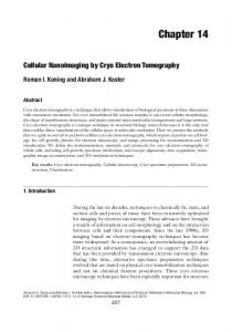
Fluorescence recovery after photobleaching (FRAP) is a powerful, microscopy-based methodology for investigating molecular dynamics within living cells. Whereas traditional fluorescence microscopy yields information in a qualitative “yes or no” manner as to the localisation of molecules in cells, FRAP allows us to elucidate the dynamics of the protein of interest. In order to perform FRAP, the protein of interest must be tagged to a fluorophore. Green fluorescent protein (GFP) is a well-characterised fusion tag widely used for protein labelling in live cells. It was originally discovered in the jellyfish, Aequorea victoria, and has been subsequently modified to produce brighter and more photostable variants (1). In FRAP, fluorescent molecules that localise to a region of interest (ROI) are irreversibly bleached using a high-power laser illumination (see Fig. 1a). The fluorescence recovery over time within the ROI provides details about the dynamics of the protein of interest (2) (see Fig. 1a, b). The rate of fluorescence
*Alex Carisey, Matthew Stroud, and Ricky Tsang contributed equally to the manuscript. Claire M. Wells and Maddy Parsons (eds.), Cell Migration: Developmental Methods and Protocols, Methods in Molecular Biology, vol. 769, DOI 10.1007/978-1-61779-207-6_26, © Springer Science+Business Media, LLC 2011
387
388
A. Carisey et al.
Fig. 1. Principle of FRAP experiment and example. (a) Scheme depicting the photobleaching and fluorescence recovery of a region of interest (ROI) within a focal adhesion (FA) in a cell. Before the bleach event, the fluorescent proteins are uniformly distributed within the structure and are in dynamic equilibrium, immediately after photobleaching, the equilibrium is lost and the fluorescence intensity recovers as fluorescent proteins move back into the ROI. This model represents a reaction-dominant recovery, in which diffusion is negligible. (b) Fluorescence intensity is recorded as a function of time; this enables the half-time of recovery (t1/2), and the mobile and immobile fractions (FM and FI, respectively) to be measured. The fluorescence intensities before and immediately after bleaching are indicated (Finitial and F0, respectively) as well as the intensity after recovery (F∞). (c) Example of a FRAP experiment on a focal adhesion plaque component; FRAP was performed on NIH 3T3 cells transiently expressing vinculin-mEGFP. Panels represent still frames taken at the indicated timepoints (in seconds), throughout the course of the experiment. Dashed circles indicate the bleached ROI, scale bar = 5 mm.
recovery is governed by two major events (3). The first is the diffusion of the fluorescently tagged protein within the localised environment, a fast process occurring over a few milliseconds. The second event is the binding between the fluorescently tagged protein and potential binding partners within the ROI. Most proteins in a cell undergo continuous turnover within complexes allowing bleached fluorescent proteins to be replaced by newly recruited fluorescent proteins, thus leading to the recovery of fluorescence (see Fig. 1a). Such recovery can be quantified by plotting the intensity of the fluorescence over time within the defined ROI, before, during, and after the bleaching event (see Fig. 1b). Further mathematical analysis including curve fitting then allows a detailed assessment of the behaviour of a fluorescently tagged protein within live cells.
26 Fluorescence Recovery After Photobleaching
389
This protocol focusses on FRAP as a method to assess the mobility of fluorescently labelled proteins within focal adhesions of a live cell (see Fig. 1c). We describe here the acquisition of time-lapse images, the bleaching and recovery of fluorescence with an emphasis on the compulsory controls, and cover some aspects of data processing. A complete methodology detailing the processing of raw data from FRAP experiments is described in refs. 4, 5. 1.2. Readouts of FRAP Experiments
Analysis of FRAP experiments yields information about the mobility of the fluorescently tagged protein. Two main parameters can be readily assessed, namely the mobile fraction and the half-time of recovery. The mobile fraction (FM) is the proportion of bleached proteins that are replaced by unbleached proteins during the monitoring of the recovery event. Thus, mobile fraction can be determined by calculating the ratio of fluorescence intensity between the end of the time-lapse recordings (Fµ) and the initial intensity before the bleaching event (Finitial), corrected by the experimental bleach value (F0) (2) (see Fig. 1b). This ratio results in values between 0 and 1, or when expressed as a percentage, between 0% and 100%. Due to binding reactions within the ROI, the theoretical value of 100% of recovery is rarely achieved in practice. Therefore, the recovery reaches a plateau below this value by the end of the time-lapse (see Fig. 1b). Moreover, unintentional bleaching and dynamics of the overall structure during recovery limit the length of the time-lapse recording. In general, proteins that bind strongly to fixed components will have lower mobile fractions than those that interact weakly. Proteins that can freely diffuse show a maximal mobile fraction of 100%, as they do not interact with any partner. The second parameter, the half-time of recovery, is the time that takes for the fluorescence to reach half of its maximal recovery intensity (termed t1/2) (see Fig. 1b). The rate of the recovery depends on the size of the complexes and the stability of the interaction with large or fixed proteins (6). Under some circumstances, the recovery may exceed 100% of the initial fluorescence value. This observation indicates that the bleached structure undergoes a growth phase during the time frame of the experiment. The precise determination of FM and t1/2 is only possible in biological systems that have reached equilibrium before photobleaching so that the total amounts of both fluorescent protein and its binding sites remain constant over the course of the experiment. In this case, the only parameter changing after photobleaching is the equilibrium between the bleached and the unbleached molecules and the return to equilibrium provides the readout of the recovery curve. Finally, reliable measurements will only be obtained for proteins that are part of an immobile complex during the length of the monitored recovery.
390
A. Carisey et al.
1.3. Requirements of the Fluorescent Label
To study the dynamics of a protein in FRAP experiments, the protein of interest must be fused to a fluorophore suitable for expression and monitoring in live cells. To avoid artefacts, this fluorophore should have the following characteristics: 1. It should be bright enough to obtain a high signal-to-noise ratio. 2. It should be photostable to prevent excessive bleaching during time-lapse recordings; however, it should not resist bleaching with the high-power laser. 3. It should not be prone to photoreversible bleaching, an event whereby a proportion of the fluorophore is able to revert back to its original fluorescent state (see Note 1). Such an event can be tested to a certain extent by performing FRAP on fixed cells. 4. It should be monomeric to avoid any irrelevant association between the tagged proteins. The monomeric enhanced GFP (mEGFP) is usually a good choice, since it has all these properties, to a greater extent than the original GFP and many other GFP derivatives. Also most confocal microscopes will be equipped with an argon laser line at 488 nm, which enables high-power photobleaching and low-power monitoring. The use of dyes emitting in the red spectrum is not preferred as bleaching is less efficient with these lasers (see Note 2). Independent of the chosen tag, the fused protein should carry out the same function as the endogenous protein. It is therefore crucial to choose wisely where the fluorescent tag is placed on the protein of interest in order to avoid artefactual readouts (see Note 3).
1.4. Use of the Correct Microscope
FRAP experiments can be carried out on both confocal and widefield microscopes equipped with the necessary laser, but one should be aware of the strengths and weaknesses of the respective systems. Because of their design, wide-field microscopes capture the light emitted by the fluorescent molecules within a thicker optical section of the sample. On one hand, this allows the measurement of low fluorescent intensities that would otherwise be below the threshold for a confocal microscope. Such systems can be fitted with electron multiplying charge-coupled device cameras that have a higher sensitivity, a larger dynamic range, and a faster acquisition rate than most conventional confocal scanning heads. On the other hand, FRAP experiments should be performed on the assumption that the movement of fluorescently labelled proteins is recorded within a focal plane (5). To a certain extent, it is possible to overcome this problem on a wide-field system by the use of background subtraction methods. However, since confocal
26 Fluorescence Recovery After Photobleaching
391
microscopes monitor a precise optical section of a defined thickness, in many cases this type of microscope can deliver more accurate results. In our hands, results of FRAP experiments on adherent cells expressing vinculin-mEGFP (see Fig. 1c) are not significantly different when performed on a Leica SP5 confocal microscope or on a DeltaVision QLM wide-field microscope using the integrated analysis software. 1.5. Validation of Measurements and Data Fitting
When performing FRAP experiments on proteins expressed transiently, the variability of the expression levels of the fluorescent protein can lead to misinterpretation of the results. The level of expression dictates the proportion between the pool of proteins interacting with other molecules and the pool of freely diffusing proteins in the immediate environment. Thus, it is important to determine whether there is a dependence between the FRAP coefficients and the protein expression levels. FRAP coefficients over a wide range of expression levels must be calculated and plotted against the overall cell fluorescence intensity; the slope of the regression line through the data points should not be statistically different from 0, with 95% confidence (see Subheading 3.3.3). Correct data fitting is essential for the interpretation of the results. There are many software packages available but we recommend using MATLAB in order to process large amounts of data. MATLAB allows easy automation of the analysis by fitting the recovery curve and extracting the FRAP coefficients such as FM and t1/2. The fitting parameters depend on several factors, which have been outlined in great detail in ref. 5. Two major processes can influence the kinetics of the recovery: the diffusion of the fluorescently tagged protein and the binding to its partners. Most of the FRAP protocols used by biologists assume that the binding reaction is dominant in their system; however, this should be determined empirically on a protein-by-protein basis. To test whether the binding reaction is dominant, it is important to compare the different fluorescence recovery curves obtained by changing the diameter of the region bleached by the FRAP laser. If the fluorescence recovery curves are similar and give the same rates of recovery independently of the diameter of the bleached spot, then diffusion is negligible. This is referred to as a “reaction-dominant model” (5) in which diffusion occurs a lot faster than the binding reaction. Therefore, the recovery of fluorescence is driven by the following binding equation:
F +S
kon → FS ← koff
392
A. Carisey et al.
where F represents free proteins, S represents unoccupied binding sites for the tagged protein, and FS represents the bound complex. In the case of a single binding state, the predicted FRAP recovery curve is the inverse of an exponential decay. The FRAP data can then be fitted with the following equation to obtain the off-rate constant of binding (koff):
F (t ) = 1 − Ae − koff (t )
The parameter A can be used to calculate the association rate (kon), using: A = kon /(kon + koff ) The mobile fraction is given directly by:
FM = F∞ − F0 /Finitial − F0 The half-time of recovery can be determined from the curve fitting equation with F(t1/2) = (F∞ − F0)/2:
t 1/2 = ln 2/koff
2. Materials 2.1. Cell Culture and Transfection: Equipment and Reagents
1. Laminar flow, tissue culture cabinet. 2. Temperature-regulated, humidified incubator set at 37°C and 5% CO2 gas for the maintenance of mammalian cells. 3. Cell culture medium (Dulbecco’s modified Eagle’s medium, DMEM) supplemented with 10% foetal calf serum (FCS), glutamine, and antibiotics. 4. Trypsin–ethylene diamine tetraacetic acid (EDTA) dissociation solution. 5. Sterile phosphate-buffered saline (PBS) without Mg2+ and Ca2+. 6. Cultured adherent cells (e.g. NIH 3T3 mouse fibroblasts) expressing the protein of interest as a fusion protein with mEGFP (see Note 4). 7. Flasks or Petri dishes treated for cell culture. 8. Six-well tissue culture plates. 9. Transfection kit suitable for the cell type used. We use Lipofectamine Plus reagent (Life Technologies) according to manufacturer’s instructions. 10. mEGFP expression vectors (Clontech).
2.2. Microscope Setup and Reagents for Imaging
The microscope setup described here is currently used in our laboratory; however, any laser scanning confocal microscope with an equivalent setup is suitable.
26 Fluorescence Recovery After Photobleaching
393
1. Leica TCS SP5 AOBS inverted laser scanning confocal microscope (Leica microsystems) (see Notes 5 and 6). 2. Leica HCX PL Apo 63x (lambda blue and NA iris corrected) objective (NA = 1.4) or another high numerical aperture oil immersion objective. 3. An argon 488 nm laser line (see Note 6). 4. Leica LAS AF software for image acquisition and FRAP procedure (supplied with the microscope) or another image acquisition software package. 5. Heated chamber enclosing the microscope stage (see Note 7). 6. Glass bottom sterile culture containers (e.g. glass bottom dishes from MatTek or CellView from Greiner BioOne) for live imaging of cells (see Note 8). 7. Fibronectin from bovine plasma (see Note 9). 8. Ham’s F12 medium supplemented with a final concentration of 25 mM HEPES and pH adjusted to 7.3 using a 1 M NaOH solution. After sterile filtration, supplement with glutamine and antibiotics (see Notes 7 and 10). 9. 4% paraformaldehyde (PFA) solution in PBS (w/v) (see Note 11). 2.3. Software for Analysis
1. Software to extract the fluorescence measurements from the time-lapse images generated by the microscope system. Many software suites controlling microscopes are more or less suitable to perform the complete analysis through simplified wizards (e.g. Leica LAS AF software from Leica Microsystems, softWoRx Suite from Applied Precision). For a better controlled and a more accurate analysis, we prefer to use an opensource image-processing program such as ImageJ (NIH, freely available at http://rsbweb.nih.gov/ij/). 2. Software to perform the data analysis. Any basic spreadsheet software is suitable; however, we recommend the use of a more advanced software package such as MATLAB (The MathWorks), enabling rapid automation in the analysis of large datasets (see Note 12).
3. Methods 3.1. Transfection and Preparation of Cells
This protocol is based on conditions optimised for our measurements of FRAP coefficients of focal adhesion plaque and cytoskeleton-associated proteins. 1. Prepare the mEGFP fusion proteins using standard molecular biology techniques.
394
A. Carisey et al.
2. Transfect cells with construct encoding the fusion protein in a six-well plate using Lipofectamine Plus reagent according to the manufacturer’s instructions (see Note 4). 3. Coat the glass bottom dishes for 1 h at room temperature with 10 mg/mL of fibronectin (see Note 9). 4. After 4 h of incubation, wash the cells twice with sterile PBS. 5. Trypsinize the cells and wash them twice in DMEM supplemented with FCS and plate 5 × 10⁴ cells per 35-mm glass bottom dish (see Note 8). 6. Incubate the cells for 12–48 h in an incubator until the expression of the transfected plasmid reaches its maximum (see Note 13). 7. Replace the DMEM with pre-warmed Ham’s F12 medium (see Note 10). 8. Place the dish in the pre-warmed microscope chamber at least 1 h prior to the FRAP experiment to allow the medium to equilibrate. 3.2. Data Acquisition 3.2.1. Protocol
Three separate phases of the experiment can be distinguished. Firstly, the ROI must be defined and the fluorescence intensity of the GFP fusion protein within this ROI monitored using lowpower laser settings. Secondly, a high-intensity laser pulse is emitted to irradiate the ROI and eliminate the fluorescence within this region. Thirdly, immediately after bleaching, the sample is monitored using the same low-intensity imaging settings as before the bleach. Images are collected at regular time intervals until the intensity in the bleached ROI reaches a plateau. The microscope can be fitted with a real-time autofocusing system to facilitate the acquisition of in-focus images over a long-time period and prevent focus drift due to temperature variations. 1. Select cells expressing a reasonable level of fluorescent protein in the appropriate cellular compartment using the eyepiece of the microscope (see Note 4). 2. Set the parameters following the guidelines provided for monitoring the fluorescence. The individual parameters must be adjusted empirically to obtain high-quality data while achieving three objectives: firstly, obtaining an almost complete bleach in the specified ROI, secondly, monitoring over a sufficient period of time until the fluorescence recovery becomes stable, and finally, keeping the photobleaching and phototoxicity to a minimum (see Note 14). Additionally, the intensity measured must always be confined to the dynamic range of the scan head (see Note 15).
26 Fluorescence Recovery After Photobleaching
395
The settings we use on the confocal microscope are: ●●
●●
●●
●●
●●
●●
●●
●●
●●
Confocal scan head settings: scan rate of 400 Hz for an intermediate image size of 512 × 512 pixels, using bi-directional scanning (see Note 16). Laser power of the 488 nm argon laser line is set to 20% and the transmission of the AOBS to 20% during the monitoring. For the bleaching pulse, the AOBS setting is increased to 100%. Pinhole setting: 1 Airy Unit (see Note 17). Zoom factor: set between 1.6 and 2 to fit the ROI for the bleaching event only. Gain adjustment: 900 V (see Note 18). Offset value: −0.50 (as close to zero as possible until a few zero intensity pixels appears on screen). Beam size (or ROI): set to 1 mm diameter (see Note 19). Iterations: three to five iterations to achieve full bleach (see Note 14). Time-lapse (see Note 20): ●●
●●
One frame every 10 s for three frames before bleach. One frame every 10 s for 10 min after bleach, starting straight after the bleaching event.
3. Adjust precisely the focus and select your desired ROI (see Note 21). 4. Start your time-lapse. 5. Proceed with another cell. Acquire multiple cells showing a broad range of expression levels, as this will give useful information for the analysis (see Subheadings 1.5 and 3.3.3). 3.2.2. Controls
Using this detailed protocol and the same settings as for the experimental samples, several controls must be performed at the same time to accurately interpret the results of a FRAP experiment: 1. Carry out initial experiments to optimise the ideal time course and image acquisition number to ensure that the recovery of fluorescence is complete and photoreversible bleaching is minimised. 2. Bleach several ROI with different spot sizes to test whether diffusion has a major role in the fluorescence recovery. This will allow the user to apply the appropriate mathematical model for determining the protein dynamics according to ref. 5. 3. Ensure that the overall fluorescence intensity of the entire cell is not significantly different before and after photobleaching. Bleached spots must comprise a relatively small proportion of
396
A. Carisey et al.
the cellular pool of fluorescent proteins. To do this, one should perform several FRAP experiments with increasing size and/or number of bleached ROI to determine the limit for the bleach area. Slower recovery curves in experiments with an overall larger bleach area may indicate that recovery of fluorescence is affected by a depletion of the pool of fluorescently labelled proteins. 3.3. FRAP Data Analysis 3.3.1. Intensity Measurements
1. Collect a complete set of FRAP experiments (20–30 cells per condition) and transfer the images to the analysis workstation. 2. Correct any noticeable stage drift by realigning the individual images, e.g. ImageJ plug-in StackReg (7) (see Note 22). 3. Redraw the boundaries of the bleached ROI using the circular selection tool (see Note 19). The ROI position and diameter are likely to be found in the metadata recorded by the microscope software during acquisition. 4. Extract the fluorescence intensity values for: ●●
●●
●●
The bleached ROI. Unbleached areas representative of the background fluorescence. Unbleached structures similar to the bleached target (see Note 23).
5. Label the data in a fully comprehensive manner and store them in a backed-up text file or spreadsheet. 3.3.2. Normalisation and Curve Fitting
Several calculations must be carried out to allow the comparison of the FRAP readouts between different biological samples or FRAP experiments. 1. Plot all the raw data from each ROI separately to validate the integrity of the measurements (see Fig. 2a and Note 24). 2. Obtain the background value (Fbgd[t]) by averaging the fluorescence intensity from unbleached areas representative of the background and subtract this background value from each measurement of a photobleached ROI (Fbleach[t]):
(
)
F [t ] = Fbleach [t ] − Fbgd [t ] 3. Obtain the control value (Fctr[t]) by averaging the fluorescence intensity from several unbleached structures similar to the bleached target (see Note 23) in order to compensate for the overall loss of fluorescence.
26 Fluorescence Recovery After Photobleaching
b
Raw data
3000
bgd1 bgd2 bgd3 ctrl1 ctrl2 FRAP1 FRAP2 FRAP3
2500 2000 1500 1000 500 0
0
100
200
Fractional fluorescence recovery
Fluorescence intensity
a
300
Normalised data FRAP1
1
FRAP2 FRAP3
0.8 0.6 0.4 0.2 0
0
Time
d
Curve fitting 1
FRAP curve Fit
0.8 0.6 F(t) = 1 - A e- koff(t) FM = 66.8902 % t1/2 = 31.9241 sec R = 0.99269
0.4 0.2 0
0
100
100
200
300
Time
200
300
Expression level of the mEGFP fusion protein
Normalised fluorescence intensity
c
397
Correlation
5 4.5 4 3.5 3
4.5:1
2.5 2 1.5 1 0.5
45
50 55 60 65 FM - Mobile fraction (%)
Time
70
Fig. 2. Workflow of analysis of FRAP data. (a) Fluorescence intensities extracted from the time-lapse images are individually plotted over time to visualise any abnormal behaviour. The intensities recorded within several bleached ROI are termed FRAP1, FRAP2, and FRAP3. The background readings are termed bgd1, bgd2, and bgd3; and finally, the recordings for the unintentional bleaching are labelled as ctrl1 and ctrl2. (b) After background subtraction and correction for the postbleach intensity, the fractional fluorescence recovery of the three bleached ROI are plotted over time. The intensity of the monitored fluorescence now varies between 1 (prebleached value) and 0 (immediately after the bleach event). (c) Multiple fractional fluorescence recovery curves acquired in the same cell are averaged and plotted with their standard deviation of the mean. The curve is the best fit obtained from the experimental data. The main parameters discussed in the text have been extracted for these data. (d) A scatter plot is shown here to illustrate the absence of correlation between the overall fluorescence intensity of the cell, e.g. the expression level of the tagged protein, and the mobile fraction over a 4.5-fold range. A similar graph should be plotted with the half-time of recovery and the overall fluorescence intensity (see Subheading 3.3.3).
4. Correct each measurement with the background-subtracted control value from an unbleached ROI to obtain the experimental recovery (Rnorm[t]) as follows:
(
)
Rnorm [t ] = F [t ]/ Fctr [t ] − Fbgd [t ] 5. Correct the experimental recovery with the first postbleach fluorescence intensity set to zero (F0) to obtain the fractional recovery measurement (Rfrac[t]):
Rfrac [t ] = (Rnorm [t ] − F0 )/(1 − F0 ) 6. Average the multiple Rfrac[t] obtained within the same cell and over the same time course.
398
A. Carisey et al.
7. Plot the average fractional fluorescence recovery curve (Rfrac[t]) obtained (see Fig. 2b). 8. Superimpose multiple fractional fluorescence recovery curves obtained from different cells and use them to calculate the standard deviation (see Fig. 2c). 9. The mobile fraction and the half-time of recovery can already be estimated from this curve, but a more accurate approach requires curve fitting. 10. Export the data to MATLAB. 11. Fit the plotted data (see Fig. 2c) using the following equation with the ezyfit toolbox for MATLAB (see Note 25):
F (t ) = 1 − Ae − koff (t ) 12. Obtain the FRAP coefficients.
3.3.3. Evaluation of the Relationship Between Expression Level and FRAP Coefficients
To assess any relationship between the expression level of the fluorescently tagged protein and the FRAP coefficients which could invalidate the results, a correlation study must be performed: 1. With the help of the selection tool in ImageJ, measure the intensity of the fluorescence in the cell before the bleaching event. 2. Plot the overall intensity value against its estimated mobile fraction in a scatter plot (see Fig. 2d); in a second figure, plot the same value against the estimated half-time of recovery. 3. Calculate the slope of the regression line through the data points. It must not be statistically different from 0 at 95% confidence.
4. Notes 1. Photoreversible bleaching can pose a problem during the quantitative analysis of FRAP data and lead to an artefactual measurement of protein dynamics. Furthermore, different fluorescent proteins show different rates of photoreversible bleaching; therefore, comparisons between GFP variants within an experiment may give misleading results. Photoreversible bleaching can occur in the GFP species on a millisecond time scale (8). It is known that YFP species also exhibit photoreversible bleaching, which occurs in the timescale of seconds and is dependent on complex protonation reactions (9). The longer time scale associated with YFP may become apparent in experiments with short time intervals, therefore GFP is usually the preferred option.
26 Fluorescence Recovery After Photobleaching
399
2. Being able to completely bleach the fluorescence emitted by the tagged protein is crucial. Theoretically, bleaching using a high-power laser beam can be achieved on any fluorescent protein, depending on the availability of the appropriate laser line on the microscope system; this should match the excitation peak of the targeted molecule. For example, the red fluorescent protein (RFP) or its more photostable equivalent mCherry (10) may be used for FRAP; however, the fluorescence quantum yield is significantly lower than that of EGFP. Also, suitable lasers (such as the Helium-Neon Orange 594 nm) are known to be weak and may not achieve full bleach, therefore the GFP variant is preferred. 3. Ideally, the fluorescent tag should be inserted in at least two independent positions, for example on the N- or C-terminus end of the protein. The localisation of the overexpressed construct should be similar to that of the endogenous protein, and issues about a potential perturbation of function must be considered if the FRAP coefficients obtained are significantly different between the two constructs. 4. In most cases, either transient or stable expression of the fusion protein in cells can be performed. Using a stable cell line for FRAP ensures that the measurements are more consistent by reducing the variability of expression levels (see also Subheading 3.3.3). 5. The Acousto-Optical Beam Splitter (AOBS) is a common feature on more recent confocal microscopes allowing the physical separation of emission and excitation light paths with high transmission efficiency. An Acousto-Optical Tunable Filter (AOTF) allows the rapid alternation between the lasers and the adjustment of their repective intensities by modifying the transmission coefficient, as opposed to changing the power of the laser emission itself. This component is essential to perform automated monitoring and reduce bleaching of the sample during the recovery period. 6. The use of laser-based microscopes is restricted to persons who have been adequately trained and are familiar with the local safety regulations. 7. We use a temperature- and CO2-controlled chamber to provide the optimal conditions for live imaging. It is possible to avoid the need for CO2 by using a CO2-independent buffered system such as HEPES. 8. Plastic culture dishes and plates are poorly suited for fluorescence studies as they exhibit non-stable auto fluorescence (11), therefore cells must be transferred to a glass bottom dish after transfection.
400
A. Carisey et al.
9. Other extracellular matrix proteins such as laminin, vitronectin, or collagen may be required to ensure the spreading of some cell lines. 10. In order to reduce background fluorescence due to the presence of riboflavin and phenol red in DMEM, Ham’s F12 medium is preferred. Riboflavin exhibits high autofluorescence in the excitation range of 450–490 nm and emission range of 500–560 nm. Phenol red has a maximum excitation peak around 555 nm. To further minimise the autofluorescence, FRAP experiments are preferably performed in lowserum or serum-free medium. 11. PFA is a toxic powder that must be handled with care using gloves and a respiratory mask in an isolated environment. A 4% PFA solution in PBS (w/v) will dissolve overnight with constant stirring at 50°C. The stock solution can be aliquoted and stored at −80°C for a year. Thawed aliquots must be kept at 4°C and used within a week. Fixation of cells is performed at room temperature for 15 min followed by three washes in PBS. 12. MATLAB can be linked to ImageJ through an additional Java package created by Daniel Sage and Dimiter Prodanov (Biomedical Imaging Group, Swiss Federal Institute of Technology, Lausanne, Switzerland, http://bigwww.epfl.ch/ sage/soft/mij/). 13. The expression of the construct in a suitable cell line for the study must be monitored by fixing the cells in PFA at various time points after transfection as the expression level and maturation speed of the fluorescently tagged protein vary considerably depending on the tag and the cell line. Moreover, the delivery of the overexpressed protein in the appropriate cellular compartment is another feature that varies, as it is dependant on the renewal rate of the endogenous protein. 14. Despite the fact that the parameters will be used to monitor living cells, it is more convenient to optimise the settings using a fixed sample maintained in the same conditions as for the live cells. The laser settings for the bleaching event should be set to achieve a sufficient decrease in fluorescence within the ROI. As a guideline, we consider that the first reading after bleach should be less than 20% of the measurement before the bleaching event. Although this value is subject to discussion as the bleaching illumination must be kept as low as possible, for the following two reasons: firstly, to avoid excessive phototoxicity and secondly, because the beginning of fluorescence recovery must not overlap with the last bleaching iteration. Indeed, the bleaching duration must be confined to a limited space (i.e. the ROI) and time (ideally instantaneous) to allow accurate measurement. Unfortunately,
26 Fluorescence Recovery After Photobleaching
401
there is no general rule and it is more a case of trial and error for the user to obtain the optimal bleaching and imaging parameters. 15. It is crucial to adjust the acquisition parameters of the photomultiplier tube (PMT) in order to remain in the dynamic range of intensity acquisition. Saturation of fluorescence intensity during the time-lapse will result in inaccurate measurements of FRAP coefficients. 16. On the majority of line scanning confocal microscopes, an option is available for bi-directional scanning; however, the user must bear in mind that phase correction may need to be adjusted. This allows the scan head to image the sample in both directions along the x-axis and inevitably increase the acquisition rate. Additionally, the frame averaging function should be avoided while doing live measurements as it leads to a loss of time resolution. 17. The pinhole value, determined by the numerical aperture of the objective and the light wavelength, should ideally be adjustable. For live cell work, the pinhole should be opened wide enough to acquire an adequate signal, while keeping the laser intensity low to minimise photobleaching and phototoxicity. Meanwhile, opening the pinhole affects the resolution by increasing the thickness of the optical section. 18. The PMT gain value should be around 900 V. A value below 600 V means that the laser line intensity can be lowered; conversely, it needs to be increased if the gain setting is above 1,100 V. 19. If these experiments will be analysed according to the method detailed by Sprague et al. (5), the ROI must be circular. 20. It is necessary to record three to five frames before the bleaching step to obtain the value of the initial maximum intensity within the ROI. 21. It is recommended to bleach multiple ROI of identical size for each time-lapse. Recovery curves obtained from multiple ROI within the same cell should be averaged after normalisation to obtain smooth data (see Subheading 3.3.2 and Fig. 2c). Pooling data is acceptable under these circumstances as the level of expressed fusion proteins (i.e. both fractions of bound and free molecules) is the same between the different ROI. 22. Plug-in created by Philippe Thévenaz (Biomedical Imaging Group, Swiss Federal Institute of Technology, Lausanne, Switzerland, http://bigwww.epfl.ch/thevenaz/stackreg/). 23. The data have to be corrected for unintentional bleaching that occurs during the monitoring phases. Two techniques can be used: the first consists of recording the fluorescence
402
A. Carisey et al.
intensity within several identical unbleached regions to the one displayed in the same cell as the bleached ROI. The second technique involves the recording of the averaged intensity of the cell. 24. Discard any sets of data that exhibit any of the following defects: inconsistent background fluorescence intensities, unstable prebleach intensities, and recovery curves that do not exhibit a plateau. 25. Ezyfit toolbox for MATLAB created by Frederic Moisy (Laboratory FAST, University Paris Sud, Paris, France, http://www.fast.u-psud.fr/ezyfit/).
Acknowledgments We would like to thank Dr. Janet Askari for critical reading of the manuscript. CB acknowledges BBSRC (BB/G004552/1). The Bioimaging Facility microscopes used in this study were purchased with grants from BBSRC, Wellcome Trust and the University of Manchester Strategic Fund. References 1. Tsien, R. Y. (1998) The green fluorescent protein, Annu Rev Biochem 67, 509–544. 2. Axelrod, D., Koppel, D. E., Schlessinger, J., Elson, E., and Webb, W. W. (1976) Mobility measurement by analysis of fluorescence photobleaching recovery kinetics, Biophys J 16, 1055–1069. 3. Sprague, B. L., and McNally, J. G. (2005) FRAP analysis of binding: proper and fitting, Trends Cell Biol 15, 84–91. 4. Sprague, B. L., Muller, F., Pego, R. L., Bungay, P. M., Stavreva, D. A., and McNally, J. G. (2006) Analysis of binding at a single spatially localized cluster of binding sites by fluorescence recovery after photobleaching, Biophys J 91, 1169–1191. 5. Sprague, B. L., Pego, R. L., Stavreva, D. A., and McNally, J. G. (2004) Analysis of binding reactions by fluorescence recovery after photobleaching, Biophys J 86, 3473–3495. 6. Lippincott-Schwartz, J., Snapp, E., and Kenworthy, A. (2001) Studying protein dynamicsin living cells, Nat Rev Mol Cell Biol 2, 444–456. 7. Thevenaz, P., Ruttimann, U. E., and Unser, M. (1998) A pyramid approach to subpixel
r egistration based on intensity, IEEE Trans Image Process 7, 27–41. 8. Dickson, R. M., Cubitt, A. B., Tsien, R. Y., and Moerner, W. E. (1997) On/off blinking and switching behaviour of single molecules of green fluorescent protein, Nature 388, 355–358. 9. McAnaney, T. B., Zeng, W., Doe, C. F., Bhanji, N., Wakelin, S., Pearson, D. S., Abbyad, P., Shi, X., Boxer, S. G., and Bagshaw, C. R. (2005) Protonation, photobleaching, and photoactivation of yellow fluorescent protein (YFP 10 C): a unifying mechanism, Biochemistry 44, 5510–5524. 10. Shaner, N. C., Campbell, R. E., Steinbach, P. A., Giepmans, B. N. G., Palmer, A. E., and Tsien, R. Y. (2004) Improved monomeric red, orange and yellow fluorescent proteins derived from Discosoma sp. red fluorescent protein, Nat Biotechnol 22, 1567–1572. 11. Piruska, A., Nikcevic, I., Lee, S. H., Ahn, C., Heineman, W. R., Limbach, P. A., and Seliskar, C. J. (2005) The autofluorescence of plastic materials and chips measured under laser irradiation, Lab Chip 5, 1348–1354.