electrons naturally corresponds to charge transport and eventually to the ...... the energy gap between the HOMO and the LUMO levels to be A0, i.e., we have ...... called disconnected diagrams, as they are composed of two different diagrams.
- -
Riku Tuovinen
J ¨ ¨ F Pro gradu -tutkielma Ohjaaja: Robert van Leeuwen 23. helmikuuta 2011
ii
Abstract In this master’s thesis microscopical systems of molecules and atomic chains are studied to obtain information about quantum-transport phenomena. Both exact diagonalization method through second quantization and perturbation theory approach with Feynman diagrams are described, and then the energy spectra for the studied systems are calculated using the two methods. The essential part of the method of exact diagonalization is simply to consider different quantum configurations of the studied system. After this the Hamiltonian matrix is constructed from all the possible states, and finally solving the actual problem is finding the eigenvalues and eigenvectors of this matrix. Only problem is, when the studied systems are large, that the dimension of the Hamiltonian matrix grows rapidly leading the diagonalization being quite a demanding task (even with powerful computers). For the perturbation-theory approach, on the other hand, lots of preparations are needed before any results arise. These preparations include a wide background information about Green’s functions, equations of motions, not forgetting the perturbative expansion with Feynman diagrams. Once ready and prepared, the non-interacting Green’s functions for the studied systems can be constructed, after which the self-energy calculations with Feynman rules can be done. From the self-energy the total Green’s function for the interacting system can be derived, and ultimately from the total Green’s function all the essential physical properties of the studied systems are obtained. The studied system includes a two-site molecule and an N-site tight-binding chain with interactions between the molecule and the chain. The main focus involves adding and removing particles to the molecule, and then studying the response of the chain next to the molecule. In this kind of study the so-called image-charge effect arises when the added or removed particle on the molecule affects the electron density on the terminal site of the chain. The actual findings of the thesis are limited to comparing the results obtained from perturbation theory to the exact ones. It is seen clearly that the perturbation theory in first order (Hartree–Fock) does not take into account the interactions of the studied system, but already the second-order calculations converge almost to the exact result.
Contents 1
Introduction
2
Many-particle problem in terms of quantum field theory 2.1 Second quantization . . . . . . . . . . . . . . . . . . . 2.1.1 Occupation number representation . . . . . . . 2.1.2 Creation and annihilation operators . . . . . . 2.1.3 Field operators and time-evolution . . . . . . . 2.1.4 Hubbard model . . . . . . . . . . . . . . . . . . 2.1.5 Tight-binding approximation . . . . . . . . . . 2.2 Propagators . . . . . . . . . . . . . . . . . . . . . . . . 2.3 Vacuum amplitude . . . . . . . . . . . . . . . . . . . .
3
4
5
5
Many-particle perturbation theory 3.1 Green’s functions and statistical physics 3.2 Time evolution and equations of motion 3.3 Perturbative expansion . . . . . . . . . . 3.4 Dyson equation . . . . . . . . . . . . . . 3.5 Feynman rules . . . . . . . . . . . . . . . Mathematical tools 4.1 Complex contour integrals . . . . . . 4.1.1 Cauchy’s integral theorem . . 4.1.2 Cauchy’s integral formula . . 4.1.3 Important improper integrals 4.1.4 Cauchy’s principal value . . 4.2 Integral transforms . . . . . . . . . . 4.2.1 Fourier transform . . . . . . . 4.2.2 Hilbert transform . . . . . . .
. . . . . . . .
. . . . . . . .
. . . . .
. . . . . . . .
. . . . .
. . . . . . . .
. . . . .
. . . . . . . .
. . . . .
. . . . . . . .
. . . . .
. . . . . . . .
. . . . .
. . . . . . . .
. . . . .
. . . . . . . .
. . . . .
. . . . . . . .
. . . . . . . .
. . . . .
. . . . . . . .
Model system: molecule and chain 5.1 Preliminaries . . . . . . . . . . . . . . . . . . . . . . . . . 5.2 Solving the eigenvalue problem . . . . . . . . . . . . . . 5.2.1 Tight-binding chain . . . . . . . . . . . . . . . . 5.2.2 Two-site molecule . . . . . . . . . . . . . . . . . 5.2.3 Interaction between the molecule and the chain iii
. . . . . . . .
. . . . .
. . . . . . . .
. . . . .
. . . . . . . .
. . . . .
. . . . . . . .
. . . . .
. . . . . . . .
. . . . .
. . . . . . . .
. . . . .
. . . . . . . .
. . . . .
. . . . . . . .
. . . . .
. . . . . . . .
. . . . .
. . . . . . . .
. . . . .
. . . . . . . .
. . . . .
. . . . . . . .
. . . . .
. . . . . . . .
. . . . .
. . . . . . . .
. . . . .
. . . . . . . .
. . . . .
. . . . . . . .
. . . . .
. . . . . . . .
. . . . .
. . . . . . . .
. . . . .
. . . . . . . .
. . . . .
. . . . . . . .
. . . . .
. . . . . . . .
. . . . .
. . . . . . . .
. . . . .
. . . . . . . .
. . . . .
. . . . . . . .
. . . . .
. . . . . . . .
. . . . .
. . . . . . . .
. . . . .
. . . . . . . .
. . . . .
. . . . . . . .
. . . . .
. . . . . . . .
7 7 8 9 18 20 21 22 24
. . . . .
27 27 31 38 42 44
. . . . . . . .
47 47 47 51 52 54 55 55 56
. . . . .
57 57 58 58 63 65
Contents
iv
5.3
5.4 5.5
Solution via perturbative expansion . . . . . . . . . . . . 5.3.1 Non-interacting Green’s function for the molecule 5.3.2 Non-interacting Green’s function for the TB chain 5.3.3 Hamiltonian and interactions . . . . . . . . . . . . 5.3.4 Two-site molecule and two-site TB chain . . . . . 5.3.5 Self-energy calculations . . . . . . . . . . . . . . . Infinitely long chain . . . . . . . . . . . . . . . . . . . . . . Computational methods . . . . . . . . . . . . . . . . . . . 5.5.1 Exact diagonalization . . . . . . . . . . . . . . . . 5.5.2 Numerical integrations for the infinite chain . . .
. . . . . . . . . .
. . . . . . . . . .
. . . . . . . . . .
. . . . . . . . . .
. . . . . . . . . .
. . . . . . . . . .
. . . . . . . . . .
. . . . . . . . . .
. . . . . . . . . .
. . . . . . . . . .
. . . . . . . . . .
. . . . . . . . . .
. . . . . . . . . .
. . . . . . . . . .
69 69 71 73 74 75 81 86 86 87
6
Discussion 89 6.1 Molecule and truncated chain . . . . . . . . . . . . . . . . . . . . . . . . . . . . . . 89 6.2 Infinitely long chain . . . . . . . . . . . . . . . . . . . . . . . . . . . . . . . . . . . . 91
7
Conclusion
93
List of symbols Aˆ (H)
Operator in Schrodinger (Heisenberg) picture ¨
Aˆ (†)
General annihilation (creation) operator
G(N) (1, . . . , N; N0 , . . . , 10 )
N-particle propagator, i.e., Green’s function from (x0i , t0i ) to (xi , ti )
ϕn (x)
One-particle orbitals
ψ(x)
Single-particle wavefunction (in one dimension)
Ψ(x1 , . . . , xN )
Many-particle wavefunction
ψˆ (†) (x)
Field operator for annihilating (creating) particle from (to) x
Σ
Self-energy
T(C)
Time (contour) ordering operator
ˆ (t, t0 ) U
Time-evolution operator from t0 to t
x
Collective vector for position vector r and spin index σ: x = (r, σ)
Z
Partition function
Conventions • Vectors are expressed with bold-face letters, matrices have indices as subscripts. • Operators are marked with a hat ˆ . • In numerical calculations we use units: h¯ = me = e = (4π�0 )−1 = 1 .
Chapter 1
Introduction Quantum theory is (so far) the most accurate representation of the Nature at the microscopic level. The theory has been applied succesfully to different phenomena of matter and energy, which can differ considerably in the order of magnitude. This so-called standard model of particle physics covers the research fields from elementary particles, to many-particle materials science, and even further to neutron stars and to other astrophysical objects in cosmological scale. Apart from these the most everyday interaction – gravity – remains an open problem in fundamental quantum theory. At first quantum physics concerned the movement of particles as mechanical objects leaving, e.g., the electromagnetic interaction completely to Maxwell’s era. Because of this the name quantum mechanics has remained to describe many phenomena at the microscopic level. The elementary quantum mechanics was developed mainly by Heisenberg, Schrodinger and Dirac ¨ during the years 1925–1926 [15, 27, 6]. It did not, however, take very long time until also the electromagnetic field was quantized and soon after this also the material fields for fermions and bosons. These theories combined to quantum electrodynamics (QED) and quantum field theory (QFT). The original single-particle quantum mechanics is often called first quantization, whereas the quantum-field theoretical description is called second quantization. In this project we aim to study electron dynamics in many-particle systems. The motion of electrons naturally corresponds to charge transport and eventually to the quantity known as current. Microscopical devices can already be constructed and they can be utilized in, e.g., nanotechnology and molecular electronics. Namely solid–molecule interfaces are typical components, but the actual quantum-level physics in the background of these applications is known quite restrictedly. The theoretical models rely mostly on density functional theory which emanates from single-particle quantum mechanics. Obtaining results from these theoretical models can be quite a tedious task when considering the numerical methods. Many-particle perturbation theory provides another method to study the interesting model systems corresponding to, e.g., nanoscale electronics chips. Computationally speaking the many-particle perturbation theory might not be any more profitable method than the ones with density functional theory, but the idea of capturing the essential physics from studied system through a collection of Feynman diagrams is (at least intuitively) advantageous. More explicitly, in many-particle perturbation theory the system is first assumed to be non-interacting. Then the interactions (due to Coulomb force or tunneling for instance) are assumed to be small enough that they can be interpreted perturbatively. The terms of the perturbation series are then described as symbolic diagrams for which certain 5
6
Chapter 1. Introduction
calculation rules arise. The outline of this thesis is as follows. After this short introduction we present a theoretical background by stating the many-particle problem in terms of quantum field theory. After this a little more background information about many-particle perturbation theory is described, after which it follows a short introduction to complex analysis because of the needed mathematical methods. Then the present study is described and analyzed in detail with the help of the stated background theory. After the actual calculations we present the results and discuss them thoroughly. The last chapter contains a conclusion and an outlook for future considerations.
Chapter 2
Many-particle problem in terms of quantum field theory In this chapter we will set the basis for the field of study. The framework we will be working is the quantum field theory, and for for the many-particle phenomena we introduce essential parts of this particular theory. We will be following the representation of Refs. [20, 24, 28, 33] and the lecture notes of a course in many-particle quantum mechanics by Robert van Leeuwen.
2.1
Second quantization
The formalism of second quantization is a quantum field theoretical representation of manyparticle systems. This formalism is especially necessary when we are dealing with systems in which the number of particles is itself variable. Originally, second quantization was developed for the study of photons in radiation theory by P. Dirac in 1927 [7]. The method was later extended to bosons (by P. Jordan and O. Klein) in 1927 and to fermions (by P. Jordan and E. Wigner) in 1928 [17, 32]. Usually, the elementary quantum mechanics is formulated via first quantization, i.e., the normal ˆ which in turn observables for position x and momentum p are replaced by operators xˆ and p, obey the so-called canonical commutation relation [xˆ , pˆ ] = i¯h. However, in second quantization we quantize the wave function itself by replacing the complex-valued function ψ(x) by an operator ψˆ (x). The terminology here can be rather misleading since first quantization refers to the quantization of a single-particle system while second quantization refers to the quantization of a many-particle system, but both systems are being quantized only once and separately. Quantum mechanics of an N-particle system is strongly based on the wave function Ψ (x1 , . . . , xN ), where both the position ri and the spin projection σi of the i:th particle are included in the coordinate xi . When studying indentical particles, their exchange must not change any physical quantities, i.e., � � � � Ψ x1 , . . . , xi , . . . , x j , . . . , xN = eiθ Ψ x1 , . . . , x j , . . . , xi , . . . , xN , (2.1) where eiθ is a phase factor. Interchanging any pair (i, j) of particles twice should amount to no interchange, hence, (eiθ )2 = 1 gives eiθ = ±1. This (anti)symmetry of the wave function 7
Chapter 2. Many-particle problem in terms of quantum field theory
8
for (fermions) bosons is called Spin-statistics theorem [25]. This theorem follows from the assumptions of 1) Lorentz invariance, 2) causality and 3) unitarity. It should, however, be noted that the theorem holds only in three spatial dimensions (and above) because in one and two dimensions the exchange of particles is more restricted, as there must be some plane where the particles are rotating (2D) or a line where the particles are colliding with each other (1D). Next thing to consider is, what kind of basis we need to construct for the general wave function in Eq. (2.1). When studying N identical fermions1 we need to have a fully antisymmetrized wave function. Although it is possible to expand the total wave function in an orthonormal basis {ϕn (x)} [with ϕn (x) = hx|ϕn i being a projection on the position-spin eigenbra hx| = hrσ| of the basis ket |ϕn i], the antisymmetry property makes calculations somewhat difficult. The N-particle basis function, with respect to the expansion is to be done, is a sum of all different permutations of one-particle basis functions X sgn(P)ϕn1 (xP(1) )ϕn2 (xP(2) ) · · · ϕnN (xP(N) ) , (2.2) P
where P refers to permutations of 1, 2, . . . , N. The sign of the permutation sgn(P) is either plus for even permutations or minus for odd permutations. The sum in Eq. (2.2) contains N! terms, and it easy to imagine how convoluted, e.g., actions of certain operators become when we express the basis functions as projections on the normalized position-spin eigenbra of the corresponding normalized basis ket 1 X 1 X √ (2.3) sgn(P)hxP(N) | · · · hxP(2) |hxP(1) | √ sgn(P)|ϕnP(1) i|ϕnP(2) i · · · |ϕnP(N) i . N! P N! P Fortunately, the formalism of second quantization gives us a shortcut for the stated headache above, as the expressions become more compact. It turns out that there are certain operators which have all the symmetry properties of the system built into them. One remarkable thing to mention before tackling the formal development of the occupation number representation in detail, is the idea by V. Fock from 1932 [12]. He showed a one-to-one correspondence between wave-function description and occupation number representation, and introduced the so-called Fock space. If we consider the number of particles as an observable capable of assuming various values (N = 0, 1, 2, . . .), we have one Hilbert space corresponding to the one-particle system, a different Hilbert space for the two-particle system and so on. The Fock space is a collection of all these Hilbert spaces with different number of particles. In fact, the Fock space is a direct sum of i-particle Hilbert spaces F =
N M
Hi ,
(2.4)
i=0
where also the zero-particle Hilbert space is included, which is simply an empty, one-dimensional space.
2.1.1
Occupation number representation
We notice that the form of the basis functions in Eq. (2.2) is the definition of a determinant. The fully antisymmetrized wave function can therefore be represented as a so-called Slater 1 In
this thesis we will be considering fermions only.
2.1. Second quantization
determinant
9
ϕn (x1 ) . . . ϕn (xN ) 1 1 1 .. .. . . . Ψ (x1 , . . . , xN ) = √ . . . N! ϕnN (x1 ) . . . ϕnN (xN )
(2.5)
As said earlier, the determinant expression is a bit clumsy to carry around, and because of this, we adopt a compact way of writing the wave function in Eq. (2.5) by noticing that the particles are indistinguishable: The essential information then is, how many particles there are in a single-particle state. We can then equally well specify the non-interacting state as (without normalization) Ψ (x1 , . . . , xN ) = hxN , . . . , x1 |n1 , . . . , nN i , (2.6) meaning, that there is n1 particles in state ϕn1 and nN particles in state ϕnN , with ni being either 1 or 0 because of the Pauli’s exclusion principle. The form of the wave function in Eq. (2.6) is called the occupation number representation. It is also important to note that the states in occupation number representation form a complete orthonormal set of basis functions (just as the original Slater determinants do), i.e., we have hn0N , . . . , n01 |n1 , . . . , nN i = δn01 ,n1 . . . δn0N ,nN , and
X
|n1 , . . . , nN ihnN , . . . , n1 | = 1 .
(2.7) (2.8)
n1 ,...,nN
The particle number operator is easily accessible in occupation number representation. When we act with a number operator to a state, we get exactly the number of particles in that particular state nˆ i |n1 , . . . , ni , . . . , nN i = ni |n1 , . . . , ni , . . . , nN i , (2.9) and the total number of particles N in a system is then given simply by X ˆ 1 , . . . , nN i = N|n ni |n1 , . . . , nN i .
(2.10)
i
2.1.2
Creation and annihilation operators
We can look into the occupation number representation more precisely by introducing so-called creation and annihilation operators. These operators map the space of N-particle states to spaces with N ± 1-particle states, i.e., add or remove particles. For the consideration here, we follow the representation given in [28]. Due to the Pauli’s exclusion principle, two identical fermions must not occupy the same state. When we consider adding particles, i.e., acting to a state with creation operators, we must pay attention to the fermion statistics: applying them twice should amount to zero. Consider now an N-particle state |n1 , n2 , . . . , nN i = aˆ†1 , aˆ†2 , . . . , aˆ†N |0i , (2.11) where the operators aˆ† are creation operators acting to a vacuum state |0i. If we interchange first two occupancies we get the same state except for the sign (antisymmetricity) |n2 , n1 , . . . , nN i = −aˆ†2 , aˆ†1 , . . . , aˆ†N |0i .
(2.12)
Chapter 2. Many-particle problem in terms of quantum field theory
10
n o We then realize that aˆ†1 aˆ†2 = −aˆ†2 aˆ†1 , i.e., the operators anticommute: aˆ†1 , aˆ†2 = 0. Naturally, this generalizes to any two creation operators in Eq. (2.11) and we have n o aˆ†i , aˆ†j = 0 . (2.13) The impossibility of double occupation2 is naturally included in Eq. (2.13). By fermionic nature of particles we can now rewrite our N-particle state in Eq. (2.11) as � �n1 � �n2 � �nN aˆ†2 . . . aˆ†N |n1 , n2 , . . . , nN i = aˆ†1 |0i , (2.14) with ni ∈ {0, 1}. If we then consider the addition of a particle into state i we have aˆ†i | . . . , ni , . . .i = (1 − n1 )(−1)
P
j 0), the integration contour can be closed by a semicircle in the UHP for λ > 0, and in the LHP for λ < 0. Then Z (4.23) lim eiλz f (z)dz = 0 . ρ→∞
Cρ : |z|=ρ
This result in Eq. (4.23) is called Jordan’s lemma. Notice that on the semicircle Cρ , where (in polar form) z = ρeiθ = ρ (cos θ + i sin θ), we have eiλz = eiλρ(cos θ+i sin θ) = eiλρ cos θ−λρ sin θ i h � � �� iλρ� cos θ−λρ sin θ � θ−λρ sin θ 1/2 �cos = e� e−iλρ i1/2 h = e−2λρ sin θ
= e−λρ sin θ .
(4.24)
If λ > 0 and sin θ ≥ 0, then e−λρ sin θ → 0 as ρ → ∞ in the UHP for which 0 ≤ θ ≤ π. On the other hand, if λ < 0 we must have sin θ ≤ 0, which is what happens when π ≤ θ ≤ 2π, i.e., in the LHP. Thus, when we convert integrals, such as in Eq. (4.22), into closed-contour integrals (in order to use Cauchy’s integral formula), the poles need to be considered only in either half of the complex plane.
4.1.4
Cauchy’s principal value
We consider an improper integral Z
b
f (x)dx
(4.25)
a
with the function f (x) having a singular point x0 ∈ [a, b], i.e., lim f (x) = ∞ .
(4.26)
x→x0
If the function is integrable over every portion of the interval [a, b] without the point x0 then we define Z Z Z b
x0 −δ
f (x)dx = lim
δ→0
a
b
f (x)dx + lim �→0
a
x0 + �
f (x)dx ,
(4.27)
when the limit exists as δ and � tend to zero independently. Otherwise the integral is said to diverge. However, if we have δ = �, we define the integral in Eq. (4.27) as the Cauchy’s principal value (“valeur principale”) Z x −δ Z b Z b 0 f (x)dx . (4.28) lim f (x)dx + f (x)dx C VP δ→0
a
x0 + δ
a
4.2. Integral transforms
55
This means that if the integral as such diverges, but the principal value exists, the integral is defined as its principal value. And how exactly does the principal value defined above relate to complex integrals studied in this section? In the next chapter we will study the following type of integral Z ∞ g(x)dx . (4.29) lim η→0 −∞ x − a ± iη We may rewrite the integrand without the function g(x) as follows 1 x − a ± iη
x − a ∓ iη (x − a ± iη)(x − a ∓ iη) x−a∓η 2 x − xa ∓ xiη − xa + a2 ± aiη ± xiη ∓ aiη + η2 x − a ∓ iη 2 x − 2xa + a2 + η2 η x−a ∓ i . (x − a)2 + η2 (x − a)2 + η2
= = = =
We also introduce a form of the deltafunction " # η 1 δ(x − a) = lim . η→0 π (x − a)2 + η2 Then we get back to the integral in Eq. (4.29) and obtain # Z ∞" Z ∞ g(x)dx η x−a = lim lim ∓i g(x)dx η→0 −∞ x − a ± iη η→0 −∞ (x − a)2 + η2 (x − a)2 + η2 Z ∞ Z ∞ g(x)dx ∓ iπ δ(x − a) g(x)dx = VP −∞ −∞ x − a Z ∞ g(x)dx = VP ∓ iπg(a) . −∞ x − a
4.2
(4.30)
(4.31)
(4.32)
Integral transforms
This section is a very brief one as we only state the definitions for the used methods within the field of integral transforms.
4.2.1
Fourier transform
For f ∈ S(Rn ), where S(Rn ) is an n-dimensional Schwartz space, the Fourier transform is a bijection F : S(Rn ) → S(Rn ) with Z 1 F [ f (x)] = dx e−ip·x f (x) , (4.33) n/2 n (2π) R and the inverse transform is F
−1
1 [ f (p)] = (2π)n/2
Z Rn
dp eip·x f (p) .
(4.34)
Chapter 4. Mathematical tools
56
4.2.2
Hilbert transform
The Hilbert transform of a real function f (t) is defined as a convolution with the function h(t − τ) = [π(t − τ)]−1 Z ∞ f (τ) 1 dτ . (4.35) H [ f (t)] = VP π t −τ −∞ Because of the possible singularity at τ = t, the integral is considered as a Cauchy’s principal value integral, introduced in the previous section.
Chapter 5
Model system: molecule and chain In this chapter, we consider a physical model that can be studied by using the formalism introduced in Chaps. 2 and 3.
5.1
Preliminaries
Consider a model with a two-site molecule and an N-site tight-binding (TB) chain. The Hamiltonian describing the model system is constructed from three different parts, viz. Hˆ tot = Hˆ ch + Hˆ mol + Vˆ ,
(5.1)
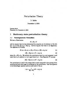
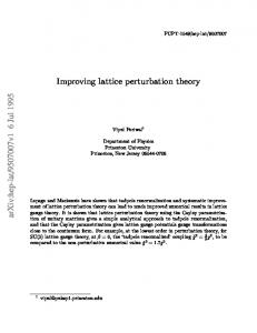
where Hˆ ch is the TB Hamiltonian for the chain, Hˆ mol is the Hamiltonian for the molecule, and the operator Vˆ stands for the interaction between the molecule and the terminal (1st) site of the chain. The interacting electrons of the molecule are allowed to be located either on the lowest unoccupied molecular orbital (LUMO) or on the highest occupied molecular orbital (HOMO). The hopping probabilities between the sites of the chain are assumed to be the same, t, with all the sites, and the hopping probability between the terminal site of the chain and the molecular orbitals is thyb . The interaction strengths between the electrons are U0 and UHL on and between the LUMO and HOMO levels, respectively, and Uext between the terminal site of the chain and the molecular orbitals. The model is shown schematically in Fig. 5.1. With these definitions the different parts of the Hamiltonian in Eq. (5.1) become Hˆ ch = −t
X N−1 X� � cˆ†j,σ cˆ j+1,σ + cˆ†j+1,σ cˆ j,σ σ
j=1
Hˆ mol = ξH nˆ H + (ξH + ∆0 ) nˆ L + U0 nˆ H,+ nˆ H,− + U0 nˆ L,+ nˆ L,− + UHL nˆ H nˆ L Vˆ = thyb
(5.2)
X X� � cˆ†1,σ bˆ α,σ + bˆ †α,σ cˆ1,σ + Uext (nˆ ch − 1) (nˆ mol − 2) ,
(5.3) (5.4)
α=H,L σ
where the operators cˆ† and cˆ correspond to the creation and annihilation operators on the chain, respectively, whereas the operators bˆ † and bˆ are the creation and annihilation operators, 57
Chapter 5. Model system: molecule and chain
58
Figure 5.1: Schematic figure of the studied model respectively, corresponding to the molecule.1 The spin labels σ are denoted so that + corresponds to a “spin up” electron and − corresponds to a “spin down” electron. The number operators nˆ are all of the same form, e.g. nˆ L,− = bˆ †L,− bˆ L,− . The constants ξH and ∆0 are the energy level of the HOMO state and the energy gap between the molecular orbitals, respectively. The last term in Eq. (5.4) represents the excess charge on the chain’s terminal site and on the molecule, i.e., nˆ ch is a number operator only on the terminal site of the chain. It is essential to note that in this model the interactions within the TB chain are neglected. As well as for the molecule, there is interaction only with the terminal site of the chain, not with the interior sites. We also take the hopping probability t to be negative. This choice is argued in a while, when we solve the eigenvalue problem. The model introduced here is similar to the one studied in Refs. [13, 30].
5.2
Solving the eigenvalue problem
The exact solution of the presented problem involves diagonalization of the Hamiltonian in Eq. (5.1). For this task we need to find all the possible electron configurations on the molecule and on the chain, and thereafter operate with Hˆ tot to these states. Projections to the all other possible states give the matrix elements hi|Hˆ tot |ji for the Hamiltonian matrix. Finding the eigenenergies and the corresponding eigenstates requires then diagonalization of this matrix. We now discuss the solution of the different parts of the total Hamiltonian Hˆ tot separately.
5.2.1
Tight-binding chain
For the N-site TB chain we have the Hamiltonian in Eq. (5.2), where t is the hopping matrix element ti j between the neighbouring sites i and j, the operator cˆ†k,σ creates a fermion with spin σ to the site k, the operator cˆk,σ removes a fermion with spin σ from the site k, and these operators obey the canonical anticommutation relations for fermionic operators. The Hamiltonian for the 1 As we did in Chap. 2, also in here the operators aˆ and b ˆ correspond to the molecule’s site and energy eigenbasis, respectively. The operators for the TB chain are cˆ in site basis and dˆ in energy eigenbasis.
5.2. Solving the eigenvalue problem
59
TB chain can be diagonalized by a linear transformation having the form N X
dˆk,σ =
ϕk ( j)cˆ j,σ
(5.5)
ϕ∗k ( j)cˆ†j,σ ,
(5.6)
j=1 N X
dˆ†k,σ =
j=1
where the orbitals ϕ have the form r ϕk ( j) =
! πk j 2 sin . N+1 N+1
(5.7)
We then have ϕ∗k ( j) = ϕk ( j) and N X
ϕ∗k ( j)ϕk0 ( j) = δk,k0
(5.8)
j=1 N X
ϕ∗k (i)ϕk ( j) = δi,j ,
(5.9)
k =1
since ϕk ( j) = ϕ j (k). We can then check that the new operators dˆk,σ obey the usual anticommutator algebra: Xh n o i dˆk,σ , dˆ†0 0 = ϕk ( j)ϕ∗ 0 ( j0 )cˆ j,σ cˆ†0 0 + ϕ∗ 0 ( j0 )ϕk ( j)cˆ†0 0 cˆ j,σ j ,σ
k
k ,σ
k
j ,σ
j,j0
=
X
=
X
n o ϕk ( j)ϕ∗k0 ( j0 ) cˆ j,σ , cˆ†j0 ,σ0
j,j0
ϕk ( j)ϕ∗k0 ( j0 )δ j,j0 δσ,σ0
j, j0
=
N X
ϕk ( j)ϕ∗k0 ( j)δσ,σ0
j=1
= δk,k0 δσ,σ0 .
(5.10)
From Eqs. (5.5) and (5.6) we get by inversion dˆk,σ =
N X
ϕk ( j)cˆ j,σ
j=1
⇒
N X
ϕ∗k (i)dˆk,σ =
k =1
⇒
N X
X
| · ϕ∗k (i) &
N X k =1
ϕk ( j)ϕ∗k (i)cˆ j,σ
j,k
ϕ∗k (i)dˆk,σ
=
δi, j cˆ j,σ
j=1
k =1
⇒
N X
cˆi,σ =
N X k =1
ϕ∗k (i)dˆk,σ .
(5.11)
Chapter 5. Model system: molecule and chain
60
and
dˆ†k,σ =
N X
ϕ∗k ( j)cˆ†j,σ
| · ϕk (i) &
j=1
⇒
N X
ϕk (i)dˆ†k,σ =
k =1
⇒
N X
X
N X k =1
ϕ∗k ( j)ϕk (i)cˆ†j,σ
j,k
ϕk (i)dˆ†k,σ =
δi, j cˆ†j,σ
j=1
k =1
⇒
N X
cˆ†i,σ
=
N X
ϕk (i)dˆ†k,σ .
(5.12)
k =1
We can now insert Eqs. (5.11) and (5.12) into Eq. (5.2) as follows
Hˆ ch = t
X N−1 XXh σ
= t
i
j=1 k,k0
X N−1 XXh σ
ϕk ( j)ϕ∗k0 ( j + 1)dˆ†k,σ dˆk0 ,σ + ϕk ( j + 1)ϕ∗k0 ( j)dˆ†k,σ dˆk0 ,σ
i ϕk ( j)ϕ∗k0 ( j + 1) + ϕk ( j + 1)ϕ∗k0 ( j) dˆ†k,σ dˆk0 ,σ .
j=1 k,k0
The part inside the square brackets contains only real functions and we can rewrite it by expanding the sine functions as
r " 0 # " # πk ( j + 1) πk( j + 1) 2 2 0 [. . .] = ϕk ( j) sin + ϕk ( j) sin N+1 N+1 N+1 N+1 r " ( ! ! ! !# πk0 j πk0 j πk0 πk0 2 = ϕk ( j) sin cos + cos sin N+1 N+1 N+1 N+1 N+1 " ! ! ! !#) πk j πk j πk πk + ϕk0 ( j) sin cos + cos sin . (5.13) N+1 N+1 N+1 N+1 r
5.2. Solving the eigenvalue problem
61
For j = N Eq. (5.13) is zero, hence we can extend the sum over j in Eq. (5.13) from N − 1 to N. With this trick we can then rewrite Eq. (5.13) as XX [. . .] dˆ†k,σ dˆk0 ,σ Hˆ ch = t σ
j,k,k0
r ! ! XX πk0 j πk0 2 sin cos = t ϕk ( j) N+1 N+1 N+1 σ j,k,k0 r ! ! πk j πk ˆ† ˆ 2 + ϕk0 ( j) sin cos d dk0 ,σ N+1 N+1 N + 1 k,σ r XX 2 + t × N + 1 0 σ k,k
×
N " X j=1
|
! ! ! !# πk j πk0 j πk0 πk ϕk ( j) cos sin + ϕk0 ( j) cos sin dˆ†k,σ dˆk0 ,σ N+1 N+1 N+1 N+1 {z } =0 P
j
→ δk,k0
X X � z }| { = t ϕk ( j)ϕk0 ( j) cos σ
j,k,k0
! !� πk0 πk + ϕk0 ( j)ϕk ( j) cos dˆ†k,σ dˆk0 ,σ N+1 N + 1 | {z } P
=
=
N XX σ k =1 N XX σ k =1
j
→ δk,k0
!
2t cos
πk dˆ† dˆk,σ N + 1 k,σ
�k dˆ†k,σ dˆk,σ .
(5.14)
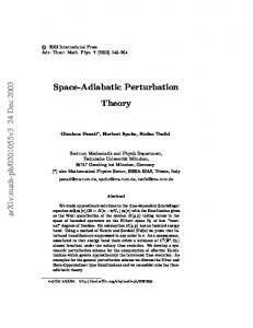
On the second line we noticed that the second term vanishes as the summing of sines and cosines over j, fortunately, gives zero. Let us now concentrate a little on the sign of the hopping probability t. From Eq. (5.14) we see that the eigenenergy corresponding to the diagonal Hamiltonian is ! πk �k = 2t cos . N+1
(5.15)
In Fig. 5.2 we have a plot of the energy �k against k with the hopping probability t being negative. We see that by taking t < 0 the lowest energy is obtained with k = 1. We may then see how the ground-state wavefunction looks like, by substituting k = 1 into Eq. (5.7) r ϕ1 ( j) =
! πj 2 sin , N+1 N+1
(5.16)
which has no nodes and is spread along the whole N-site chain. This kind of smooth behaviour for the ground-state wavefunction is naturally desired, and it would be a good choice to take t < 0 to attain this particular behaviour. The choice for the sign of the hopping probability t therefore arises from the choice of orbitals with respect to we are expanding our Hamiltonian. If, however, we chose t > 0 then the cosine curve in Fig. 5.2 would be the other way around, and
Chapter 5. Model system: molecule and chain
εk
62
k=1
k=N
k
Figure 5.2: Energy eigenvalue �k for the diagonal Hamiltonian with respect to k with the hopping probability t being negative. then the lowest-energy state is obtained when k = N. With k = N the ground-state wavefunction would, in contrast, have N nodes between the first and the last site of the chain. All in all, we have obtained a Hamiltonian for the TB chain that is diagonal, and that the operator dˆ† is a “ladder” operator that maps an eigenstate of Hˆ ch with energy E onto another eigenstate k,σ
with energy E + �k . This statement is easily verified: If Hˆ ch |Ei = E|Ei, then =0
z }| {� � † † † † Hˆ ch dˆk,σ |Ei = Hˆ ch dˆk,σ −dˆk,σ Hˆ ch + dˆk,σ Hˆ ch |Ei �h i � = Hˆ ch , dˆ†k,σ + dˆ†k,σ Hˆ ch |Ei � � = �k dˆ†k,σ + Edˆ†k,σ |Ei
= (E + �k ) dˆ†k,σ |Ei ⇒
dˆ†k,σ |Ei = |E + �k i .
(5.17)
For the vacuum state |0i we have dˆk,σ |0i = 0, ∀k, σ. The general form of the eigenstate of Hˆ ch therefore reads XX� �nk � �nk |Ei = N dˆ†k1 ,σ 1 dˆ†k2 ,σ 2 . . . |0i , (5.18) n o σ n ,... k1
where N is a normalization factor, and the energy of this state is E = (since we are studying fermions).
P
k nk �k
with nk = {0, 1}
So far, we have considered the case with N-site chain, and obtained a diagonal Hamiltonian in Eq. (5.14). For small systems this can be solved analytically by pen and paper, and for this purpose we consider a truncated chain with only two sites. Now that N = 2 we have
5.2. Solving the eigenvalue problem �k = 2t cos
�
π 3k
63
� . Then we have for the Hamiltonian
Hˆ ch =
2 XX σ k =1
�k dˆ†k,σ dˆk,σ
� �� � �� � � π ˆ† ˆ 2π ˆ† ˆ † ˆ ˆ d1,+ d1,+ + d1,− d1,− + 2t cos d2,+ d2,+ + dˆ†2,− dˆ2,− = 2t cos 3 3 | {z } | {z } =1/2
=−1/2
= t (nˆ 2,+ + nˆ 2,− − nˆ 1,+ − nˆ 1,− ) .
(5.19)
Then we need to construct all the possible states for two electrons occupying the two sites, i.e., the eigenstates |1i = dˆ†1,+ dˆ†1,− |0i ,
|2i = dˆ†1,+ dˆ†2,− |0i ,
|3i = dˆ†1,− dˆ†2,+ |0i ,
|4i = dˆ†2,+ dˆ†2,− |0i .
(5.20)
Because the Hamiltonian is diagonal, we get the corresponding eigenenergies simply as hi|Hˆ ch |ii with i ∈ [1, 4]: h1|Hˆ ch |1i = 2t ,
5.2.2
h2|Hˆ ch |2i = 0 ,
h3|Hˆ ch |3i = 0 ,
h4|Hˆ ch |4i = −2t .
(5.21)
Two-site molecule
For the molecule we have the (diagonal) Hamiltonian in Eq. (5.3). The creation and annihilation ˆ respectively. The number operators for the electrons on the molecular orbitals are bˆ † and b, of electrons on the LUMO and HOMO levels is essential. Because there is two states for the electrons to be located, the number of interacting electrons can be from one to four. These four cases need to be considered separately. For the one-electron case there is only two different configurations: |1i = bˆ †H,+ |0i ,
|2i = bˆ †L,+ |0i .
(5.22)
The other possibilities with “spin down” electrons are essentially the same because the physical properties of the system do not change by choosing the direction of the spin. This is of course different when there is more than one electron to be considered. When operating with Hˆ mol to the states in Eq. (5.22) we get the eigenenergies h1|Hˆ mol |1i = ξH ,
h2|Hˆ mol |2i = ξH + ∆0 .
(5.23)
For the two-electron case there is four different configurations: |1i = bˆ †H,+ bˆ †H,− |0i ,
|2i = bˆ †H,+ bˆ †L,− |0i ,
|3i = bˆ †H,− bˆ †L,+ |0i ,
|4i = bˆ †L,+ bˆ †L,− |0i .
(5.24)
Now the physical situation between the second and the third ket would change when interchanging the spin labels. This is due to the fact that the direction for the spin needs to be fixed (although it can be chosen arbitrarily) whereas in the one-electron case the spins were pointing only in one direction. The corresponding eigenenergies are readily calculated (note, however, that the energies of the second and the third state are the same) h1|Hˆ mol |1i = 2ξH + U0 , h2|Hˆ mol |2i = 2ξH + ∆0 + UHL , h3|Hˆ mol |3i = 2ξH + ∆0 + UHL , h4|Hˆ mol |4i = 2ξH + 2∆0 + U0 .
(5.25)
Chapter 5. Model system: molecule and chain
64
The calculation for the three-electron case goes identically as above but now we have only two different states: |1i = bˆ † bˆ † bˆ † |0i , |2i = bˆ † bˆ † bˆ † |0i . (5.26) H,+ H,− L,+
H,+ L,+ L,−
The molecular orbital with only one electron could also have the same electron but with the opposite spin. These two extra configurations would not add anything new to the system because the other molecular orbital has already two electrons with opposite spins, i.e., interchanging the directions of the spins gives the same state. The eigenenergies corresponding to the eigenstates in Eq. (5.26) are h1|Hˆ mol |1i = 3ξH + ∆0 + U0 + 2UHL ,
h2|Hˆ mol |2i = 3ξH + 2∆0 + U0 + 2UHL .
(5.27)
The molecule can also have four electrons but in this case it is fully occupied, and therefore only one electron configuration is possible: |1i = bˆ †H,+ bˆ †H,− bˆ †L,+ bˆ †L,− |0i .
(5.28)
h1|Hˆ mol |1i = 4ξH + 2∆0 + 2U0 + 4UHL .
(5.29)
The energy of this state is
We may now pay a little more attention to the parameters introduced in the molecular energy spectrum. We consider ξH to be the lowest energy level and therefore use ∆0 > 0. Also the parameters for the Coulomb repulsion (U0 and UHL ) are taken positive. Then choose the two-particle state |1i in Eq. (5.24) to be the ground state. The ground-state energy is to be the smallest, hence, comparing the ground state to the one-particle state |1i in Eq. (5.22) gives 2ξH + U0 < ξH
ξH < −U0 .
⇒
(5.30)
We can also deduce that two particles in the HOMO level must be lower in energy than one particle in the HOMO level and one particle in the LUMO level [|2i and |3i in Eq. (5.24)], i.e., 2ξH + U0 < 2ξH + ∆0 + UHL
⇒
∆0 + UHL > U0 .
(5.31)
Clearly, the ground state must also be lower in energy than a three-particle state |1i in Eq. (5.26), i.e., 2ξH + U0 < 3ξH + ∆0 + U0 + 2UHL
⇒
ξH > −∆0 − 2UHL .
(5.32)
We have now got [from Eqs. (5.30) and (5.32)] a range of values for the energy in HOMO level − ∆0 − 2UHL < ξH < −U0 ,
(5.33)
where also the condition from Eq. (5.31) is fulfilled since −∆0 − 2UHL = −(∆0 + UHL ) − UHL < −U0 − UHL < −U0 . A convenient choice for the Eq. (5.32) to be satisfied is when we have ξH = −
∆0 U0 − − UHL . 2 2
(5.34)
5.2. Solving the eigenvalue problem
5.2.3
65
Interaction between the molecule and the chain
The interaction term of the total Hamiltonian is in Eq. (5.4). We consider first the case with thyb = 0, i.e., the molecule and the chain interact only via the term Uext . This approximation can be solved analytically. The number operator in the terminal site of the chain nˆ ch needs to be converted to the basis we defined in Eqs. (5.5) and (5.6). We have then X nˆ ch = cˆ†1,σ cˆ1,σ σ
=
! ! πj 2 XX πk sin sin dˆ† dˆj,σ . N+1 σ N+1 N + 1 k,σ
(5.35)
j,k
We then get back to our truncated-chain example, and take two energy levels (j, k = 1, 2) and two sites (N = 2). Then we have for the number operator in the terminal site of the chain √ = 3/2
nˆ ch =
√ = 3/2
√ = 3/2
z }| { z }| { z }| { z }| { � � � � � � � � 2 Xh π π ˆ† ˆ π 2π ˆ† ˆ sin sin d1,σ d1,σ + sin d d2,σ sin 3 σ 3 3 3 3 1,σ � � � � � � � � 2π π ˆ† ˆ 2π 2π ˆ† ˆ i d2,σ d1,σ + sin d d2,σ + sin sin sin 3 3 3 3 2,σ | {z } | {z } | {z } | {z } √ = 3/2
=
√ 3/2
√ = 3/2
√ = 3/2
√ = 3/2
� 1� nˆ 1 + nˆ 2 + dˆ†1,+ dˆ2,+ + dˆ†2,+ dˆ1,+ + dˆ†1,− dˆ2,− + dˆ†2,− dˆ1,− . 2
(5.36)
With Eq. (5.36) we can rewrite Eq. (5.4) (when thyb = 0) as � � � � 1 Vˆ = Uext (nˆ mol − 2) nˆ 1 + nˆ 2 + dˆ†1,+ dˆ2,+ + dˆ†2,+ dˆ1,+ + dˆ†1,− dˆ2,− + dˆ†2,− dˆ1,− − 1 . 2
(5.37)
The operator nˆ mol in Eq. (5.37) is already in correct basis, i.e, it gives only the number of electrons on the molecule. From this we can deduce that when there is two electrons on the molecule, the interaction vanishes. We can now study different systems with our two-site molecule and two-site chain. The simplest case is to put one electron to the molecule and one electron to the chain. For this set-up we can distinguish four different electron configurations |1i = bˆ †H,+ dˆ†1,+ |0i ,
|2i = bˆ †H,+ dˆ†2,+ |0i ,
|3i = bˆ †L,+ dˆ†1,+ |0i ,
|4i = bˆ †L,+ dˆ†2,+ |0i .
(5.38)
The different combinations for the spin index do not give any extra information about the system, because the electron on the molecule cannot depend on the spin of the electron on the chain, and vice versa. Operating to the eigenkets in Eq. (5.38) with the total Hamiltonian operator [in Eq. (5.1)] we get the Hamiltonian matrix whose eigenvalues are the eigenenergies of the system. Because the Hˆ ch and Hˆ mol parts of the Hamiltonian are diagonal, the contribution from these is readily calculated [in fact, for the molecule we already calculated the eigenenergies in Eq. (5.23)] Hˆ ch |1i = t|1i ,
Hˆ ch |2i = −t|2i ,
Hˆ ch |3i = t|3i ,
Hˆ ch |4i = −t|4i ,
(5.39)
Hˆ mol |1i = ξH |1i , Hˆ mol |2i = ξH |2i , Hˆ mol |3i = (ξH + ∆0 ) |3i , Hˆ mol |4i = (ξH + ∆0 ) |4i . (5.40)
Chapter 5. Model system: molecule and chain
66
For the interaction part, we have to operate with Eq. (5.37) to the states in Eq. (5.38). From this calculation we get (note that hnˆ mol i = 1) ˆ V|1i = ˆ V|2i = ˆ V|3i = ˆ V|4i =
1 Uext |1i + 2 1 Uext |2i + 2 1 Uext |3i + 2 1 Uext |4i + 2
1 Uext |2i 2 1 Uext |1i 2 1 Uext |4i 2 1 Uext |3i . 2
We are now ready to write down the total Hamiltonian matrix h1|Hˆ tot |1i ˆ � � h2|Htot |1i ˆ Htot = ij h3|Hˆ |1i tot ˆ h4|Htot |1i
h1|Hˆ tot |2i h1|Hˆ tot |3i h1|Hˆ tot |4i h2|Hˆ tot |2i h2|Hˆ tot |3i h2|Hˆ tot |4i h3|Hˆ tot |2i h3|Hˆ tot |3i h3|Hˆ tot |4i h4|Hˆ tot |2i h4|Hˆ tot |3i h4|Hˆ tot |4i
1 t + ξH + 1 Uext U 0 0 2 2 ext 1 1 U −t + ξ + U 0 0 H 2 ext 2 ext . (5.41) = 1 1 0 0 t + ξ + ∆ + U U H 0 ext ext 2 2 1 1 0 0 −t + ξH + ∆0 + 2 Uext 2 Uext The matrix in Eq. (5.41) is block diagonal, and the diagonalization of the matrix can be done separately for the two-by-two parts. The eigenenergies are E1,2 = E3,4
1 2ξH + Uext ± 2
!
q 4t2
2
+ Uext ! q 1 2 2 = 2ξH + ∆0 + Uext ± 4t + Uext . 2
(5.42) (5.43)
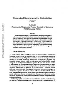
By this manner, we can construct the Hamiltonian matrices for all systems we want to study. Finding the eigenenergies of the studied system is then a matter of diagonalizing the Hamiltonian matrix. As an example, we calculate the lowest energies (ground-state energies) for a system of two electrons on the chain with varying number of electrons on the molecule. We use parameter values U0 = UHL = ∆0 = −t = 1 with ξH = −2 and plot the ground-state energies versus the number of electrons on the molecule Nmol with different values of Uext in Fig. 5.3a. We also calculate the electron densities in the terminal site of the chain from the corresponding electron wave function in Fig. 5.3b.2 Let us then look at an application of the studied model. Consider the system of two-site molecule and two-site chain to be two electrons on the molecule and two electrons on the chain. The ground state of this system is, naturally, the electrons occupying the states that are the lowest in energy: 2 This
calculation is explained more in detail in Sec. 5.5 on page 86.
5.2. Solving the eigenvalue problem
67
-2 Uext = 0.0 Uext = 0.5 Uext = 1.0 Uext = 1.5 Uext = 2.0
-2.5
EGS
-3 -3.5 -4 -4.5 -5 0
1
2 nmol
3
4
(a) Ground-state energies versus the number of electrons in the molecule.
2
Uext = 0.0 Uext = 0.5 Uext = 1.0 Uext = 1.5 Uext = 2.0
1.8 1.6 1.4
nch
1.2 1 0.8 0.6 0.4 0.2 0 0
1
2 nmol
3
4
(b) Electron densities in the terminal site of the chain versus the number of electrons in the molecule.
Figure 5.3: (a) Ground-state energies in a system of two electrons on the chain, (b) electron densities in the terminal site of the chain.
Chapter 5. Model system: molecule and chain
68
|Ψ0 i = bˆ †H,+ bˆ †H,− dˆ†1,+ dˆ†1,− |0i Since we have two electrons on the molecule, the interaction between the molecule and the chain vanishes as nˆ mol − 2 = 0 in Eq. (5.4). We can then simply state that the ground state energy is given by [see Eqs. (5.21) and (5.25)] Hˆ tot |Ψ0 i = E0 |Ψ0 i
with
E0 = 2ξH + U0 + 2t .
(5.44)
Then we add one electron to the molecule which will then occupy the LUMO level as the HOMO level is already fully occupied. We hereby have the molecular state |Ψmol i = bˆ †H,+ bˆ †H,− bˆ †L,+ |0i .
(5.45)
Now hnˆ mol i = 3 and the interaction between the molecule and the chain is not zero anymore. In fact, the interaction becomes repulsive as the molecule becomes negatively charged, and therefore the electrons on the terminal site of the chain are being pushed away from the molecule. The two electrons on the chain can arrange themselves in four different combinations as in Eq. (5.20). To evaluate the energies of the whole system, we need to add the contribution from the interaction, as we did when we calculated the eigenenergies in Eq. (5.42). We can now similarly construct all the different electron configurations and operate to these states with Hˆ tot in order to obtain the total Hamiltonian matrix. The energies of the system are again found by evaluating the eigenvalues of the Hamiltonian matrix. This is a straightforward calculation and we state here the results for the eigenvalues. As there is four different states that the electrons on the chain can form, we have four eigenvalues, and two of them are the same because kets |2i and |3i in Eq. (5.20) are same in energy. We then have E1 = 3ξH − ∆0 + U0 + 2UHL −
q 4t2 + Uext 2
(5.46)
E2 = 3ξH − ∆0 + U0 + 2UHL
(5.47)
E3
(5.48)
q = 3ξH − ∆0 + U0 + 2UHL + 4t2 + Uext 2 ,
where E1 corresponds to a state with both electrons on the chain being on the lower energy level, E2 to a state with the two electrons on the chain being on different energy levels, and E3 to a state with both electrons on the chain being on the higher energy level. We can now calculate the energy difference between the ground state (two electrons on the molecule and two electrons on the chain) and the added-electron states. These energy differences give us the addition energies of the (hnˆ mol i = 3) -system. Taking parameters −t = ∆0 = U0 = UHL = 1 and ξH = −2 [see Eq. (5.34)] we have from Eqs. (5.44), (5.46), (5.47) and (5.48) ∆1
q = E1 − E0 = 3 − 4 + Uext 2
(5.49)
∆2 = E2 − E0 = 3
(5.50)
∆3
(5.51)
q = E3 − E0 = 3 + 4 + Uext 2 .
We will get back to these results later in Chap. 6 with the corresponding results from the perturbation-theory calculations.
5.3. Solution via perturbative expansion
5.3
69
Solution via perturbative expansion
In Sec. 5.2 we were studying our model exactly with the formalism of second quantization. We can also apply the formalism of many-particle perturbation theory to this particular model. In this manner, we first need to construct the non-interacting Green’s function, G0 , for our system – the molecule and chain. After this, we can compute the self-energy Σ from the Feynman diagrams, and finally apply the Dyson equation to obtain the total Green’s function. Our goal is to evaluate the addition energies of the system as we did in the previous section in Eqs. (5.49), (5.50) and (5.51). Although the perturbation-theoretical approach to this small system is quite an overkill, it is an educational study of the functionality of the perturbation theory. When we treat our N-particle system perturbatively, we get information about the N − 1 and N + 1 particle systems without ever calculating them explicitly.
5.3.1
Non-interacting Green’s function for the molecule
We start with the definition G0(1) (x, z; x0 , z0 ) = ihΨ0 |TC [ψˆ H (x, z)ψˆ †H (x0 , z0 )]|Ψ0 i ,
(5.52)
where TC is the time-ordering operator for which TC [A(z)B(z0 )] = θ(z − z0 )A(z)B(z0 ) − θ(z0 − z)B(z0 )A(z) , with
1 θ(z) = 0
when z ≥ 0 when z < 0
(5.53)
(5.54)
being the Heaviside step function. The subscripts H stand for Heisenberg operators, and the spin index σ is included in the x coordinate by x = (r, σ). As we are dealing only with one-particle Green’s functions here, no mix-ups should occur if we omit the subscript notation in Eq. (5.52) and write simply G0 . We can express the field operators in a the molecular orbital basis by X (∗) (†) ψˆ †H (x, z) = ϕk,σ (r)bˆ k,σ,H (z) , (5.55) k,σ
where the parentheses around † and ∗ mean that we have definitions for both creation and annihilation operators. We also emphasize that these creation and annihilation operators correspond to the molecule as in Hamiltonian (5.3). We can transform from Heisenberg picture into Schrodinger picture by writing the Heisenberg operators as ¨ ˆ ˆ (†) ψˆ H (x, z) = eiH0 z ψˆ (†) (x, z)e−iH0 z ,
(5.56)
where Hˆ 0 is the time-independent Hamiltonian. With Eq. (5.56) we get ˆ ˆ (†) (†) bˆ k,H (z) = eiH0 z bˆ k (z)e−iH0 z .
(5.57)
Now insert these expressions into Eq. (5.52) Xh ˆ ˆ ˆ 0 ˆ 0 G0 (x, z; x0 , z0 ) = i θ(z − z0 )ϕk,σ (r)ϕ∗k0 ,σ0 (r0 )hΨ0 |eiH0 z bˆ k,σ (z)e−iH0 z eiH0 z bˆ †k0 ,σ0 (z0 )e−iH0 z |Ψ0 i k,k0 σ,σ0
i ˆ 0 ˆ 0 ˆ ˆ − θ(z0 − z)ϕ∗k0 ,σ0 (r0 )ϕk,σ (r)hΨ0 |e−iH0 z bˆ †k0 ,σ0 (z0 )eiH0 z e−iH0 z bˆ k,σ (z)eiH0 z |Ψ0 i . (5.58)
Chapter 5. Model system: molecule and chain
70
We may also insert a complete set of N + 1 and N − 1 particle states, in the form of into this expression
P
n |Ψn ihΨn |
= 1,
G0 (x, z; x0 , z0 )
= i
Xh
ˆ ˆ ˆ 0 +1 +1 −iHˆ 0 z0 ˆ † θ(z − z0 )ϕk,σ (r)ϕ∗k0 ,σ0 (r0 )hΨ0 |eiH0 z bˆ k,σ (z)e−iH0 z |ΨN ihΨN bk0 ,σ0 (z0 )e−iH0 z |Ψ0 i |e n n
k,k0 σ,σ0 n,m ˆ 0 ˆ 0 ˆ 0 N−1 −iHˆ 0 z ˆ − θ(z0 − z)ϕ∗k0 ,σ0 (r0 )ϕk,σ (r)hΨ0 |eiH0 z bˆ †k0 ,σ0 (z0 )e−iH0 z |ΨN−1 bk,σ (z)e−iH0 z |Ψ0 i m ihΨm |e X� N +1 0 +1 +1 ˆ † = i θ(z − z0 )ϕk,σ (r)ϕ∗k0 ,σ0 (r0 )ei(E0 −En )(z−z ) hΨ0 |bˆ k,σ (z)|ΨN ihΨN |bk0 ,σ0 (z0 )|Ψ0 i n n
i
k,k0 σ,σ0 n,m
� N−1 0 N−1 ˆ − θ(z0 − z)ϕ∗k0 ,σ0 (r0 )ϕk,σ (r)ei(E0 −Em )(z −z) hΨ0 |bˆ †k0 ,σ0 (z0 )|ΨN−1 ihΨ | b ( z ) |Ψ i . (5.59) 0 k,σ m m We notice how the expression in Eq. (5.59) depends on the relative time coordinate τ B z − z0 . For the ground state Ψ0 we are considering a simple Fermi sphere, i.e., a three-dimensional region in momentum space with N particles inside, all having their momentum less than the value corresponding to the surface of the sphere. Then we deal with the matrix elements inside the sum in Eq. (5.59). The states with N + 1 and N − 1 particles are operated with the annihilation and creation operators bˆ k,σ and bˆ †k0 ,σ0 , respectively. These operations give a non-zero contribution only if we have n = k, k0 and m = k, k0 , and this observation kills the summations over n and m. The contribution from these operations may, or may not, overlap with the ground state Ψ0 , and for this purpose we introduce step functions inside the Fermi sphere. For the N + 1 and N − 1 particle energies we have EN±1 = E0 ± �k . We can then simplify the expression k in Eq. (5.59), with the ideas presented above, as G0 (x, x0 ; τ) = i
X�
E0 −E0 −�k )τ θ(τ)ϕk,σ (r)ϕ∗k0 ,σ0 (r0 )ei(� θ
� �
�
k,k0 σ,σ0
= i
− X
� N − k δk,k0 δσ,σ0 2
�0 +�k )(−τ) � E0 −E θ θ(−τ)ϕ∗k0 ,σ0 (r0 )ϕk,σ (r)ei(�
θ(τ)ϕk,σ (r)ϕ∗k,σ (r0 )e−i�k τ − i
k≤N/2 σ
X
� � � N 0 k − δk,k0 δσ,σ0 2
θ(−τ)ϕ∗k,σ (r0 )ϕk,σ (r)e−i�k τ . (5.60)
k>N/2 σ
Then we insert a useful form of the step function −1 θ(x) = lim + η→0 2πi
Z
∞
−∞
eiλx dλ λ + iη
(5.61)
into Eq. (5.60) to obtain G (x, x ; τ) = i 0
0
X
ϕk,σ (r)ϕ∗k,σ (r0 )
� �Z ∞ 1 eiλτ −i�k τ − dλ e 2πi −∞ λ + iη
ϕ∗k,σ (r0 )ϕk,σ (r)
� �Z ∞ 1 e−iλτ −i�k τ e , − dλ 2πi −∞ λ + iη
k≤N/2 σ
− i
X k>N/2 σ
� � η → 0+ .
(5.62)
5.3. Solution via perturbative expansion
71
Then we take Fourier transforms with respect to the relative time coordinate τ, and evaluate the integrals Z ∞ Z ∞ dλ 1 X ϕk,σ (r)ϕ∗k,σ (r0 ) dτeiωτ eiλτ e−i�k τ G0 (x, x0 ; ω) = − 2π λ + iη −∞ −∞ k≤N/2 σ
+
Z ∞ Z ∞ 1 X ∗ 0 dλ ϕk,σ (r )ϕk,σ (r) dτeiωτ e−iλτ e−i�k τ , 2π −∞ λ + iη −∞
� � η → 0+
k>N/2 σ
=2πδ(ω+λ−�k )
= −
+
1 2π
X
Z ϕk,σ (r)ϕ∗k,σ (r0 )
∞
−∞
k≤N/2 σ
dλ λ + iη
z Z
}|
∞
{
dτei(ω+λ−�k )τ
−∞
Z ∞ Z ∞ 1 X ∗ 0 dλ ϕk,σ (r )ϕk,σ (r) dτei(ω−λ−�k )τ , 2π λ + iη −∞ −∞ k>N/2 | {z } σ
� � η → 0+
=2πδ(ω−λ−�k )
X
= −
Z ϕk,σ (r)ϕ∗k,σ (r0 )
dλ −∞
k≤N/2 σ
+
X
Z ϕ∗k,σ (r0 )ϕk,σ (r)
k>N/2 σ
=
X
ϕk,σ (r)ϕ∗k,σ (r0 )
k≤N/2 σ
=
X
∞
∞
dλ −∞
δ(ω + λ − �k ) λ + iη
δ(ω − λ − �k ) , λ + iη
� � η → 0+
X 1 1 + ϕ∗k,σ (r0 )ϕk,σ (r) , ω − �k − iη ω − �k + iη
� � η → 0+
k>N/2 σ
ϕk,σ (r)ϕ∗k,σ (r0 )
k,σ
1 , ω − �k + iη sgn(�k )
� � η → 0+ .
On the last line we defined +1 when k > N/2 i.e. outside the Fermi sphere, unoccupied sgn(�k ) = −1 when k ≤ N/2 i.e. inside the Fermi sphere, occupied.
(5.63)
(5.64)
We can finally sum over the molecular orbitals to obtain the non-interacting Green’s function for the molecule in frequency space G0k,k0 (ω) = σ,σ0
δk,k0 δσ,σ0 , ω − �k + iη sgn(�k )
� � η → 0+ .
(5.65)
We keep the term η still inside the expression for the non-interacting Green’s function because we eventually want to do Feynman-diagram calculations with the non-interacting Green’s function, and we take the limit η → 0+ after these calculations.
5.3.2
Non-interacting Green’s function for the TB chain
For the TB chain, the derivation of non-interacting Green’s function is slightly different than for the molecule. This is due to the fact that, as in Hamiltonian (5.2), we have the creation
Chapter 5. Model system: molecule and chain
72
and annihilation operators for the chain in site basis and we must transform into energy eigenbasis as done in Sec. 5.2. In the exact calculation we used a linear transformation of the form (5.5), but now we will only refer to a unitary transformation that diagonalizes the tight-binding Hamiltonian. We will find the form of this transformation after we have derived the non-interacting Green’s function. We hereby have X (†) (†) (†) dˆk,σ = U k,l cˆl,σ0 , (5.66) l,σ0
σ,σ0
where U†k,l = U∗l,k is the usual hermitean conjugate of a matrix. Also in this basis, the ground σ,σ0
σ0 ,σ
state is simply a Fermi sphere and we can do the derivation identical to the case of molecule as far as Eq. (5.59), but we must keep the unitary matrices connected to the creation and annihilation operators. We, thus, expand the field operators in Eq. (5.52) within a basis of functions ϕk,σ (r) and expand the creation and annihilation operators again as in Eq. (5.66). This procedure involves a little more book keeping with the summing indices, and this way we get G0 (x, z; x0 , z0 )
= i
X X�
N +1 0 θ(z − z0 )ϕk,σ (r)ϕ∗k0 ,σ0 (r0 )ei(E0 −En )(z−z ) ×
k,k0 l,l0 σ1 ,σ01 σ2 ,σ02 m n N +1 +1 ∗ ihΨN |U l0 ,k0 cˆ†l0 ,σ0 (z0 )|Ψ0 i k,l cˆl,σ2 (z)|Ψn n 2 σ1 ,σ2 σ0 ,σ0
× hΨ0 |U
2
− θ(z
0
N−1 0 − z)ϕ∗k0 ,σ0 (r0 )ϕk,σ (r)ei(E0 −Em )(z −z)
×
N−1 × hΨ0 |U∗l0 ,k0 cˆ†l0 ,σ0 (z0 )|ΨN−1 m ihΨm |U σ02 ,σ01
1
k,l σ1 ,σ2
2
� cˆl,σ2 (z)|Ψ0 i .
(5.67)
Also in this case, we write the step functions by using Eq. (5.61) and Fourier transform with respect to the relative time coordinate τ B z − z0 . We also notice that the sums over n and m are done away with the fact that n = l, l0 and m = l, l0 . First we get X X G0 (x, z; x0 , z0 ) = i θ(τ)ϕk,σ (r)ϕ∗k0 ,σ0 (r0 )e−i�l τ U k,l U∗l0 ,k0 δl,l0 δσ2 ,σ02 σ1 ,σ2
k,k0 l,l0 ≤N/2 σ1 ,σ01 σ2 ,σ02 m n
− i
X X k,k0 l,l0 >N/2 σ1 ,σ01 σ2 ,σ02 m n
σ02 ,σ01
θ(−τ)ϕk,σ (r)ϕ∗k0 ,σ0 (r0 )e−i�l τ U∗l0 ,k0 U σ02 ,σ01
k,l δl,l0 δσ2 ,σ02 σ1 ,σ2
,
(5.68)
and then we Fourier transform and insert the definition for the step function to obtain [the evaluation of the integrals goes exactly the same way as in Eq. (5.63)] X � � 1 ϕk,σ1 (r)ϕk0 ,σ01 (r0 )U k,l U∗ l,k0 η → 0+ G0 (x, x0 ; ω) = , σ1 ,σ2 σ ,σ0 ω − �l + iη sgn(�l ) 0 k,k l,σ2
2
∗ k,l U l,k0 σ1 ,σ2 σ2 ,σ01
1
U ⇒
G0k,k0 (ω) = σ1 ,σ01
X l,σ2
ω − �l + iη sgn(�l )
,
� � η → 0+ .
In this case the sign of iη is + for an excited state, and − for the ground state.
(5.69)
5.3. Solution via perturbative expansion
5.3.3
73
Hamiltonian and interactions
As we are dealing with calculations that include expansions of the interaction, we would want to keep the interactions as simple as possible, and include the more complicated terms inside the Hamiltonian. The interaction part of the Hamiltonian in Eq. (5.4), Uext (nˆ ch − 1) (nˆ mol − 2), contains both one-particle and two-particle terms. We would like this term to be in the form of Uext nˆ ch nˆ mol so that we could handle the interactions with j i
" l
k
Vi jkl = Vi j δi,l δ j,k .
(5.70)
Expanding the term in Eq. (5.4) we get
Vˆ = Uext (nˆ ch nˆ mol − 2nˆ ch − nˆ mol + 2) ,
(5.71)
where the number operator on the molecule is nˆ mol = nˆ H + nˆ L . These terms we can adapt to the molecular part of the Hamiltonian, i.e., we get for the Eq. (5.3) Hˆ˜ mol = (ξH − Uext ) nˆ H + (ξH + ∆0 − Uext ) nˆ L + U0 nˆ H,+ nˆ H,− + U0 nˆ L,+ nˆ L,− + UHL nˆ H nˆ L . (5.72) There is also a constant term in Eq. (5.71), 2Uext , which we will neglect as adding a constant to the Hamiltonian does not change its properties. The third term to be considered is −2Uext nˆ ch , which unfortunately cannot be included in the other parts of the Hamiltonian. But, fortunately, we can take this term into account when calculating the self-energy. This idea is seen from the Dyson equation. We define the non-interacting Green’s function G0 through � � i∂t − hˆ (1) G0 (1, 10 ) = δ(1, 10 ) , (5.73) and the full Green’s function G through Z � � 0 0 i∂t − hˆ (1) − δV G(1, 1 ) = δ(1, 1 ) + d2 Σ(1, 2)G(2, 1) ,
(5.74)
ˆ (In our case δV is where δV is a small perturbation that is not included in the Hamiltonian h. the part we could not include in the Hamiltonian, i.e., −2Uext nˆ ch .) We can manipulate Eq. (5.74) by moving the δV term to the other side of the equation. In this way we get Z � � 0 0 ˆ i∂t − h(1) G(1, 1 ) = δ(1, 1 ) + d2 [Σ(1, 2) + δ(1, 2)δV ] G(2, 1) . (5.75) | {z } CΣ0
This trick is completely allowed since the solution of the Dyson equation remains as G = G0 + G0 Σ0 G , (5.76) � � as can be checked by operating from left with i∂t − hˆ (1) . The term to be added to the self-energy is then simply a constant −2Uext regarding the first site of the chain, i.e., 0 0 0 0 0 0 0 0 . (5.77) δVi j = 0 0 −2U ext 0 0 0 0 0
Chapter 5. Model system: molecule and chain
74
5.3.4
Two-site molecule and two-site TB chain
For this particular system of a two-site molecule next to a two-site TB chain we can determine the non-interacting Green’s function G0 by means of Eqs. (5.65) and (5.69). We take the indices for the G0 matrix to be as i, j ∈ {H, L, 1, 2}, where H and L refer to the HOMO and LUMO levels of the molecule, respectively, and 1 and 2 refer to the first and second site of the chain. For the molecule part, the matrix is diagonal as Eq. (5.65) indicates, and we only need to insert proper energies in �k . For the two-site chain, the Hamiltonian matrix is 0 −t � � , Hˆ ch = ij −t 0
(5.78)
where t is the hopping probability. A unitary matrix that diagonalizes this matrix is given by 1 1 1 . Ui j = √ 2 1 −1
(5.79)
Hence, we have from Eq. (5.69) for the chain part 1 1 1 1 ω−�1 −iη G0i j (ω) = √ 2 1 −1 0
0 1 1 1 , √ 2 1 1 −1 ω−�2 +iη
(5.80)
where �1 = t and �2 = −t (as we are using t < 0, see Fig. 5.2). The product of matrices yields � � 1 1 1 + 2 ω−t−iη ω + t + iη G0i j (ω) = � � 1 1 1 − 2 ω−t−iη ω+t+iη
1 2
�
1 ω−t−iη
−
1 ω+t+iη
1 2
�
1 ω−t−iη
+
1 ω+t+iη
� � .
(5.81)
We can then finally conclude that the non-interacting Green’s function for our (2 + 2)-site system is 1 0 0 0 ω−ξH +Uext −iη 1 0 0 0 ω−ξH −∆0 +Uext +iη 0 Gi j (ω) = � � � � . (5.82) 1 1 1 1 1 1 0 0 2 ω−t−iη + ω+t+iη 2 ω−t−iη − ω+t+iη � � � � 1 1 1 1 1 1 0 0 2 ω−t−iη − ω+t+iη 2 ω−t−iη + ω+t+iη It is now worth mentioning how the extra Uext terms appear in the energies of the molecule as explained earlier in Eq. (5.72). For the interaction matrix we have U0 UHL Uext UHL U0 Uext Vi j = U 0 ext Uext 0 0 0
0 0 . 0 0
(5.83)
5.3. Solution via perturbative expansion
5.3.5
75
Self-energy calculations
Now we are ready to do an actual Feynman-diagram calculation. We first consider the Hartree– Fock approximation for the self-energy, i.e., we calculate only the tadpole and exchange diagrams in first order. In the following we have a non-interacting Green’s function G0 (ω) joining the diagram at point j and leaving at point i. In every vertex, the frequency must be conserved, and every internal index must be summed over as well as every internal frequency must be integrated over. ω−ν 1 0 ω l k ν HF −2Uext j + + i Σi j (ω) = k l 0 ω ij ij
#$ %
=Vil δi,k δl,j δσi ,σk δσl ,σ j
=Vik δi,j δk,l δσi ,σ j δσk ,σl
= −i
XZ k,l σk ,σl
∞
∞
dω0 2π
z}|{ XZ iω0 η 0 0 e Gkl (ω ) Vikl j +i σi σk σl σ j
k,l σk ,σl
∞
−∞
z}|{ dν iνη 0 e Glk (ν) Vil jk −2Uext δi,1 δ j,1 2π σi σl σ j σk
Z XZ dω0 0 dν iνη 0 iω η 0 0 = −i e Gkk (ω )Vik δi,j δσi ,σ j + i e G ji (ν)Vi j − 2Uext δi,1 δ j,1 . (5.84) 2π 2π k,σk
From the expression in Eq. (5.84) we can calculate all the different components of the self-energy. All in all, we end up having to calculate 16 different elements, but fortunately, most of them are zero and that can be seen easily. It is also worthwile to notice that we now include the term discussed in Eq. (5.74) to the self-energy. In the first approximation only ΣHH and ΣLL are non-zero. Let us calculate the ‘HH’ component as an example. By inserting i, j = H into expression in Eq. (5.84) and using Eqs. (5.82) and (5.83) we get Z i dω0 iω0 η h 0 HF ΣHH (ω) = −2i e GHH (ω0 )VHH + G0LL (ω0 )VHL + G011 (ω0 )VH1 + G022 (ω0 )VH2 2π Z dν iνη 0 +i e GHH VHH 2π " Z UHL U0 dω0 iω0 η e + 0 = −2i 0 2π ω − ξH + Uext − iη ω − ξH − ∆0 + Uext + iη � �# 1 Uext 1 + + 2 ω0 − t − iη ω0 + t + iη Z dν iνη U0 +i e . (5.85) 2π ν − ξH + Uext − iη Now we use Cauchy’s integral formula (see Sec. 4.1) to calculate these integrals. We need the formula derived in Eq. (4.17) and also the idea from Eq. (4.22). We see that the terms with iη positive vanish, as these correspond to poles in the LHP, and the exponential convergence factor forces the integration via the UHP. Hence, we obtain � � 1 Uext 1 ΣHF 2πi U + + i 2πiU0 ( ω ) = −2i 0 HH 2π 2 2π = U0 + Uext . (5.86)
Chapter 5. Model system: molecule and chain
76
Similarly, we can calculate the ‘LL’ component. All the other components give zero contribution, but it is essential to notice, that the tadpole diagram gives contribution 2Uext to the ‘11’ component, which is then exactly cancelled by the added extra term in Eq. (5.77). This gives us the self-energy matrix for the first step of the calculation U0 + Uext 0 0 2UHL + Uext HF(1) Σi j (ω) = 0 0 0 0
0 0 0 0 . 0 0 0 0
(5.87)
We can then insert the self-energy into Dyson equation to obtain the total Green’s function for the first step HF(1) Gi j (ω)
�� �−1 �−1 HF(1) 0 = Gi j (ω) − Σi j (ω) 1 0 0 ω−ξH −U0 1 0 0 ω−ξH −∆0 −2UHL = � � 1 1 0 0 + ω+1t+iη 2 ω−t−iη � � 1 1 1 0 0 2 ω−t−iη − ω+t+iη
0 � � . 1 1 1 2 ω−t−iη − ω+t+iη � � 1 1 1 + 0
2
ω−t−iη
(5.88)
ω+t+iη
The next step of the calculation is to take the derived Green’s function GHF(1) and to calculate the first order diagrams again, but this time with the new Green’s function as a propagator. As an example, we calculate here the ‘LL’ component of the second step: " Z U0 dω0 iω0 η UHL HF(2) ΣLL (ω) = −2i e + 0 0 2π ω − ξH − U0 − iη ω − ξH − ∆0 − 2UHL + iη �# � 1 Uext 1 + + 2 ω0 − t − iη ω0 + t + iη Z dν iνη U0 +i e . (5.89) 2π ν − ξH − ∆0 − 2UHL + iη Again we use Cauchy’s integral formula, and see that the terms with iη positive vanish due to the orientation of the integration path. Simplifying the terms we obtain HF(2)
ΣLL
(ω) = 2UHL + Uext ,
(5.90)
which is exactly the same result we got in the first step of the calculation. The same thing happens with all the other components as well. This implies that the perturbation sum converged after the first step of the calculation, and the Green’s function we got in Eq. (5.88) is the full HF Green’s function. From the poles of the GHH (ω) and GLL (ω) components in Eq. (5.88) we find the removal and additional spectrum in the HOMO and LUMO levels, respectively. In Hartree–Fock approximation the LUMO spectral peaks then occur at ω = ξH + ∆0 + 2UHL ,
(5.91)
5.3. Solution via perturbative expansion
77
which gives ω = 1 when we take −t = ∆0 = U0 = UHL = 1 and ξH = −2 [see Eq. (5.34)]. We notice that HF approximation does not see the interaction between the molecule and the chain as there is no dependency on the interaction strength Uext in the addition energies. We also notice that when we compare this addition energy to the ones in Eqs. (5.49), (5.49) and (5.49), that HF approximation gives only one peak, whereas the exact result gives three peaks. Next we would like to make our approximation better by calculating more terms in the perturbation series. After the HF calculations we can insert the obtained HF Green’s function into second order diagrams. First, we introduce a second order diagram called the bubble diagram (here also a non-interacting Green’s function G0 (ω) joins the diagram at j and leaves the diagram at i)
ΣHFB i j (ω)
=
ω0 i
ω0 + ν
& q
p
ν
s
r
ω − ω0
l
k
ω0 j
=Vip δi,l δp,q δσ ,σ δσp ,σq
i l X Z dω0 Z dν z}|{ Vipql = −1 · i2 2π 2π σi σp σq σl
k,l,p q,r,s σk ,σl ,σp σq ,σr ,σs
0 HF HF 0 Vksr j GHF kl (ω − ω )Gqs (ν)Grp (ω σk σs σr σ j
+ ν)
|{z}
=Vks δk, j δs,r δσk ,σ j δσs ,σr
X Z dω0 Z dν 0 HF HF 0 = Vip V js GHF i j (ω − ω )Gps (ν)Gsp (ω + ν) . 2π 2π p,s
(5.92)
σp
From this expression we can again calculate all the different elements of the self-energy matrix. The calculations are straightforward although a bit tedious. Let us consider the ‘HH’ component here. We insert i, j = H, GHF from Eq. (5.88), and Vi j from Eq. (5.83) into Eq. (5.92), and this gives Z Z � dω0 dν U0 2 1 1 HFB ΣHH (ω) = 2 0 0 2π 2π ω − ω − ξH − U0 − iη ν − ξH − U0 − iη ω + ν − ξH − U0 − iη
+ +
1 UHL 2 1 0 0 ω − ω − ξH − U0 − iη ν − ξH − ∆0 − 2UHL − iη ω + ν − ξH − ∆0 − 2UHL − iη � � � �� 1 1 1 1 1 1 Uext 2 + + . ω − ω0 − ξH − U0 − iη 2 ν − t − iη ν + t + iη 2 ω0 − t − iη ω0 + ν + t + iη (5.93)
From the expression in Eq. (5.93) we notice that in first two terms inside the square brackets, the integration over ν vanishes as the poles are both in the same side of the complex plane. The only contribution comes from the term with Uext . When we expand the expression inside the parentheses, we again get terms that vanish due to the position of the poles. The only terms that do not vanish are the cross terms, but also the other one from these vanish when we continue to
Chapter 5. Model system: molecule and chain
78
the integration over ω0 . Therefore it is essential to do the calculations very carefully. Note that now we do not have the exponential convergence factor inside the integrals, as we did in the HF calculation. The integrals can therefore be done either in the UHP or in the LHP, and extra attention must be paid in order to get the overall sign correct. Proceeding with the calculation, we have Z Z dω0 dν 1 1 1 Uext 2 HFB ΣHH (ω) = 0 0 2 2π 2π ω − ω − ξH − U0 − iη ν + t + iη ω + ν − t − iη Z 2 0 Uext dω 1 1 = (−i) 0 0 2 2π ω − ω − ξH − U0 − iη ω − 2t − 2iη
= =
i Uext 2 (−i) 2 ω − ξH − U0 − 2t − iη 2 1 2 Uext
(5.94)
.
ω − ξH − U0 − 2t
Similarly we can evaluate the ‘LL’ component, and all in all we have 1U 2 2 ext 0 0 ω−ξH −U0 −2t 2 1 2 Uext 0 HFB(1) ω−ξH −∆0 −2UHL +2t 0 Σi j (ω) = 0 0 0 0 0 0
0 0 . 0 0
(5.95)
Then we insert the evaluated self-energy into Dyson equation to obtain the total Green’s function for the first step in the bubble-diagram calculation. By doing this we get HFB(1) Gi j (ω)
�−1 �� �−1 HFB(1) 0 (ω) = = Gi j (ω) − Σi j
1 1 2 ext ω−ξH −U0 + ω−ξ2 U−U 0 −2t H 0 0 0
0 1
0 0
1U 2 2 ext H −∆0 −2UHL +2t
ω−ξH −∆0 −2UHL − ω−ξ
0 . � � 1 1 1 2 ω−t−iη − ω+t+iη � � 1 1 1 + 0
0
1 2
�
1 ω−t−iη
+
1 ω+t+iη
�
0
1 2
�
1 ω−t−iη
−
1 ω+t+iη
�
2
ω−t−iη
ω+t+iη
(5.96) This is now one step beyond Hartree–Fock approximation; we calculated a second order diagram by using the HF Green’s function. The LUMO spectral peaks again occur at the poles of the HFB(1) GLL (ω). Evaluating the quadratic equation we get two peaks at r
1 1 + Uext 2 2
(5.97)
1 1 + Uext 2 . 2
(5.98)
ω1 = 2 + r ω2 = 2 −
From these we see that by including the bubble diagram in our calculation we now get a clear dependence on the interaction strength Uext . But still, when we compare these addition energies to the ones calculated exactly in Eqs. (5.49), (5.49) and (5.49), we see that one peak is missing.
5.3. Solution via perturbative expansion
79
Usually there is more second order diagrams to be considered. However, in the following we will show that the second order exchange diagram vanishes for the studied system. The exchange diagram in second order is of the form (G0 (ω) joins at j and leaves at i)
' ω2
ΣHFE i j (ω) =
i
ω − ω1 − ω2
ω − ω2
q
p
n
ω − ω1
m
l
j
k
ω1
=Vil δi,q δl,m δσ ,σq δσ ,σm
i l X Z dω Z dω z}|{ 2 1 HF Vilnq Vkpn j GHF (ω − ω1 )GHF = i2 mn (ω − ω1 − ω2 )Gpq (ω − ω2 ) 2π 2π σi σl σn σq σk σp σn σ j kl k,l,m |{z} n,p,q
σk ,σl ,σm σn ,σp ,σq
= −
XZ m,n
=Vkp δk, j δp,n δσk ,σ j δσp ,σn
dω1 2π
Z
dω2 HF HF Vim V jn GHF m j (ω − ω1 )Gnm (ω − ω1 − ω2 )Gin (ω − ω2 ) . (5.99) 2π
If we then try to compute different components of the self-energy, we find that each one of them vanishes. When we integrate over the internal frequency ω2 , we have the second and the third Green’s function with poles at the same side of the complex plane. This is why the integrals over ω2 always vanish in this particular diagram, even if we used the non-interacting Green’s function G0 instead of the HF Green’s function GHF . We can then continue the calculation with the bubble diagram. Next we insert the obtained HFB(1) Green’s function Gi j back to the expression for the self-energy in Eq. (5.92), but first we HFB(1)
HFB(1)
need to factorize the components GHH (ω) and GLL (ω) so that we only get simple poles to be considered in the integration. Since we have two roots ω1 and ω2 for the denominators of the ‘HH’ and ‘LL’ components, we can modify the whole components in the following form HFB(1)
GHH,LL (ω) =
a1 a2 + , ω − ω1 ω − ω2
(5.100)
where a1 and a2 are the factors that we need to find. The procedure itself is a simple algebraic manipulation, and we find the factors for the ‘HH’ component to be a1 =
1 1 − p , 2 4 + 2Uext 2
a2 =
1 1 + p , 2 4 + 2Uext 2
with roots of the denominator as r ω1 = −2 −
1 1 + Uext 2 , 2
(5.101)
r ω2 = −2 +
1 1 + Uext 2 . 2
(5.102)
Similarly for the ‘LL’ component we find the factors to be b1 =
1 1 + p , 2 4 + 2Uext 2
b2 =
1 1 − p , 2 4 + 2Uext 2
(5.103)
Chapter 5. Model system: molecule and chain
80
with roots of the denominator as in Eqs. (5.97) and (5.98) r r 1 1 ω2 = 2 + 1 + Uext 2 . ω1 = 2 − 1 + Uext 2 , 2 2
(5.104)
A noteworthy point for the previous-step calculation is that the intensities of the spectral peaks in Eqs. (5.97) and (5.98) P are given P by the calculated factors in Eq. (5.103). For the factors we then naturally have i ai = 1 = i bi . Now we have, for the next-step calculation, the Green’s function which has simple poles, and we can evaluate the integrals again by using Cauchy’s HFB(2) integral formula. The calculation for the Σi j (ω) is again straightforward but rather long, and we hereby state only the result. All the other components except ‘HH’ and ‘LL’ are again zero, and for the non-zero components we find (with −t = ∆0 = U0 = UHL = 1) 1 1 √ 1 √ 1 + + 2 2 2 2 2 Uext 4+2Uext 4+2Uext HFB(2) + (5.105) ΣHH = q q 2 2 2 1 1 ω + 1 + 2 Uext + 4 ω + 1 + 2 Uext + 4 1 1 1 1 √ √ + + 2 2 Uext 2 4+2Uext 2 4+2Uext 2 HFB(2) . + ΣLL = (5.106) q q 2 2 2 1 1 ω + 1 + 2 Uext + 4 ω + 1 + 2 Uext + 4 We then insert the evaluated self-energy into Dyson equation, and obtain the total Green’s function. There is no point in writing down the obtained Green’s function here, as it is quite a cryptic-looking matrix, but instead we are interested in the physical result for the studied model. We then again calculate the poles of the ‘LL’ component to get the addition energy peaks for the LUMO level. These peaks arise at ω1 = 3 , ω2 = 3 − ω3
(5.107) q
4 + Uext 2 , q = 3 + 4 + Uext 2 .
(5.108) (5.109)
Naturally, the second-step calculation shows also a clear correspondence to the interaction strength Uext . Comparing these addition energies to the exact ones in Eqs. (5.49), (5.49) and (5.49), we see that the difference is already zero, i.e., the perturbation series does not have any more diagrams with these particular initial conditions. This seems more like a coincidence, since when we apply the next step of the calculation we get closer to the so-called GW approximation which takes into account all the bubble diagrams in higher orders also. Now we have three spectral peaks, and we are still able to factorize the components of the obtained Green’s function. This way we can perform yet another step in the calculation, but as we are studying only the bubble diagram, the result found in Eqs. (5.107), (5.108) and (5.109) will get “worse”. Although, we did not write down the total Green’s function for the HFB(2) calculation, we state here the factors for the next step of the calculation c1 = c2 = c3 =
Uext 2 8 + 2Uext 2 1 1 1 + + p 2 4 4 + Uext 4 + Uext 2 1 1 1 + − p , 2 4 4 + Uext 4+U 2 ext
(5.110) (5.111) (5.112)
5.4. Infinitely long chain
81
and these factors P give us also the intensities of the peaks found in Eqs. (5.107), (5.108) and (5.109), and we have i ci = 1. When we have done the factorization we can again calculate the self-energy integrals by using Cauchy’s integral formula, as we have only simple poles inside the integrand. We can then insert the evaluated self-energy into Dyson equation in order to obtain the total Green’s function. This time, the poles of the ‘HH’ and ‘LL’ have four roots, and one of them must be unphysical, as there is only three addition spectral peaks in the exact result. This must be taken into account when solving the fourth-order roots. The addition energies for the next-step calculation were found to be
ω1 =
ω2 =
ω3 =
r q 1 8 − 20 + 3Uext 2 − 256 + 96Uext 2 + 5Uext 4 2 r q 1 2 2 4 8 + 20 + 3Uext − 256 + 96Uext + 5Uext 2 r q 1 2 2 4 8 − 20 + 3Uext + 256 + 96Uext + 5Uext . 2
(5.113)
(5.114)
(5.115)
The next steps of the calculation would eventually converge to the GW approximation, and the results in Eqs. (5.113), (5.114) and (5.115) only point the direction of the GW approximation. We have mostly been interested in the Green’s function G, and the physical quantities that can be deduced from it, but we have also put a lot of effort to obtaining the self-energy Σ. Because of its importancy, let us shortly see how the self-energy for, e.g., ‘LL’ component looks like with respect to the frequency ω. We have plotted Eqs. (5.90), (5.95), (5.106), and also for the third step of the calculation the self-energies as a function of the frequency ω in Fig. 5.4 with −t = ∆0 = U0 = UHL = Uext = 1. The plots here are divided into three different regions of the frequency ω for clarity. It would be unnecessarily difficult to distinguish between the different curves if they were plotted in a same figure with, e.g., ω ∈ [0, 8]. Now the figure is to be read as a comic book – from top to bottom. We will discuss the figure more in detail later in Chap. 6. We have plotted also the calculated addition energies and the corresponding peak intensities from Eqs. (5.91), (5.97), (5.98), (5.107), (5.108), (5.109), (5.103), (5.110), (5.111) and (5.112) with the exact result in Fig. 5.5. We will review our calculation and compare the exact result to the results obtained by the perturbation theory later in Chap. 6.
5.4
Infinitely long chain
We are able to study also an infinitely long chain, i.e., an N-site TB chain with N → ∞. This section is one part of the study presented in this thesis, which could not be done properly in our time frame. This, however, seems to be the case usually in research projects, but we will nevertheless present some of the key ideas regarding this problem. The molecule part of the non-interacting Green’s function remains the same as earlier, since we have not done any changes for the two-site molecule. The chain part, however, will change when we insert the solutions of the N-site TB chain from Eqs. (5.7) and (5.14) to the form of the
Chapter 5. Model system: molecule and chain
82
5 ΣHF HFB(1)
Σ ΣHFB(2)
4
ΣHFB(3) 3
2
1
0 0
0.5
1
1.5
2
2.5
ω
(a) ω ∈ [0.0, 2.75] 5 HF
Σ
HFB(1)
Σ
4
ΣHFB(2) HFB(3) Σ
3
2
1
0 3
3.5
4 ω
4.5
5
(b) ω ∈ [3.0, 5.0] 5 HF
Σ
HFB(1)
Σ ΣHFB(2) ΣHFB(3)
4
3
2
1
0 5.5
6
6.5
7
ω
(c) ω ∈ [5.3, 7.3]
Figure 5.4: LUMO components of the self-energy functions ΣLL (ω) with respect to the frequency ω in different approximations.
5.4. Infinitely long chain
83
6 Satellite 2
LUMO spectral peaks
5
exact HF HFB(1) HFB(2) HFB(3)
4 Satellite 1 3 2 QP peak 1 0 0
0.5
1 Uext
1.5
2
(a) Addition energies.
QP peak
Peak intensity
1
0.1 Satellite 1
0.01 exact HF HFB(1) HFB(2)
Satellite 2 0.001 0
0.5
1
1.5
2
Uext (b) Spectral peak intensities.
Figure 5.5: (a) Addition-energy spectrum of the LUMO level versus the interaction strength Uext , (b) spectral peak intensities of the corresponding addition energy also versus the interaction strength Uext .
Chapter 5. Model system: molecule and chain
84
non-interacting Green’s function in Eq. (5.69). This way we obtain � � � � N X sin Nπkm sin Nπkn 2 + 1 + 1 � � h � G0nm (ω) = N+1 ω − 2t cos πk + isgn 2t cos k =1
N +1
for which we can perform a change of variables x ≡
πk N +1
πk N +1
�i
η
,
(5.116)
to obtain
N
G0nm (ω) =
sin (nx) sin (mx) 2 X . N+1 ω − 2t cos x + isgn (2t cos x) η
(5.117)
k =1
This is now an expression for the TB part in the non-interacting Green’s function G0 . We are then able to do the same self-energy calculations as in Sec. 5.3.5. For the tadpole diagram (Hartree approximation) we have X Z dν H Σi j = −i eiνη G0kk (ν)Vik δi,j δσi ,σ j . (5.118) 2π k,σk
For the ‘HH’ component we therefore have, by inserting k ∈ {H, L} for the molecule and k ∈ {1, 2, . . .} for the infinite chain, N
ΣH HH
2 X = 2U0 − 2i N+1 k =1
Z
sin2 x · Uext dν iνη e , 2π ν − 2t cos x + isgn(2t cos x)η
(5.119)
where the first term on the right-hand side comes from the same calculation as earlier in Sec. 5.3.5, and for the second term we now need to do some careful thinking. The complex integral vanishes if the sign of the imaginary part of the denominator is positive. This is because the convergence factor eiνη forces the integration to be done in the UHP, hence, we need to have 2t cos x < 0 for the integral to give non-zero contribution. Because we are using t < 0 (see Fig. 5.2 on page 62), we have that cos x > 0 π π ⇒ −