Chapter 4 Probability and Statistics Probability and Statistics
Recommend Documents
178 CHAPTER 4 Statistics and Probability. Copyright ... 10. 5. 0.
A B C D F. 54%. 16%. 25%. 5%. Composted. Recycled. Combusted.
Landfill. Burmese.
Probability and Statistics: 5 Questions ... probability and statistics at that point. ...
intriguing papers by legal scholars Laurence Tribe (1971) and John Kaplan.
Probability and Statistics ... measure theory and integration as well as basic
statistics. ... [6] Lo`eve, M., Probability Theory I and II, 4th edition, Graduate Texts
in ...
Email: [email protected]. ISBN 978-1-62155-006-8 e-ISBN 978-1-62155-007-5.
DOI 10.5890/978-1-6215-007-5. L&H Scientific Publishing, Glen Carbon, USA.
Mathematical models and definitions associated with ... Definitions of chaos are reviewed and chaotic ... suggestion of uncertainty modeling and analysis by.
some indications of how probability modelers and statisticians can contribute to ... chaos and probability. ..... the existence of densely distributed opportunities.
Arturo PEREZ-REVERTE. E. E. La tabla de Flandes. La reina del Sur. Andreas
ESCHBACH. D. D. Jesus Video. Étienne KLEIN. F. F. L'atome au pied du mur ...
Probability and Statistics for Elementary and Middle School Teachers A Staff Development Training Program To Implement the 2001 Virginia Standards of Learning
Schaum's Easy Outline: Mathematical Handbook of. Formulas and Tables.
Schaum's .... A set S that consists of all possible outcomes of a random
experiment is.
2 - 0. Probability and Statistics. Kristel Van Steen, PhD. 2. Montefiore Institute -
Systems and ... 3.3 The continuous case: Joint probability density function.
On top, the numbers start at 2 and then increase by 2 each time. On bottom, the
numbers ... CHAPTER 12: SEQUENCES, PROBABILITY, AND STATISTICS. 709.
E-mail: Please be aware that I am not always able to answer e-mail instantly, but I
will do my best to ... Text: Introductory Statistics, 9th edition, by Neil A. Weiss.
We can find the conceptual origins of statistics in probability theory. ..... Consult a
book on statistical mechanics, and you will immediately encounter the terms ...
ability theory and statistics; the main goal is to prepare students for the remainder
of the ... Texts DeGroot and Schervish, Probability and Statistics, 4th ed., ...
choices); at the fifth stage we choose a digit (again from 10 choices); and at the
sixth stage, we choose another digit (10 choices). By the Fundamental Counting.
run we are all deadâ. ... Answer: The number of possible outcomes is 2·2 = 4. This is ...... what is the probability that 5 cars will turn left, 4 cars will turn right, and.
Probability Theory Example: Two coins tossed possibly multiple times and outcome is ordered pair Let Then Definition: Events A and B are independent if
Text: R. A. Johnson, Miller & Freund's Probability & Statistics for Engineers (8th ...
bility distributions; continuous random variables and probability distributions; ...
Hogg, R., and Tanis, E. (2009), Probability and Statistical Inference, Eighth,
Edition, ... This course is an introduction to probability and statistics for students in
...
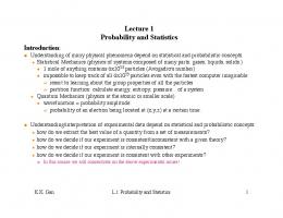
l Understanding of many physical phenomena depend on statistical and ... L1:
Probability and Statistics. 2. Definition of probability: l Suppose we have N trials ...
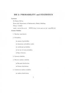
ISE 2: PROBABILITY and STATISTICS. Lecturer. Dr Emma McCoy,. Room 522,
Department of Mathematics, Huxley Building. Phone: X 48553.
There is a 50% chance that the influx (and thus an increase in population) occurs
.... be software or home-made: we could write the numbers on pieces of paper, ....
(This, and the next part of the question are exercises in organizing the list:.
John E. Freund's Mathematical Statistics by Irwin Miller and Marylees Miller, 8th
Edition. Pearson /Prentice Hall Publishers. Methods by which student learning ...
Reading: DeGroot and Schervish “Probability and Statistics”. (4rd Edition) ...
Psycology and Probability: How do people determine expectations? Reading: ...
Chapter 4 Probability and Statistics Probability and Statistics
Chapter 4. Probability and. Statistics. Figliola and Beasley, (1999) ..... 10. Values
for 2 α χ. Goodness of Fit Test. ◇ We can use a chi-squared test to determine ...
Chapter 4 Probability and Statistics
Figliola and Beasley, (1999)
Probability and Statistics Engineering measurements taken repeatedly under seemingly ideal conditions will normally show variability. Measurement system – Resolution – Repeatability
Measurement procedure and technique – Repeatability
Probability and Statistics Measured variable – Temporal variation – Spatial variation
We want: 1. A single representative value that best characterizes the average of the data set. 2. A measure of the variation in a measured data set.
1
True Value True value is represented by
X ' = X ± ux
X = most probable estimate of X’
ux = confidence interval at probability P% which is based on estimates of precision and bias error.
Probability Density Function Central Tendency – says that there is one central value about which all other values tend to be scattered. Probability Density – the frequency with which the measured variable takes on a value within a given interval. The region where observations tend to gather is around the central value.
Plotting Histograms The abscissa is divided in K small intervals between the minimum and maximum values. The abscissa will be divided between the maximum and minimum measured values of x into K small intervals. Let the number of times, nj, that a measured value assumes a value within an interval defined by x-δx ≤ x < x+δx be plotted on the ordinate. For small N, K should be chosen so that nj ≥ 5 for at least one interval.
2
Plotting Histograms For N>40 ; K=1.87(N-1)0.40+1 The histogram displays the tendency and density. If the y-axis is normalized by dividing nj/N, a frequency distribution results.
K=1.87(N-1)0.40+1=7 Cell range: min = 0.68 ; max = 1.34
2δx = (1.34-0.68)/7 = 0.10 x-δx ≤ x < x+δx Cell = 2*δx = 0.10 Note: total frequency equals 100% Note: total occurrence equals N
Probability Density Function P(x) comes from the frequency distribution P( x ) = lim ( nj ) / ( N ( 2δx )) N → ∞ ,δx → 0
- Defines the probability that a measured variable might assume a particular value on any given observation, and also provides the central tendency - The shape depends on the variable in consideration and its natural circumstances/processes. - Plot histograms – compare to common distribution and then fit the parameter. - Unifit is a good PC-based distribution fitting software.
3
Infinite Statistics The most common distribution is the normal or Gaussian distribution. This predicts that the distribution will be evenly distributed around the central tendency. (“bell curve”) The operating conditions that are held fixed are length, temperature, pressure, and velocity.
Gaussian Distribution Pdf for Gaussian: p( x) = 1 / ( v(2 π )1/ 2 exp [( − 1 / 2)(( x − x') 2 / σ 2)]
x’= true mean of x ; σ2 = true variance of x To find/predict the probability that a future measurement falls within some interval. Probability P(x) is the area under the curve between X’±δx on p(x)
4
Gaussian Distribution Simplification of integration: x ' + δx
P( x '− δx≤ x≤ x '+ δx )= ∫ x ' − δx p( x )dx
P(x)=probability p(x)=Pdf
if z1=(x1-x’)/σ and β=(x-x’)/σ dx=σdβ and P( − z1 ≤ β ≤ z1) = 1 / ( 2π )1 / 2 ∫
z1 − e − z1
β2 / 2
dβ
β=standardized normal variant ; z1=interval on p(x)
Table 4.3 Solutions given for this in table 4.3 For z=1, 68.27% of observations within 1 standard deviation of x’ For z=2, 95.45% For z=3, 99.73% The values of z in table 4.3 can be used to predict probability of a unique value occurring in an infinite data set.