Chapter 5 Web Hosting Service Level Agreements - Mathematics in ...

Chapter 5 Web Hosting Service Level Agreements Alan King (Mentor)1 , Mehmet Begen2 , Monica Cojocaru3 , Ellen Fowler2 , Yashar Ganjali4 , Judy Lai5 , Taejin Lee6 , Carmeliza Navasca7 , Daniel Ryan2 Report prepared by Alan King.

5.1

Introduction

This paper proposes a model for a relatively simple Web hosting provider. The model assumes the existence of a load-dispatcher and a finite number of Web-servers. We quantify the quality of service towards the clients of this facility based on a service level agreement between the two parts: the web hosting provider and the client. We assume that the client has the knowledge and resources to quantify its needs. Based on these quantifications, which in our model become parameters, the provider can establish a service offer. In our model, this offer covers the quality of service and the price options for it. The paper is organized as follows: in Section 2 there is a description of the parameters requested from the client and the provider’s offers. In Section 3 we present the mathematical formulation of the model and its dynamics. In Section 4 we introduce an algorithm for the provider’s resource allocation of Web servers in order to optimally serve potential clients, within the quality of service stated. The algorithm, consistent with the provider’s offer, assures substantial profits serving clients requesting a bigger volume of data transfer. Section 5 is an outline of proposed future developments of this model. 1

IBM Thomas J. Watson Research Center University of British Columbia 3 Jeffery Hall, 229 Queen’s University, Canada 4 University of Waterloo 5 University of Texas, Austin 6 Kangwon National University & APCTP, Korea 7 University of California at Davis

2

65

66

CHAPTER 5. WEB HOSTING SERVICE

5.2

Service Level Agreement

In this section we describe a possible agreement between the provider and the clients. We assume that the provider as well as the customer are classifying the requests in classes depending on the file size. Each class will therefore have a different service time. The customers are requested to quantify specific values for the following three parameters for the requests they experience: • estimates, on average, of the arrival rate of file sizes • probability distribution of file sizes • probability distribution of service times With these quantifications/parameters, the provider’s offer includes 1. Base Service Level L represents the base service, the maximum number of servers L to be allocated to a specific class of requests based on the parameters offered by the client. 2. Per-Unit Bid B represents the variable rate the client agrees to pay for adding servers beyond Base Service Level. This might happen if its number of requests increases beyond the estimated level covered in (1). Service up to the Base Service Level L is guaranteed. Requests that exceed L are satisfied if possible when the per-unit bid equals or exceeds the spot market price. Per-Unit Bid can equal 0 or the host’s minimum variable charge M (i.e. cost + economic profit). In other cases the bid is an explicit customer-supplied and changeable bid B, B ≥ M . Whether the bid is 0, M , or B, it reflects the nature of the customer: • the customer wants no service beyond its base level; its implicit bid is 0 • the customer wants service beyond its base level; its implicit bid is M • the customer wants requests beyond its base level to be completed; its explicit bid is B. 3. Quality of Service (level z, probability α ) is denoted by (QoS) and is defined in terms of response time RT by modelling the probability that requests are completed within a specified service time z P [RT > z] < α. The number α is a probability level.

5.3

Dynamics

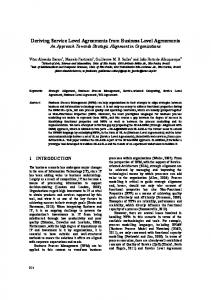
Due to the complexity of the problem, we apply queuing approximations from [4]. Let k = 1, . . . , K index the distinct service classes, and j = 1, . . . , J index the customers. Each class will have a Service Level Agreement, i. e. the parameters identified in the first section will all be indexed by k. The system is composed of an incoming stream of requests with a known Poisson (j) distribution with parameter λk . There are i = 1, . . . , I servers and service time is exponential (j) with parameter 1/µik . See figure below.

π

5.3. DYNAMICS

(1) λk

-

67

'$

Web servers

-

@ @ &% @ '$ @

-

'$

(2)

λk

R @

&%

-

queue

'

-&

&% µ ¡ ¡ q ¡ q ¡ q ¡ '$ (j) ¡ λk ¡ -

$ y y y y y y y y y %

¢ ¢ ¢ ¢ ¡ µ ¢¡ ¡ ¢ @ A A@ A @ R A A A

¢¸

y y

A

y

y

y

&% q q q

(1)

u2i1k

µik-

(2)

y

u2i2k

µik-

-

y UA

y

y

q q 2 q uijk

y y

y

y y

yµik(j)

critical q server

read file size

q

Figure 1: The figure describes the flow of requests with several web servers. All the accepted requests are completely served (i.e. no delay occurs between the moment the request is processed by the server until its final destination). The server is in critical phase if the QoS is low. The probability of the RT is above the bound α.

The available servers are partitioned between the customers so that ∪Jj=1 Ij = I. There are also control actions available to allocate arriving sessions from customer j class k to a given machine i, and also to set the fraction of machine i assigned to the work in progress. Let us call the first control rate u1ijk and the second rate u2ijk . It is assumed that controls are applied randomly to the arrival streams. We have X (j) for k = 1, . . . , K j = 1, . . . , J u1ijk = λk i∈Ij

and

X

(j)

u2ijk = µik

for i ∈ Ij

j = 1, . . . , J

k

Following the analysis in [4], one may estimate the tail probability for response time for each class k customer j and machine i as follows: 2

(j)

1

P [RTik > zjk ] ≤ e−[uijk −uijk ]zjk

(5.1)

To bound the response time it is sufficient to bound the estimate. For planning purposes we will assume that the QoS is violated on a given machine i when the estimate is larger than αjk . In short, we assume the following general framework 1

π

68

CHAPTER 5. WEB HOSTING SERVICE 1. In each interval of time, the number of new requests considered for service is variable and (j) distributed according to a Poisson process with parameter λk . 2. The assignment of rates occurs at the starting point of each time unit. 3. Unserved requests have no impact on the system. (j)

(j)

4. It is possible to forecast the demands λk and the service rates µi,k so that one can allocate processors in time to satisfy the QoS.

5.4

Server Allocation With Delay (SAWD)

At times, it will be necessary to reallocate servers to compensate for predicted abnormal situations. In order to do this, we will have to consider the revenue implications of such a move. By a family of servers we mean a set of servers sharing the load of one Web site. When the number of requests for a Web site causes the probability of a large response time to the customer, we say the family of servers is going red or enters a critical phase. See figure above. To complicate matters, it is not possible to reallocate a server instantaneously. This is due to security issues. To reallocate a server, we must first let its active threads die out. Only then can it be reallocated to a new customer (this usually takes about 5 minutes). Finding an optimal solution through dynamic programming is an extremely difficult task due to the long-time horizon in this problem (24 hours), and the short intervals on which decisions are made. This leads to a problem of such large magnitude that a solution is impractical. Instead, various threshold algorithms can be used to get good solutions. We give an example of such a scheme below. We will make our decisions based on three important values, namely • the probability of a server family going red, P • the expected cost rate incurred from going red and not meeting the SLA, denoted C • the expected revenue rate for providing service beyond the customer’s required level (detailed in their SLA), denoted R (this value may be zero for customers not willing to bid, see Section 2). Note that C and R are both non-negative values and cannot be both zero at the same time for a particular family of servers. This is because C is non-zero when we have gone red as a result of not providing the resources required in the SLA, whereas R is non-zero when we have gone red as a result of traffic being so high that the level of resources agreed to in the SLA is insufficient. As mentioned above, it takes about 5 minutes for a server being moved to come on-line in its new family. However, the server does not immediately stop contributing to its original family. We have approximated that it continues to work for approximately 1/3 of a 5-minute interval (indicating the time period in which it is still handling active threads), after which it is removed

π

5.4. SERVER ALLOCATION WITH DELAY (SAWD)

69

from its family. So, for 2/3 of a 5-minute interval, it is not active in any family. This reflects the period in which it is shutting down and being rebooted. We will introduce subscripts to reflect when a parameter is measured. A subscript of 1 indicates the parameter is measured 5 minutes from now, a subscript of 2 indicates 10 minutes from now, etc. We will introduce a superscript of +1 or -1 to our parameter P to indicate the probability of going red given the addition or subtraction of a server from the family, respectively, i.e. P1−1 indicates the probability of going red 5 minutes from now given that we have removed a server from the family. For each family of servers, we have created the following measures: N eed = P1 · C1 + P2 · C2 + (1 − P1+1 )R1 + (1 − P2+1 )R2

(5.2)

Note that due to the mutually non-zero relationship of C and R mentioned above, either the first two terms above are zero, or the second two terms are zero. If the first two terms are zero, this indicates that a traffic level higher than agreed to in the SLA would push us into red, and if the last two terms are zero, this indicates that we might fall into a penalty situation. Thus, N eed can reflect either a possibility to make extra revenue (if action is taken), or the possibility of paying penalties (if action is not taken), depending on which terms are zero. The higher the N eed of a family is, the more money that can be lost or earned by adding a server to that family. Availability =

(5.3)

2 −1 2 · C1/3 + P1−1 · C1 + P2−1 · C2 + (1 − P1/3 )R1/3 + = [ P1/3 3 3 (1 − P1 )R1 + (1 − P2 )R2 Availabiliy is closely related to N eed, but there are two significant differences. The first is that the superscripts reflect that we are considering removing a computer from the family, as opposed to adding one. The second difference is that there are two extra terms. These terms reflect the fact that the server will be removed from the family after 1/3 of the first 5 minute interval. Availability is intended to measure the amount of penalties that will be paid, or revenue lost if we move a server from that family. Hence, the smaller the Availability of a family is, the less money we are likely to lose from moving a server from that family. Note that all terms in the above equations are non-negative, and for one particular family of servers, the Availability value will always exceed the N eed value. In order to decide when to take action and move a server from one family to another, we use the following heuristic: 1. Calculate the N eed and Availability for every family of servers. 2. Compare the largest N eed value with the smallest Availability value. If the N eed value exceeds the Availability value, one server is taken from the family corresponding to the Availability value and given to the family corresponding to the N eed value. 3. If a server was told to move, go back to step 1 (note: the probabilities will change as the number of servers used to make the calculations will be different). Terminate the loop if no server was told to move in the last iteration.

π

70

CHAPTER 5. WEB HOSTING SERVICE

The above iteration loop should be performed on a frequent basis. We suggest about every 15 seconds. This is only one possible heuristic, and we have yet to actually compare it in simulation with an optimal solution. However, it has the obvious advantage of requiring considerably less computation than a long-time horizon dynamic program, which allows it to be performed very often. This allows us to react nearly instantaneously to a predicted critical situation. The P , C and R values are obtained from forecasts provided from the router control level.

5.5

Future Work

We would like to extend the single server single queue dynamics to a system which encompasses the initiation of the SAWD. Quantifying the QoS was the challenging task during the allotted time; thus we must decide which measurement of the QoS best fits the model. In consequence, expressing the measure of QoS is imperative in the formulation of the stochastic optimal control problem for maximizing the total expected revenue. Finding a fair price is another goal. In addition, we wish to perform simulations to test the heuristics and investigate the distribution of the real file size data.

π

Bibliography [1] Bertsekas, D., Dynamic Programming and Stochastic Control, New York: Academic Press, 1976. [2] Chang, Y-C., Guo, X., Kimbrel, T. and King, A., Optimal allocation policies for Web hosting, IBM T.J. Watson Research Centre, P.O. Box 704, N.Y. 10598. [3] Chatwin, R. E., Continuous time airline overbooking with time dependent fares and refunds, Applied Decision Analysis LLC, Transportation Science, 33(2), (1999), 182-199. [4] Liu, Z. et al., On maximizing service level agreement profits, IBM T.J. Watson Research Center, P.O.Box 704, NY 10598. [5] Nortel and Bay Networks, IP QoS-A bold new network, September 1998, Nortel Marketing Publications, Dept. 4262, P.O. Box 13010, Research Triangle Park, NC 27709. [6] Paschalidis, I. Ch. and Tsitsiklis, J.N., Congestion-depending pricing of network services, Technical Report, October 1998, Dept. of Manufacturing Engineering, Boston University, Boston MA 02215. [7] Subramaanian, J., Stidham, S. and Lautenbacher, C.J., Airline yield management with overbooking, cancellation, and no-shows, Transportation Science 33(2), (1999), 147-167.

71