San Mateo, California. Morgan Kauffman Publishers. Coello, C. A. C. (1999). A Comprehensive Survey of Evolutionary-Based. Multiobjective Optimization ...
Chapter 7 ASSESSMENT METHODOLOGIES FOR MULTIOBJECTIVE EVOLUTIONARY ALGORITHMS Ruhul Sarker and Carlos A. Coello Coello Abstract
The Pareto-based evolutionary multiobjective algorithms have shown some success in solving multiobjective optimization problems. However, it is difficult to judge the performance of multiobjective algorithms because there is no universally accepted definition of optimum in multiobjective as in single-objective optimization problems. As appeared in the literature, there are several methods to compare two or more multiobjective algorithms. In this chapter, we discuss the existing comparison methods with their strengths and weaknesses.
Keywords: multiobjective, Pareto front, metrics, evolutionary algorithm, performance assessment
1.
Introduction
In multiobjective optimization problems, we define the vector-valued objective function f : Rn → Rm where m > 1, n is the dimension of the decision vector, x, and m is the dimension of the objective vector, y. For the case of minimization problems, we intend to minimize y = f (x) = (f1 (x), · · · , fm (x)), where x ∈ Rn , and y ∈ Rm . A solution ya is said to dominate solution yb if yai ≤ ybi , ∀i ∈ {1, · · · , m} and yai < ybi , ∃i ∈ {1, · · · , m}. In most cases, the objective functions are in conflict, because in order to decrease any of the objective functions, we need to increase other objective functions. When we have a solution which is not dominated by any other solution in the feasible space, we call it Pareto-optimal.
177
178
EVOLUTIONARY OPTIMIZATION
The set of all Pareto-optimal solutions is termed the Pareto-optimal set, efficient set or admissible set. Their corresponding objective vectors are called the nondominated set. Fonseca and Fleming (1995), categorized the evolutionary based techniques for multiobjective optimization into three approaches: plain aggregating approaches, population-based non-Pareto approaches, and Pareto-based approaches. A comprehensive survey of the different techniques under these three categories can be found in Coello (1999), in Veldhuizen (1999) and in the last two chapters of this book. In multiobjective optimization, determining the quality of solutions produced by different evolutionary algorithms is a serious problem for researchers because there is no well accepted procedure in the literature. The problem is certainly difficult due to the fact that, unlike single-objective optimization, in this case we need to compare vectors (representing sets of solutions). The chapter is organized as follows. We will start by surveying the most important work on performance assessment methodologies reported in the specialized literature, describing each proposal and analyzing some of their drawbacks. Then, we will present a brief comparative study of the main metrics discussed and we will conclude with some possible paths of future research in this area.
2.
Assessment Methodologies
The definition of reliable assessment methodologies is very important to be able to validate an algorithm. However, when dealing with multiobjective optimization problems, there are several reasons why the assessment of results becomes difficult. The initial problem is that we will be generating several solutions, instead of only one (we aim to generate as many elements as possible of the Pareto optimal set). The second problem is that the stochastic nature of evolutionary algorithms makes it necessary to perform several runs to assess their performance. Thus, our results have to be validated using statistical analysis tools. Finally, we may be interested in measuring different things. For example, we may be interested in having a robust algorithm that approximates the global Pareto front of a problem consistently, rather than an algorithm that converges to the global Pareto front but only occasionally. Also, we may be interested in analyzing the behavior of an evolutionary algorithm during the evolutionary process, trying to establish its capabilities to keep diversity and to progressively converge to a set of solutions close to the global Pareto front of a problem.
Assessment Methodologies for MEAs
179
The previous discussion is a clear indication that the design of metrics for multiobjective optimization is not easy. The next topic to discuss is what to measure. It is very important to establish what sort of results we expect to measure from an algorithm so that we can define appropriate metrics. Three are normally the issues to take into consideration to design a good metric in this domain (Zitzler et al., 2000): 1 Minimize the distance of the Pareto front produced by our algorithm with respect to the global Pareto front (assuming we know its location). 2 Maximize the spread of solutions found, so that we can have a distribution of vectors as smooth and uniform as possible. 3 Maximize the number of elements of the Pareto optimal set found. Next, we will review some of the main proposals reported in the literature that attempt to capture these three issues indicated above. As we will see, none of these proposals really captures the three issues in a single value. In fact, to attempt to produce a single metric that captures these three issues may prove fruitless, since each of these issues refers to different performance aspects of an algorithm. Therefore, their fusion into a single value may be misleading. Interestingly, the issue of designing a good assessment measure for this domain is also a multiobjective optimization problem. The techniques that have attempted to produce a single value to measure the three issues previously discussed, are really some form of an aggregating function and therefore the problems associated with them (Coello, 1999). It is therefore, more appropriate to use different metrics to evaluate different performance aspects of an algorithm.
2.1
A Short Survey of Metrics
As we will see in our following survey of metrics, most of the current proposals assume that the global Pareto front (P Fglobal ) of the multiobjective optimization under study is known or it can be generated (e.g., through an enumerative approach). If that is the case, we can test the performance of a multiobjective evolutionary algorithm (MEA) by comparing the Pareto fronts produced by our algorithm (P Fobtain ) against the global Pareto front (P Fglobal 1 ) and then determine certain error measures that indicate how effective is 1 We
have adopted a notation similar to the one proposed by Veldhuizen (Veldhuizen, 1999).
180
EVOLUTIONARY OPTIMIZATION
the algorithm analyzed. The error rate and generational distance metrics discussed next make this assumption.
2.1.1 Error Rate. This metric was proposed by Veldhuizen (1999) to indicate the percentage of solutions (from P Fobtain ) that are not members of P Fglobal : �n ER =
i=1 ei
n
,
(7.1)
where n is the number of vectors in P Fobtain ; ei = 0 if vector i is a member of P Fglobal , and ei = 1 otherwise. It should then be clear that ER = 0 indicates an ideal behavior, since it would mean that all the vectors generated by our MEA belong to P Fglobal . Note that this metric requires knowing the number of elements of the global Pareto optimal set, which is often impossible to determine. Veldhuizen and Lamont (1998,1999) have used parallel processing techniques to enumerate the entire intrinsic search space of an evolutionary algorithm, so that P Fglobal can be found. However, they only reported success with strings of ≤ 26 bits. To enumerate the entire intrinsic search space of realworld multiobjective optimization problems with high dimensionality is way beyond the processing capabilities of any computer (otherwise, any multiobjective optimization problem could be solved by enumeration). This metric clearly addresses the third of the issues discussed in Section 2.
2.1.2 Generational Distance. The concept of generational distance (GD) was introduced by Veldhuizen and Lamont (1998) as a way of estimating how far are the elements in P Fobtain from those in P Fglobal and is defined as: �� n GD =
2 i=1 di
n
(7.2)
where n is the number of vectors in P Fobtain and di is the Euclidean distance (measured in objective space) between each of these and the nearest member of P Fglobal . It should be clear that a value of GD = 0 indicates that all the elements generated are in P Fglobal . Therefore, any other value will indicate how “far” we are from the global Pareto front of our problem. Similar metrics were proposed by Rudolph (1998), Schott (1995), and Zitzler et al. (2000). This metric also refers to the third issue discussed in Section 2
181
Assessment Methodologies for MEAs
2.1.3 Spread. The spread measuring techniques measure the distribution of individuals in P Fobtain over the nondominated region. For example, Srinivas and Deb (1994) proposed the use a chi-squared distribution: � � q+1 � �� ni − n ¯i 2 � SP = (7.3) σi i=1
where: q is the number of desired (Pareto) optimal points (it is assumed that the (q +1)-th subregion is dominated by the q-th subregion), ni is the number of individuals in the i-th niche (or subregion (Deb and Goldberg, 1989)) of the nondominated region, n ¯ i is the expected number of individuals present in the i-th niche, and σi2 is the variance of the individuals present in the i-th subregion of the nondominated region. Deb (1989) had previously used probability theory to estimate that: n ¯i ), i = 1, 2, ...., q, (7.4) P where P is the population size. Since the (q + 1)-th subregion is a dominated region, then n ¯ q+1 = 0 (i.e., we do not want to have any individuals in that region). Also, Deb’s study showed that: ¯ i (1 − σi 2 = n
2 = σq+1
q �
σi2
(7.5)
i=1
Then, if SP=0, it means that our MEA has achieved an ideal distribution of points. Therefore, low values of SP imply a good distribution capacity of a given MEA. To analyze the distribution using this measure, the nondominated region is divided into a certain number of equal subregions (this number is given by the decision maker). Knowing the population size used by the MEA under study, we can compute the amount of expected individuals in each subregion. This value is then used to compute the deviation measure indicated above. A similar metric, called “efficient set spacing” (ESS) was proposed by Schott (1995): � � e � 1 �
�2 � (7.6) d¯ − di ESS = e−1 i=1
182
EVOLUTIONARY OPTIMIZATION
where:
j j i i di = minj |f1 − f1 | + |f2 − f2 |
(7.7)
where: j = 1, . . . , e, and d¯ refers to the mean of all di and e is the number of elements of the Pareto optimal set found so far. If ESS = 0, then it means that our MEA is giving us an ideal distribution of the elements of our nondominated vectors. Schott’s approach is based on a Holder metric of degree one (Horn and Nafpliotis, 1993) and measures the variance of the distance of each member of the Pareto optimal set (found so far) with respect to its closest neighbor. Note, however, that, as indicated by Veldhuizen (1999), this metric has to be adapted to consider certain special cases (e.g., disjoint Pareto fronts), and it may also be misleading unless it is combined with a metric that indicates the number of elements of the global Pareto optimal set found (e.g., if we produce only two solutions, this metric would indicate an ideal distribution). Although none of these spread metrics really requires that we know P Fglobal , they both implicitly assume that our MEA has converged to global nondominated solutions. Otherwise, knowing that our algorithm produces a good distribution of solutions may become useless. It should be clear that these metrics refer to the second issue discussed in Section 2
2.1.4 Space Covered. Zitzler and Thiele (1999) proposed a similar metric called “Size of the Space Covered” (SSC). This metric estimates the size of the global dominated set in objective space. The main idea behind this metric is to compute the area of objective function space covered by the nondominated vectors that our MEA has generated. For biobjective problems, each dominated vector represents a rectangle defined by the points (0,0) and (f1 (xi ), f2 (xi )), where f1 (xi ) and f2 (xi ) are nondominated solutions. Therefore, SSC is computed as the union of the areas of all the rectangles that correspond to the nondominated vectors generated. However, the main drawback of this metric is that it may be misleading when the shape of the Pareto front is non-convex (Zitzler and Thiele, 1999). Laumanns et al. (1999), used the concept of space coverage for comparing problems with more than two objectives. In their paper, they considered an m-dimensional cuboid as a reference set, from which the MEA under investigation should cover the maximum possible dominated space. Every nondominated solution gives a cone of dominated solutions. The intersection of this cone with the reference cuboid (which is also a
Assessment Methodologies for MEAs
183
cuboid) adds to the dominated volume. In calculating the dominated volume, the overlapping parts of different solutions are not counted multiple times. In this method, the reference cuboid is developed using the single objective optimal solutions. That means the single objective optimal solution must be either known or computed before judging the quality of a MEA. If the single objective solutions are not known, for a problem with m functions, one has to solve m single objective problems to generate the reference cuboid. Potentially, this could be a expensive process (computationally speaking), particularly when dealing with real-world applications. The value of space coverage varies with the number of nondominated solution points and their distribution over the Pareto front. We can then see that this metric tries to combine into a single value the three issues discussed in Section 2 Therefore, as indicated by Zitzler et al. (2000) the metric will be ineffective in those cases in which two algorithms differ in more than one of these three criteria previously mentioned (i.e., distance, spread and number of elements of the global Pareto optimal set found). That is why Veldhuizen (1999) suggested to use a ratio instead, but his metric also assumes knowledge of P Fglobal .
2.1.5 Coverage Metric. Zitzler and Thiele (1999) proposed another metric for comparing the performances of different MEAs. In this case, two nondominated sets are compared calculating the fraction of each of them that is “covered” (or dominated) by the other one. Suppose there are two algorithms A1 and A2 to compare their performances. In this method, the resulting set of nondominated points from a single run of algorithm A1 and another from a single run of algorithm A2 are processed to yield two numbers: the percentage of points from algorithm A1 which are equal to or dominated by points from A2, and vice versa. Statistical tests can be performed on the numbers yielded from several such pairwise comparisons. Let X � , X �� ⊆ X be two sets of decision vectors. The function CM maps the ordered pair (X � , X �� ) to the interval [0,1] (Zitzler and Thiele, 1999): CM (X � , X �� ) =
| {a�� ∈ X �� ; a� ∈ X � : a� � a�� } | | X �� |
If CM (X � , X �� ) = 1, then it means that all points in X �� are dominated by or are equal to points in X � . If CM (X � , X �� ) = 0, then it means that none of the points in X �� are covered by the set X � . This method can be used to show whether the outcomes of one algorithm dominate the outcomes of another algorithm without indicating
184
EVOLUTIONARY OPTIMIZATION
how much better it is. Also, note that this comparison technique does not check the uniformity of solution points along the trade-off surface. Another problem with this approach is that it may return a better value for an algorithm that produces a single vector, closer to the global Pareto optimal front than for another algorithm that produces several well-distributed vectors that are, however, farther from the global Pareto optimal front (Knowles and Corne, 2000). This metric only refers to the first issue discussed in Section 2 In fact, this metric is meant to complement the Space Covered metric previously discussed (Zitzler and Thiele, 1999). In his dissertation, Zitzler (1999) proposed another metric called “Coverage difference of two sets”, that solves some of the problems of the Coverage Metric.
2.1.6 Statistical Comparison. MEAs are usually run several times to end up with a set of alternative solutions for MOPs from which the decision maker has to choose one. So, when we compare different MEAs, it is logical to compare them statistically instead of comparing only scalar values as in the single objective case. An statistical comparison method called “attainment surfaces” was introduced by Fonseca and Fleming (1996). Consider the approximations to the Pareto optimal front for two algorithms A1 and A2 as shown in Figure 7.1. The lines joining the points (solid for A1 and dashed for A2) indicate the so-called attainment surfaces. An attainment surface divides objective space into two regions: one containing vectors which are dominated by the results produced by the algorithm, and another one that contains vectors that dominate the results produced by the algorithm. As shown in Figure 7.1, a number of sampling lines (L1, L2, ) can be drawn from the origin, which intersect the attainment surfaces, across the full range of the Pareto front (trade-off surfaces obtained). The range of the Pareto surface is usually specified by the decision maker. For a given sampling line, the intersection of an algorithm closer to the origin (assuming minimization for both objectives) is the winner. In our case, algorithm A1 is winner for line L3 and A2 is winner for line L4. Fonseca and Fleming’s idea was to consider a collection of sampling lines which intersect the attainment surfaces across the full range of the Pareto frontier. If MEAs are run r times, each algorithm will return r attainment surfaces, one from each run. Having these r attainment surfaces, some from algorithm A1 and some from algorithm A2, a single sampling line yields r points of intersection, one for each surface. These intersections form a univariate distribution, and therefore, we can perform standard non-parametric statistical procedures to determine whether or not the
185
Assessment Methodologies for MEAs
A2 A1
L1 L2 L3
f2
L4 A2
L5 L6 L7
A1
f1
Figure 7.1.
Sampling the Pareto frontier using lines of intersection
intersections for one of the algorithms occurs closer to the origin with some statistical significance. Such statistical tests have been performed by (Knowles and Corne, 2000) for each of several lines covering the Pareto tradeoff area. Insofar as the lines provide a uniform sampling of the Pareto surface, the result of this analysis yields two numbers—a percentage of the surface in which algorithm A1 outperforms algorithm A2 with statistical significance, and that when algorithm A2 outperforms algorithm A1. Knowles and Corne (2000) presented their results of a comparison in the form of a pair [a1,a2], where a1 gives the percentage of the space (i.e. the percentage of lines) on which algorithm A1 was found statistically superior to A2, and a2 gives the similar percentage for algorithm A2. Typically, if both A1 and A2 are ‘good’, then a1 + a2 ¡ 100. The quantity [100 - (a1 + a2)], of course, gives the percentage of the space on which the results were statistically inconclusive. They use statistical significance at the 95 percent confidence level. Knowles and Corne (2000) also extended their comparison methodology for comparing more than two algorithms. If the algorithms are competitive, the results may vary with the number of sampling lines drawn since the procedure considers only the intersection points of sampling lines and attainment surfaces. Knowles and Corne (2000) proposed that 100 lines must be adequate, although, obviously, more lines the better. They have shown experimentally that
186
EVOLUTIONARY OPTIMIZATION
the percentage of the space (a1 + a2) increases, to give statistically significant results, with the increased number of lines. A drawback of this approach is that it remains unclear how much better is one algorithm from another one against which it is being compared (Zitzler, 1999). An important aspect of this metric, however, is that the global Pareto optimal set does not need to be known. Note that this metric is similar to the Coverage Metric, since they both compare the outcomes of two algorithms but none allows to determine how much better is an algorithm compared to others. This metric is also addressing only the first of the issues discussed in Section 2 In more recent work, da Fonseca et al. (2001) extended their original proposal relating their attainment function definition to random closed set theory (Matheron, 1975). Under this scheme, the attainment function can be seen as a generalization of the multivariate cumulative distribution function. The metric, in fact, addresses the three issues discussed in Section 2 However, its main drawback is that computing the multivariate empirical cumulative distribution function may be quite difficult and very expensive (computationally speaking) (da Fonseca et al., 2001).
3.
Discussion
In practice, P Fglobal is a collection of points on the global Pareto front. To make metrics such as the Error Rate (ER) and Generational Distance (GD) meaningful, we must have a large number of points without any gap so that the global Pareto front looks like a continuous line instead of a dotted line. Suppose that we have two algorithms (A1 and A2) to compare with respect to P Fglobal . Algorithm A1 produces only a few alternative solutions and all of these solutions are scattered and are members of P Fglobal , then ER (and GD) being zero indicates that the algorithm produces perfect results. Algorithm A2 produces many alternative but evenly distributed solutions. The ER (same for GD) value of A2 is greater than zero since there are few points who are not members of P Fglobal . Should we say A1 is better than A2? In a multiobjective decision process, more alternative solutions mean more flexibility to the human decision maker. Though the Error Rate and Generational Distance for A1 are zero, the number of alternative solutions and their distributions are not favorable for a good decision making process. So, it should be clear that ER and GD are not sufficient to judge the performance of MEAs. The Error Rate and Generational Distance can be used, when the Pareto fronts are known, to get an indication of errors involved with the
Assessment Methodologies for MEAs
187
obtained front. However, for an unsolved problem, it is impossible to know its Pareto front beforehand. The Spread metric may help to judge an algorithm when the global Pareto front is unknown (although, this metric implicitly assumes that convergence to the global Pareto front has been achieved). However, it only judges the uniformity of solution points over different subregions without indicating the overall quality of solutions. The Space Covered metric shows the dominated space covered by the solutions obtained from an algorithm. This metric, however, may be misleading when the Pareto front of the problem is concave. The Coverage M etric shows whether the outcomes of one algorithm dominate the outcomes of another algorithm without indicating how much better it is. This comparison technique does not check the uniformity of solution points along the Pareto trade-off surface. Therefore, this metric will be misleading when algorithm A1 produces only one vector that is closer to the global Pareto front of the problem than the solutions produced by algorithm A2, which are uniformly distributed but are dominated by the solutions of A1. The Statistical Comparison technique seems to be reasonably good in comparing different MEAs though the results may vary with the number of sampling lines. In contrast to other methods, this method is judging the overall quality of Pareto trade-off surface based on the sample information (taking only points on the intersection of attainment surfaces and sampling lines). In addition it does not explicitly measure the uniformity of the solutions points. Nevertheless, this metric is also incapable of establishing how much better is a certain algorithm with respect to others. As discussed earlier, decision makers are interested in a good number of uniformly distributed solution points on the trade-off surface along their relative optimality. By the term relative optimality for a two objective minimization problem, we mean, the solution points (when plotted one objective versus the other) must be as close to the origin (0,0) as possible in a given subregion. No comparison technique gives a clear indication about the relative performance of an algorithm. However a combination of a few techniques and some other simple considerations may help to compare two or more algorithms up to a certain level. The first thing is to plot the Pareto fronts and inspect visually their relative locations, relative number of points in each front and their distribution. The visual inspection is acceptable when one algorithm clearly outperforms the other. This method is limited to two or three function problems only. When the algorithms are very competitive, the statistical comparison along with the space covered, number of solution points,
188
EVOLUTIONARY OPTIMIZATION
average distance between neighboring points (with their distribution), and average distance between the origin (or any other reference point) and the solution points (with their distribution) may help to compare two or more MEAs. There are other proposals for performance assessment measures in the specialized literature. For example, Zitzler et al. (2000) proposed a family of scale-dependent measures. Esbensen and Kuh (1996) and Ang et al. (2001) proposed the use of a utility function to determine the quality of the solutions produced by a MEA. This metric considers only nearness to the global Pareto optimal front, but not spread or number of elements achieved. Veldhuizen (1999) proposed a multiobjective version of the “progress measure” metric proposed by Thomas B¨ack (1996). In this case, the relative convergence improvement of the MEA is measured. The main drawback of this metric is that it may be misleading in certain situations (e.g., when we find a single vector that belongs to a Pareto front closer to the global Pareto front than those vectors previously found by the algorithm). However, it is important to keep in mind that combining the three issues discussed before is still an open research area, and it currently seems better to apply independently more than one metric to the same problem and analyze the combination of results found. Notice also that some specific domains may allow the definition of more precise metrics. Such is the case of multiobjective combinatorial optimization, in which several quality measures have been proposed (see for example (Jaszkiewicz et al., 2001; Carlyle et al., 2001)).
4.
Comparing Two Algorithms: An Example
In evolutionary computation, when comparing two algorithms, it is considered common practice that they both have the same representation (e.g., binary), operators (i.e., crossover and mutation), and parameters (i.e., crossover and mutation rates, population size, etc.) on all the functions to be tested. Otherwise, the comparison is not considered fair. For example, the comparison between an algorithm AL1 with binary representation (with one-point crossover and bit-flip mutation) and another algorithm AL2 with real number representation (with Gaussian mutation) would be treated as an improper comparison even if they both use the same parameters. If different parameters are used (e.g., different population sizes), it may become obvious to anyone that the amount of fitness function evaluations of the algorithms compared will be different and, therefore, any comparison will be unfair. However, if only the representation and operators are different, it is perhaps not so obvious why
Assessment Methodologies for MEAs
189
the comparison is unfair. The reasons for that assumption are related to the role of the representation and the genetic operators in an evolutionary algorithm (Whitley et al., 1998; Caruana and Schaffer, 1988; Ronald, 1997; Eshelman et al., 1989; Spears and Jong, 1991; Fogarty, 1989). If the representation, operators of two algorithms are same, the superiority of one algorithm over the other really shows the strength of the algorithmic design for the given representation and operators. We must mention here that there is a lot of empirical evidence regarding the fact that the real number representation works better than binary representation for most real valued problems (Michalewicz, 1996). From the optimization point of view, the quality of solutions and computational complexity of the algorithms are only two parameters to be considered when comparing any two algorithms with the same starting solution. If the algorithm AL2 produces better results than AL1 and has a lower computational complexity (i.e., lower computational time), the algorithm AL2 can be considered as the better algorithm irrespective of representation and operators. Of course, one has to test a sufficient number of problems including extreme cases to conclude the quality of an algorithm. In evolutionary algorithms, the same rule can be applied using equal population size as equivalent to same initial solution. In this section, we compare two algorithms of different representations, not to be back to the debate of valid or invalid comparison, but just to demonstrate the assessment methodologies described in this chapter. The two algorithms used in this comparison are: Differential Evolution based Multiobjective Algorithms (Abbass et al., 2001), referred as P DE in this chapter, and Strength Pareto Evolutionary Algorithm (Zitzler and Thiele, 1999), referred as SP EA. SP EA uses binary representation with one-point crossover and bit-flip mutation and P DE uses real number representation with Gaussian mutation. We use only one test problem T 1 from (Abbass et al., 2001) that was also tested by (Zitzler and Thiele, 1999). The first method, reported in this section, is the graphical presentation of function values. The outcomes of the first five runs of the test function from each algorithm were unified. Then the dominated solutions are deleted from the union set, and all the nondominated ones are plotted. The figure is reproduced from (Abbass et al., 2001). As you can see the plot in 7.2, P DE clearly shows superiority over SP EA. From this observation, one may think that P DE is better than SP EA for any or all runs for this test problem. The second comparison method is to measure the coverage of two solution sets produced by the two algorithms. The value of the coverage metric, calculated from 20 runs, of average 98.65 indicates that P DE
190
EVOLUTIONARY OPTIMIZATION
1 0.9 0.8 0.7
F2
0.6 0.5 SPEA 0.4 PDE
0.3 0.2 0.1 0 0
0.1
0.2
Figure 7.2.
0.3
0.4
0.5 F1
0.6
0.7
0.8
0.9
1
Pareto frontier for PDE and SPEA
covers SP EA for most cases, but not for all of them. However, SP EA also covers P DE for a few occasions. That means, P DE is not better than SP EA for all cases. The statistical comparison, using the solutions of 20 runs, shows that [a1,a2] = [84.30, 15.10]. That means, P DE is statistically superior to SP EA for 84.30 percentage of the space (i.e. the percentage of lines) and SP EA is statistically superior to P DE for 15.10 percentage. The quantity [100 - (a1 + a2)] = 0.60, of course, gives the percentage of the space on which the results were statistically inconclusive. We use statistical significance at the 95 percent confidence level and the number of lines equal to 100. For SP EA, the value of statistical comparison metric is better than the coverage metric. Once again, SP EA is not that bad compared to P DE as we thought after visual inspection. The average space coverage by P DE and SP EA are 0.341045 and 0.369344 respectively. The average spacing between the adjacent solution points are 0.1975470 and 0.2447740 for P DE and SP EA respectively. The average distance from the origin to the solution points are 0.6227760 and 0.7378490 for P DE and SP EA respectively. From the above indicators, one can conclude easily that P DE solutions are better than SP EA for the given test problem. Although the amount of computations required by the two algorithms, to solve this
Assessment Methodologies for MEAs
191
test problem, is very much similar (in terms of fitness function evaluations), the P DE algorithm gives special attention to the uniformity of the solution points in each generation (Abbass et al., 2001).
5.
Conclusions and Future Research Paths
In this chapter, we have reviewed some of the most important proposals for metrics found in the literature on evolutionary multiobjective optimization. As we have seen, most of the proposals defined in this context normally consider only one of the three fundamental aspects that we need to measure when dealing with multiobjective optimization problems: closeness to the global Pareto front, spread along the Pareto front or number of elements of the Pareto optimal set found. As mentioned before, several issues still remain as open paths for future research. Consider for example the following: It may be important to consider additional issues such as efficiency (e.g., CPU time or number of fitness function evaluations) in the design of a metric. No current metrics consider efficiency as another factor to be combined with the three issues previously discussed (it tends to be measured independently or to be considered fixed), although in some recent work by Ang et al.(2001), they propose to use a metric proposed by Feng et al. (1998) (called “optimizer overhead”) for that sake. However, this metric also (implicitly) assumes knowledge of the global Pareto front of the problem when dealing with multiple objective optimization problems. Few metrics are really used to measure progress of MEAs through generations. Studies in which such progress is analyzed are necessary to understand better the behavior of MEAs, particularly when dealing with difficult problems. There is a notorious lack of comparative studies in which several metrics and MEAs are used. Such studies would not only indicate strenghts and weaknesses of MEAs, but also of the metrics used to compare them. There are no formal studies that indicate if measuring performance in phenotypic space (the usual norm in evolutionary multiobjective optimization) is better than doing it in genotypic space (as in operations research) (Veldhuizen, 1999). Most researchers tend to use the performance assessment measures found in the literature without any form of analysis that indicates if they are suitable for the technique and/or domain to which they will be applied.
192
EVOLUTIONARY OPTIMIZATION
New metrics are of course necessary, but their type is not necessarily straightforward to determine. Statistical techniques seem very promising (da Fonseca et al., 2001), but other approaches such as the use of hyperareas looks also promising (Zitzler and Thiele, 1999). The real challenge is to produce a metric that allows to combine the three issues previously mentioned (and perhaps some others) in a non-trivial form (we saw the problems when using an aggregating function for this purpose). If such a combination is not possible, then it is necessary to prove it in a formal study and to propose alternatives (i.e., to indicate what independent measures need to be combined to obtain a complete evaluation of a MEA). Publicly-available test functions and results to evaluate multiobjective optimization techniques are required, as some researchers have indicated (Veldhuizen, 1999; Ang et al., 2001). It is important that researchers share the results found in their studies, so that we can build a database of approximations to the Pareto fronts of an important number of test functions (particularly, of real-world problems). The EMOO repository at: http://www.lania.mx/~ccoello /EMOO/ is attempting to collect such information, but more efforts in that direction are still necessary.
Acknowledgments The second author acknowledges support from the mexican Consejo Nacional de Ciencia y Tecnolog´ıa (CONACyT) through project number 34201-A.
References Abbass, H., Sarker, R., and Newton, C. (2001). PDE: A Pareto Frontier Differential Evolution Approach for Multiobjective Optimisation Problems. In Proccedings of the Congress on Evolutionary Computation 2001, pages 971–978. Seoul, Korea. Ang, K., Li, Y., and Tan, K. C. (2001). Multi-Objective Benchmark Functions and Benchmark Studies for Evolutionary Computation. In Proceedings of the International Conference on Computational Intelligence for Modelling Control and Automation (CIMCA’2001), pages 132–139, Las Vegas, Nevada. B¨ack, T. (1996). Evolutionary Algorithms in Theory and Practice. Oxford University Press, New York. Carlyle, W. M., Kim, B., Fowler, J. W., and Gel, E. S. (2001). Comparison of Multiple Objective Genetic Algorithms for Parallel Machine Scheduling Problems. In Zitzler, E., Deb, K., Thiele, L., Coello,
REFERENCES
193
C. A. C., and Corne, D., editors, First International Conference on Evolutionary Multi-Criterion Optimization, pages 472–485. SpringerVerlag. Lecture Notes in Computer Science No. 1993. Caruana, R. and Schaffer, J. D. (1988). Representation and Hidden Bias: Gray vs. Binary Coding for Genetic Algorithms. In Proceedings of the Fifth International Conference on Machine Learning, pages 132–161, San Mateo, California. Morgan Kauffman Publishers. Coello, C. A. C. (1999). A Comprehensive Survey of Evolutionary-Based Multiobjective Optimization Techniques. Knowledge and Information Systems. An International Journal, 1(3):269–308. da Fonseca, V. G., Fonseca, C. M., and Hall, A. O. (2001). Inferential Performance Assessment of Stochastic Optimisers and the Attainment Function. In Zitzler, E., Deb, K., Thiele, L., Coello, C. A. C., and Corne, D., editors, First International Conference on Evolutionary Multi-Criterion Optimization, pages 213–225. Springer-Verlag. Lecture Notes in Computer Science No. 1993. Deb, K. (1989). Genetic Algorithms in Multimodal Function Optimization. Technical Report 89002, The Clearinghouse for Genetic Algorithms, University of Alabama, Tuscaloosa, Alabama. Deb, K. and Goldberg, D. E. (1989). An Investigation of Niche and Species Formation in Genetic Function Optimization. In Schaffer, J. D., editor, Proceedings of the Third International Conference on Genetic Algorithms, pages 42–50, San Mateo, California. George Mason University, Morgan Kaufmann Publishers. Esbensen, H. and Kuh, E. S. (1996). Design space exploration using the genetic algorithm. In IEEE International Symposium on Circuits and Systems (ISCAS’96), pages 500–503, Piscataway, NJ. IEEE. Eshelman, L. J., Caruana, R. A., and Schaffer, J. D. (1989). Biases in the Crossover Landscape. In Schaffer, J. D., editor, Proceedings of the Third International Conference on Genetic Algorithms, pages 10–19, San Mateo, California. Morgan Kaufmann Publishers. Feng, W., Brune, T., Chan, L., Chowdhury, M., Kuek, C., and Li, Y. (1998). Benchmarks for Testing Evolutionary Algorithms. In Proceedings of the Third Assia-Pacific Conference on Control and Measurement, pages 134–138, Dunhuang, China. Fogarty, T. C. (1989). Varying the Probability of Mutation in the Genetic Algorithm. In Schaffer, J. D., editor, Proceedings of the Third International Conference on Genetic Algorithms, pages 104–109, San Mateo, California. Morgan Kaufmann Publishers. Fonseca, C. M. and Fleming, P. J. (1995). An Overview of Evolutionary Algorithms in Multiobjective Optimization. Evolutionary Computation, 3(1):1–16.
194
EVOLUTIONARY OPTIMIZATION
Fonseca, C. M. and Fleming, P. J. (1996). On the Performance Assessment and Comparison of Stochastic Multiobjective Optimizers. In Voigt, H.-M., Ebeling, W., Rechenberg, I., and Schwefel, H.-P., editors, Parallel Problem Solving from Nature—PPSN IV, Lecture Notes in Computer Science, pages 584–593, Berlin, Germany. Springer-Verlag. Horn, J. and Nafpliotis, N. (1993). Multiobjective Optimization using the Niched Pareto Genetic Algorithm. Technical Report IlliGAl Report 93005, University of Illinois at Urbana-Champaign, Urbana, Illinois, USA. Jaszkiewicz, A., Hapke, M., and Kominek, P. (2001). Performance of Multiple Objective Evolutionary Algorithms on a Distribution System Design Problem—Computational Experiment. In Zitzler, E., Deb, K., Thiele, L., Coello, C. A. C., and Corne, D., editors, First International Conference on Evolutionary Multi-Criterion Optimization, pages 241– 255. Springer-Verlag. Lecture Notes in Computer Science No. 1993. Knowles, J. D. and Corne, D. W. (2000). Approximating the Nondominated Front Using the Pareto Archived Evolution Strategy. Evolutionary Computation, 8(2):149–172. Laumanns, M., Rudolph, G., and Schwefel, H.-P. (1999). Approximating the Pareto Set: Concepts, Diversity Issues, and Performance Assessment. Technical Report CI-72/99, Dortmund: Department of Computer Science/LS11, University of Dortmund, Germany. ISSN 14333325. Matheron, G. (1975). Random Sets and Integral Geometry. John Wiley & Sons, New York. Michalewicz, Z. (1996). Genetic Algorithms + Data Structures = Evolution Programs. Springer-Verlag, New York, third edition. Ronald, S. (1997). Robust encodings in genetic algorithms. In Michalewicz, D. D. . Z., editor, Evolutionaty Algorithms in Engineering Applications, pages 30–44. Springer-Verlag. Rudolph, G. (1998). On a Multi-Objective Evolutionary Algorithm and Its Convergence to the Pareto Set. In Proceedings of the 5th IEEE Conference on Evolutionary Computation, pages 511–516, Piscataway, New Jersey. IEEE Press. Schott, J. R. (1995). Fault Tolerant Design Using Single and Multicriteria Genetic Algorithm Optimization. Master’s thesis, Department of Aeronautics and Astronautics, Massachusetts Institute of Technology, Cambridge, Massachusetts. Spears, W. M. and Jong, K. A. D. (1991). An Analysis of Multi-Point Crossover. In Rawlins, G. E., editor, Foundations of Genetic Algorithms, pages 301–315. Morgan Kaufmann Publishers, San Mateo, California.
REFERENCES
195
Srinivas, N. and Deb, K. (1994). Multiobjective Optimization Using Nondominated Sorting in Genetic Algorithms. Evolutionary Computation, 2(3):221–248. Veldhuizen, D. A. V. (1999). Multiobjective Evolutionary Algorithms: Classifications, Analyses, and New Innovations. PhD thesis, Department of Electrical and Computer Engineering. Graduate School of Engineering. Air Force Institute of Technology, Wright-Patterson AFB, Ohio. Veldhuizen, D. A. V. and Lamont, G. B. (1998). Multiobjective Evolutionary Algorithm Research: A History and Analysis. Technical Report TR-98-03, Department of Electrical and Computer Engineering, Graduate School of Engineering, Air Force Institute of Technology, Wright-Patterson AFB, Ohio. Veldhuizen, D. A. V. and Lamont, G. B. (1999). Multiobjective Evolutionary Algorithm Test Suites. In Carroll, J., Haddad, H., Oppenheim, D., Bryant, B., and Lamont, G. B., editors, Proceedings of the 1999 ACM Symposium on Applied Computing, pages 351–357, San Antonio, Texas. ACM. Whitley, D., Rana, S., and Heckendorn, R. (1998). Representation Issues in Neighborhood Search and Evolutionary Algorithms. In Quagliarella, D., P´eriaux, J., Poloni, C., and Winter, G., editors, Genetic Algorithms and Evolution Strategies in Engineering and Computer Science. Recent Advances and Industrial Applications, chapter 3, pages 39–57. John Wiley and Sons, West Sussex, England. Zitzler, E. (1999). Evolutionary Algorithms for Multiobjective Optimization: Methods and Applications. PhD thesis, Swiss Federal Institute of Technology (ETH), Zurich, Switzerland. Zitzler, E., Deb, K., and Thiele, L. (2000). Comparison of Multiobjective Evolutionary Algorithms: Empirical Results. Evolutionary Computation, 8(2):173–195. Zitzler, E. and Thiele, L. (1999). Multiobjective Evolutionary Algorithms: A Comparative Case Study and the Strength Pareto Approach. IEEE Transactions on Evolutionary Computation, 3(4):257– 271.