Chapter 7 Numerical Differentiation and Integration

245 “We have a habit in writing articles published in scientiÞc journals to make the work as Þnished as possible, to cover up all the tracks, to not worry about the blind alleys or describe how you had the wrong idea Þrst, and so on. So there isn’t any place to publish, in a digniÞed manner, what you actually did in order to get to do the work. ” Richard Philips Feynman (1918 - 1988)

Chapter 7 Numerical Differentiation and Integration A given set of (n+1) data points (xi , yi ), i = 0, 1, 2, . . . , n is assumed to represent some function y = y(x). The data can come from some experiment or statistical study, where y = y(x) is unknown, or the data can be generated from a known function y = y(x). We assume the data points are equally spaced along the x-axis so that xi+1 − xi = h is a constant for i = 0, 1, 2, . . . , n − 1. In this chapter we develop ways to approximate the derivatives of y = y(x) given only the data points. We also develop ways to integrate the function y = y(x) based solely upon the data points given. Numerical Approximation for Derivative

To approximate the derivative function y ! (x), evaluated at one of the given data points (xi , yi ), say at x = xm , x0 < xm < xn , we assume that the function y(x) has a Taylor series expansion about the point xm given by either of the forms y(xm + h) = y(xm ) + y ! (xm )h + y !! (xm )

h2 h3 + y !!! (xn ) + · · · 2! 3!

(7.1)

y(xm − h) = y(xm ) − y ! (xm )h + y !! (xm )

h2 h3 − y !!! (xm ) + · · · 2! 3!

(7.2)

or

By solving the equation (7.1) for the Þrst derivative one obtains the forward derivative approximation y ! (xm ) =

y(xm + h) − y(xm ) + O(h). h

(7.3)

Solving the equation (7.2) for the Þrst derivative gives the backward derivative approximation y ! (xm ) =

y(xm ) − y(xm − h) + O(h). h

(7.4)

246 Subtracting the equation (7.2) from the equation (7.1) gives y(xm + h) − y(xm − h) = 2y ! (xm ) + 2y !!! (xm )

h3 + ··· 3!

(7.5)

from which one can obtain the central derivative approximation y ! (xm ) =

y(xm + h) − y(xm − h) + O(h2 ) 2h

(7.6)

which is more accurate than the results from equations (7.3) or (7.4). By using Taylor series expansions one can develop a variety of derivative approximations. One can derive a derivative approximation for any order derivative. Consider an approximation for the j th derivative dj y dxj

= y (j) (xi ),

(7.7)

x=xi

where j a positive integer. The derivative can be approximated by assuming the derivative can be represented in the form y (j) (xi ) =

1 [βm y(xi − mh) + βm−1 y(xi − (m − 1)h) + · · · + β1 y(xi − h) hj α0 y(xi ) + · · · + αn−1 y(xi + (n − 1)h) + αn y(xi + nh)] + O(hN )

(7.8)

involving (m + n + 1) data points, where βm , βm−1 , . . . , β1 , α0 , α1 , . . . , αn and N are constants to be determined. Let yi+j = y(xi + jh) for the index j ranging over the values j = −m, −(m − 1), . . . , (n − 1), n and expand these terms in a Taylor series which are then substitute into the equation (7.8). One can then collect like terms and force the right-hand side of equation (7.8) to equal the left-hand side of equation (7.8) by setting certain coefficients equal to either zero or one. This will produce a system of equations where the coefficients βm , . . . , β1 , α0 , . . . , αn and the order N of the error term can be determined . Example 7-1.

(Derivative formula)

Derive a formula for the Þrst derivative of the form y ! (xm ) =

1 [α0 ym + α1 ym+1 + α2 ym+2 ] + O(hN ) h

(7.9)

where α0 , α1 , α2 and N are constants to be determined. Solution: Substitute the Taylor series expansions h2 + ··· 2! (2h)2 + ··· = y(xm + 2h) =y(xm ) + y ! (xm )(2h) + y !! (xm ) 2!

ym+1 = y(xm + h) =y(xm ) + y ! (xm )h + y !! (xm ) ym+2

(7.10)

247 into the assumed form for the derivative to obtain ! ym

" " ! # #$ 2 2 1 ! !! h ! !! (2h) = α0 ym + α1 ym + ym h + ym + · · · + α2 ym + ym (2h) + ym + ··· . h 2 2

We collect like terms and write the above equation in the form ! ym

! $ 1 h2 ! 2 !! 3 = (α0 + α1 + α2 )ym + (α1 h + α2 (2h))ym + (α1 + α2 (2h ))ym + O(h ) h 2

(7.11)

! In order that the right-hand side of equation (7.11) reduce to ym we require the unknown coefficients to satisfy the equations

α0

+

α1 α1 (1/2) α1

+ α2 + 2α2 + 2α2

=0 =1 = 0.

(7.12)

We solve this system of equations and Þnd α0 = −3/2, α1 = 2 and α2 = −1/2. This gives the derivative formula y ! (xm ) =

−3ym + 4ym+1 − ym+2 + O(h2 ) 2h

(7.13)

where the 1/h factor has simpliÞed the error term in equation (7.11). By including more terms in the expansions above one can determine the exact form for the error term.

Example 7-2.

(Derivative formula)

Derive an approximation formula for the second derivative of the form y !! (xm ) =

1 [β1 ym−1 + α0 ym + α1 ym+1 ] + O(hN ) h2

(7.14)

where β1 , α0 , α1 and N are constants to be determined. Solution: Substitute the Taylor series expansions given by equations (7.1) and (7.2) into the equation (7.14) and then combine like terms to obtain y !! (xm ) =

1 ! [(β1 + α0 + α1 )ym−1 + (α0 h + α1 (2h))ym h2 $ 3 4 2 2 !! !!! h (iv) h +(α0 h /2 + α1 (2h ))ym + (α1 − β1 )ym + (α1 + β1 )ym + ··· . 3! 4!

(7.15)

!! In order for the right-hand side of this equation to reduce to ym we require the coefficients to satisfy the conditions

β1

+

α0 α0 (1/2) α0

+α1 +2α1 +2α1

=0 =0 =1

248 We solve this system of equations and Þnd β1 = 1, α0 = −2 and α1 = 1. Observe !!! that these values for β1 , α0 , α1 make the ym coefficient zero and so one obtains the second derivative approximation y !! (xm ) =

ym−1 − 2ym + ym+1 + O(h2 ). h2

(7.16)

Derivative approximations of a function can also be derived by differentiating a polynomial approximation of the function. For example, one can use a polynomial approximations such as the Newton forward, Newton backward or Stirling polynomial approximations for y(x) and then one can differentiate the polynomial approximation and use that as an approximation for the derivative. For the Þrst derivative one obtains the approximation dy dx

x=x0

≈

dPn (s) ds ds dx

,

where s =

x=x0

x − x0 h

(7.17)

Approximations for higher derivatives can be obtain by taking higher order derivatives of the approximating polynomials. This gives the approximation 1 dm Pn (s) dm y ≈ dxm hm dsm

(7.18)

for m = 1, 2, 3, . . . . Differentiation is a roughening process and so one should expect to obtain large errors when using collocation polynomials to approximate a derivative. The error term associated with a derivative of an interpolating polynomial is obtained by differentiating the error term of the interpolating polynomial. Example 7-3.

(Derivative formula)

Obtain approximations for the derivatives y! (x0 ), y!! (x0 ) and y!!! (x0 ) by differentiation of the Stirling polynomial approximation which we obtain from the lozenge diagram of Þgure 4-1 %s+1& %s& " # + 2 2 s ∆y0 + ∆y−1 y(x) ≈ Pn (x) =y0 + + 2 ∆ y−1 2 2 1 %s+2& %s+1& " # + 4 s + 1 ∆3 y−1 + ∆3 y−2 + + 4 ∆4 y−2 + · · · 2 2 3

where s =

x − x0 takes on integer values at x0 , x1 , . . . . h

(7.19)

Solution: We use chain rule differentiation to differentiate the approximating

249 polynomial and then use these derivatives to approximate the derivatives of y(x). Expanding the equation (7.19) we Þnd "

∆y0 + ∆y−1 2

!"

∆y0 + ∆y−1 2

y(x) ≈y0 + s +

1 1 + s2 ∆2 y−1 + (s3 − s) 2 6

1 4 (s − s2 )∆4 y−2 + · · · 24

with derivatives 1 y (x) ≈ h !

#

∆3 y−1 + ∆3 y−2 2

#

# " 3 1 2 ∆ y−1 + ∆3 y−2 + s∆ y−1 + (3s − 1) 6 2 $ 1 (4s3 − 2s)∆4 y−2 + · · · 24 ! " 3 # $ 1 ∆ y−1 + ∆3 y−2 2 2 4 ∆ y−1 + s + (6s − 1)∆ y−2 + · · · 2 12 !" 3 # $ 3 ∆ y−1 + ∆ y−2 4 + s∆ y−2 + · · · 2

+ 1 h2 1 y !!! (x) ≈ 3 h y !! (x) ≈

#

"

2

At the point x = x0 we have s = 0 and so we obtain the approximations !" # " #$ 1 1 ∆3 y−1 + ∆3 y−2 ∆y0 + ∆y−1 y (x0 ) ≈ − h 2 6 2 ! $ 1 1 y !! (x0 ) ≈ 2 ∆2 y−1 − ∆4 y−2 h 12 !" 3 #$ 1 ∆ y−1 + ∆3 y−2 !!! y (x0 ) ≈ 3 h 2 !

These same results can be obtain by differentiating the equation (4.95) considered earlier. Note also that derivative approximations can be obtained from the appropriate values of a difference table. Alternatively, the differences can be expressed in terms of ordinate values and so the above derivative formulas can also be expressed in terms of ordinate values. Error Terms for Derivative Approximations

To derive error terms associated with numerical differentiation or integration we will need the following results. (1.) If F (x) is a continuous function over the interval a ≤ x ≤ b, then there exists at least one point c such that a ≤ c ≤ b and αF (a) + βF (b) = (α + β)F (c)

for positive constants α and β.

(7.20)

250 (2.) A generalization of the above result is the following. For F (x) continuous over the interval a < x < b, with points xi satisfying a ≤ xi ≤ b for i = 1, . . . , n then one can write F (x1 ) + F (x2 ) + · · · + F (xn ) = nF (ξ)

(7.21)

for some value ξ lying in the interval [a, b]. The result (7.20) follows from the inequalities, that if F (a) ≤ F (b), then for positive weights α and β (α + β)F (a) ≤ αF (a) + βF (b) ≤ (α + β)F (b)

or F (a) ≤

αF (a) + βF (b) ≤ F (b). α+β

Hence, if F (x) is continuous over the interval [a, b], then there exists at least one point c such that αF (a) + βF (b) = F (c). α+β

The result (7.21) is obtained by similar arguments. The error associated with an ith derivative approximation evaluated at a point x0 is deÞned Error = y (i) (x0 ) − y (i) (x0 )approx

(7.22)

Most error terms can be obtained by truncation of appropriate Taylor series expansions. For example, to Þnd an error term associated with the forward y −y derivative approximation y0! = 1 0 we truncate the Taylor series expansion h and write y1 = y(x0 + h) = y(x0 ) + y ! (x0 )h + y !! (ξ)

h2 , 2!

x0 < ξ < x0 + h

(7.23)

The error term is then found from the relation !

y (x0 ) −

"

y(x0 + h) − y(x0 ) h

#

= Error

(7.24)

Substituting the Taylor series expansion for y(x0 + h) gives Error =

y0!

$ ! 2 h 1 ! !! h − y0 + y0 h + y(ξ) − y0 = − y !! (ξ). h 2! 2

(7.25)

251 Sometimes it is necessary to use Taylor series expansions on one or more terms in a derivative approximation. For example, to Þnd an error term associated with the central difference approximation for the second derivative y−1 − 2y0 + y1 y0!! = we use truncated Taylor series expansions from equations h2 (7.1) and (7.2) to obtain "

# y−1 − 2y0 + y1 Error − h2 ! 1 h4 h2 h3 (iv) − y0!!! + y0 (ξ1 ) − 2y0 Error =y0!! − 2 y0 − y0! h + y0!! h 2 6 24 $ h4 h2 h3 (iv) +y0 + y0! h + y0!! + y0!!! + y0 (ξ2 ) 2 6 24 =y0!!

(7.26)

which simpliÞes to Error = −

h2 (iv) y (ζ) 12 0

(7.27)

To derive the result given by equation (7.27) we have made the assumption that the derivative y0(iv) (x) is a continuous function so that h4 (iv) h4 (iv) y0 (ξ1 ) + y0 (ξ2 ) = 24 24

"

h4 h4 + 24 24

#

(iv)

y0

(ζ)

which is a special case of the result (7.20) previously cited. Note also we had to go to fourth order terms in the expansions because the third order terms added to zero. Method of Undetermined Coefficients

One can assume a derivative formula for f ! (x) involving undetermined coefÞcients and then select the coefficients so that the assumed derivative representation is exact when the function f (x) is a polynomial. For example, with equal spacing where xi+1 = xi + h, one can assume a derivative formula f ! (xi ) = β0 f (xi ) + β1 f (xi+1 ) + β2 f (xi+2 )

(7.28)

where β0 , β1 , β2 are undetermined coefficients, and then require that this formula be exact for the cases f (x) = 1, f (x) = x − xi and f (x) = (x − xi )2 . In this way one obtains three equations from which the three unknowns β0 , β1 , β2 can be determined. We have: 0 =β0 + β1 + β2 For f (x) = 1, the equation (7.28) becomes For f (x) = x − xi , the equation (7.28) becomes

1=

β1 h + β2 2h

For f (x) = (x − xi )2 , the equation (7.28) becomes

0=

β1 h2 + β2 4h2

(7.29)

252 We solve the equations (7.29) and Þnd β0 = −3/2h, β1 = 4/2h, and β2 = −1/2h. This gives the Þrst derivative formula f ! (xi ) =

1 [−3f (xi ) + 4f (xi+1 ) − f (xi+2 )] 2h

(7.30)

The error term associated with this formula can be obtained from equation (7.22) together with appropriate Taylor series expansions. The method of undetermined coefficients is applicable for determining both derivative and integration formulas. Numerical Integration

In this section we develop integration formulas and associated error terms which can be used for evaluating integrals of the form I1 =

'

a

b

f (x) dx

or

I2 =

'

b

w(x)f (x) dx

(7.31)

a

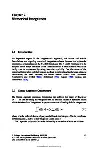
where w(x) is called a weight function. Integration formulas are also referred to as quadrature formulas. The term quadrature coming from the ancient practice of constructing squares with area equivalent to that of a given plane surface. The integrands f (x) or w(x)f (x) in equations (7.31) are assumed to be continuous with known values over the interval a ≤ x ≤ b. The interval [a, b], over which the integral is desired, is divided by (n+1) points into sections with a = x0 < x1 < x2 < . . . < xn = b. This is called partitioning the interval into n-panels. These panels can be of equal lengths or unequal lengths as illustrated in the Þgure 7-1.

Figure 7-1. Partition of interval [a, b] into n-panels.

253 By developing integration formulas for the area under the curve associated with one or more panels, one can repeat the integration formula until the area associated with all panels is calculated. We begin by developing a one-panel formula. Assume that the interval [a, b] is partitioned with equal spacing with a = x0 ,

b = xn ,

h=

b−a , n

xj = x0 + jh,

for j = 0, 1, 2, . . . , n.

(7.32)

The area under the curve y = f (x) between xi−1 and xi is approximated by constructing a straight line interpolating polynomial through the points (xi−1 , yi−1 ) and (xi , yi ) and then integrating this interpolation function. We use yi−1 = f (xi−1 ) and yi = f (xi ) and obtain from the lozenge diagram of Þgure 4-1, with appropriate notation change, the straight line P1 (x) = yi−1 + s∆yi−1 + s(s − 1)

h2 !! f (ξ(x)), 2

where s =

x − xi−1 h

(7.33)

and ∆yi−1 = yi − yi−1 . The area associated with one-panel is then approximated by '

xi

xi−1

f (x) dx ≈

'

xi

P1 (x) dx =

xi−1

'

xi

xi−1

!

$ h2 !! yi−1 + s∆yi−1 + s(s − 1) f (ξ(x)) dx. 2

(7.34)

We use the change of variable for s given by equation (7.33) and integrate the Þrst two terms of equation (7.34) to obtain ! $1 s2 h f (x) dx = h syi−1 + ∆yi−1 = [yi−1 + yi ] 2 2 xi−1 0

'

xi

(7.35)

which is known as the trapezoidal rule since the area of a trapezoid is the average height times the base. Alternatively the trapezoidal rule can be derived by integrating the Lagrange interpolating polynomial P1 (x) =

from xi−1 to xi .

x − xi x − xi−1 f (xi−1 ) + f (xi ) xi−1 − xi xi − xi−1

254 The last integral in equation (7.34) represents an integral of the error term accompanying the approximation polynomial. In order to evaluate this last integral we use the mean value theorem '

xn

f (x)g(x) dx = f (ζ)

xm

'

xn

g(x) dx,

xm < ζ < xn ,

(7.36)

xm

where it is assumed that the functions f, g are continuous in the interval [xm , xn ] and g(x) remains of one sign over the interval. i.e. Either g(x) ≥ 0 or g(x) ≤ 0 over the interval. By integrating the error term of the straight line approximating polynomial one obtains the local error term associated with the trapezoidal rule formula. This integration produces '

xi

h2 !! f (ξ(x)) dx, 2

x − xi−1 , h xi−1 ! 3 $1 ' 1 s2 h3 !! s h3 !! 2 f (ζ) − (s − s) ds = local error = f (ζ) 2 2 3 2 0 0

local error =

local error = −

(s2 − s)

s=

h ds = dx (7.37)

h3 !! f (ζ). 12

The one-panel trapezoidal formula with local error term can be written in either of the forms '

or

xi

h h3 f (x) dx = [yi−1 + yi ] − f !! (ζ) 2 12 xi−1 ' xi h h3 f (x) dx = [f (xi−1 ) + f (xi )] − f !! (ζ) 2 12 xi−1

(7.38)

By partitioning an interval [x0 , xn ] into n + 1 points one can write '

xn

x0

f (x) dx =

n ' ( j=1

xj

f (x) dx.

(7.39)

xj−1

Now one can apply the trapezoidal rule to each of the n-panels. The sum that results gives a representation of the integral over the interval [x0 , xn ]. This representation is called the extended trapezoidal rule or composite trapezoidal rule and can be represented for equal or unequal panel spacing. For unequal panel spacing the extended trapezoidal rule is written '

xn

x0

f (x) dx =

h1 h2 hn (y0 + y1 ) + (y1 + y2 ) + · · · + (yn−1 + yn ) + global error 2 2 2

(7.40)