Received: 21 September 2018 DOI: 10.1002/mma.5387
RESEARCH ARTICLE
Characterisation of multiple conducting permeable objects in metal detection by polarizability tensors P.D. Ledger1
W.R.B. Lionheart2
1 Zienkiewicz Centre for Computational Engineering, College of Engineering, Swansea University Bay Campus, Swansea, Wales 2
School of Mathematics, Alan Turing Building, The University of Manchester, Manchester, England Correspondence P.D. Ledger, Zienkiewicz Centre for Computational Engineering, College of Engineering, Swansea University Bay Campus, Swansea, Wales. Email:
[email protected] Communicated by: W. Sprößig Funding information Engineering and Physical Sciences Research Council, Grant/Award Number: EP/R002134/1 MSC Classification: 35R30; 35B30
A.A.S. Amad1
Realistic applications in metal detection involve multiple inhomogeneousconducting permeable objects, and the aim of this paper is to characterise such objects by polarizability tensors. We show that, for the eddy current model, the leading order terms for the perturbation in the magnetic field, due to the presence of N small conducting permeable homogeneous inclusions, comprises of a sum of N terms with each containing a complex symmetric rank 2 polarizability tensor. Each tensor contains information about the shape and material properties of one of the objects and is independent of its position. The asymptotic expansion we obtain extends a previously known result for a single isolated object and applies in situations where the object sizes are small and the objects are sufficiently well separated. We also obtain a second expansion that describes the perturbed magnetic field for inhomogeneous and closely spaced objects, which again characterises the objects by a complex symmetric rank 2 tensor. The tensor's coefficients can be computed by solving a vector valued transmission problem, and we include numerical examples to illustrate the agreement between the asymptotic formula describing the perturbed fields and the numerical prediction. We also include algorithms for the localisation and identification of multiple inhomogeneous objects. K E Y WO R D S asymptotic expansion, Eddy currents, land mine detection, metal detectors, polarizability tensors
1
I N T RO DU CT ION
There is considerable interest in being able to locate and characterise multiple conducting permeable objects from measurements of mutual inductance between a transmitting and a receiving coil, where the coupling is inductive. An obvious example is in metal detection where the goal is to identify and locate the multiple objects present in a low conducting background. Applications include security screening, archaeological digs, ensuring food safety as well as the search for land mines, and unexploded ordnance and land mines. Other applications include magnetic induction tomography for medical imaging applications and monitoring of corrosion of steel reinforcement in concrete structures. In all these practical applications, the need to locate and distinguish between multiple conducting permeable inclusions is common. This includes benign situations, such as coins and keys accidentally left in a pocket during a security search or a treasure hunter becoming lucky and discovering a hoard of Roman coins, as well as threat situations, where the ...............................................................................................................................................................
This is an open access article under the terms of the Creative Commons Attribution License, which permits use, distribution and reproduction in any medium, provided the original work is properly cited. © 2018 The Authors Mathematical Methods in the Applied Sciences Published by John Wiley & Sons Ltd. Math Meth Appl Sci. 2018;1–31.
wileyonlinelibrary.com/journal/mma
1
2
LEDGER ET AL.
risks need to be clearly identified from the background clutter. For example, in the case of searching for unexploded land mines, the ground can be contaminated by ring-pulls, coins, and other metallic shrapnel, which makes the process of clearing them very slow as each metallic object needs to be dug up with care. Furthermore, conducting objects are also often inhomogeneous and made up of several different metals. For instance, the barrel of a gun is invariably steel while the frame could be a lighter alloy, jacketed bullets have a lead shot and a brass jacket, and modern coins often consist of a cheaper metal encased in nickel or brass alloy. Thus, in practical metal detection applications, it is important to be able to describe both multiple objects and inhomogeneous objects. Magnetic polarizability tensors (MPTs) hold considerable promise for the low-cost characterisation in metal detection. An asymptotic expansion describing the perturbed magnetic field due to the presence of a small conducting permeable object has been obtained by Ammari, Chen, Chen, Garnier, and Volkov,1 which characterises the object in terms of a rank 4 tensor. Ledger and Lionheart have shown that this asymptotic expansion simplifies for orthonormal coordinates and allows a conducting permeable object to be characterised by a complex symmetric rank 2 MPT with an explicit expression for its six coefficients.2 Ledger and Lionheart have also investigated the properties of this tensor,3 and they have written the article4 to explain these developments to the electrical engineering community as well as to show how it applies in several realistic situations. In a previous study,5 they have obtained a complete asymptotic expansion of the magnetic field, which characterises the object in terms of a new class of generalised magnetic polarizability tensors (GMPTs); the rank 2 MPT being the simplest case. The availability of an explicit formula for the MPT's coefficients, and its improved understanding, allows new algorithms for object location and identification to be designed, eg, in an existing study.6 Electrical engineers have applied MPTs to a range of practical metal detection applications, including walk through metal detectors, in line scanners, and demining, eg, previous studies,7-13 see also our article4 for a recent review but without knowledge of the explicit formula described above. Engineers have made a prediction of the form of the response for multiple objects, eg, existing study14 but without an explicit criteria on the size or the distance between the objects in order for the approximation to hold. Grzegorczyk, Barrowes, Shubitidze, Fernández, and O'Neill have applied a time domain approach to classify multiple unexploded ordinance using descriptions related to MPTs.15 Davidson, Abel-Rehim, Hu, Marsh, O'Toole, and Peyton have made measurements of MPTs for inhomogeneous US coins16 and Yin, Li, Withers, and Peyton have also made measurements to characterise inhomogeneous aluminium/carbon-fibre reinforced plastic sheets.17 But, in all cases, without an explicit formula. Our work has the following novelties: Firstly, we characterise rigidly joined collections of different metals (ie, metals touching or held in that configuration by a nonconducting material) by MPTs overcoming a deficiency of our previous work. Secondly, we find that the frequency spectra of the eigenvalues of the real and imaginary parts of the MPT for an inhomogeneous object exhibit multiple nonstationary inflection points and maxima, respectively, and the number of these gives an upper bound on the number of materials making up the object. To achieve this, we revisit the asymptotic formula of Ammari et al1 and our previous work2 and extend it to treat multiple objects by describing the perturbed magnetic field as a sum of terms involving the MPTs associated with each of the inclusions. We also provide a criteria based on the distance between the objects, which determines the situations in which the expression will hold. We derive a second asymptotic expansion that describes the perturbed magnetic field in the case of inhomogeneous objects and, as a corollary, this also describes the magnetic field perturbation in the case of closely spaced objects. In each case, we provide new explicit formulae for the MPTs. We also present algorithms for the localisation and characterisation of objects, which extends those for the isolated object case.1 The paper is organised as follows: In Section 2, the characterisation of a single homogeneous object is briefly reviewed. Section 3 presents our main results for characterising multiple and inhomogeneous objects by MPTs. Sections 4 and 5 contain the details of the proofs for our main results. In Section 6, we present numerical results to demonstrate the accuracy of the asymptotic formulae and presents results of algorithms for the localisation and identification of multiple (inhomogeneous) objects.
2
CHARACTERISAT ION O F A SINGLE CO NDUCTING PERMEABLE OBJECT
We begin by recalling known results for the characterisation of a single homogenous conducting permeable object. Following previous works,1,2 we describe a single inclusion by B𝛼 ∶ = 𝛼B + z, which means that it can be thought of a unit-sized object B located at the origin, scaled by 𝛼 and translated by z. We assume the background is nonconducting and nonpermeable and introduce the position dependent conductivity and permeability as { 𝜎𝛼 =
𝜎∗ in B𝛼 0 in Bc𝛼 ,
{ 𝜇𝛼 =
𝜇∗ in B𝛼 𝜇0 in Bc𝛼 ,
LEDGER ET AL.
3
where 𝜇0 is the permeability of free space and Bc𝛼 ∶= R3 ∖B𝛼 . For metal detection, the relevant mathematical model is the eddy current approximation of Maxwell's equations since 𝜎 ∗ is large and the angular frequency 𝜔 = 2𝜋f is small (see Ammari, Buffa, and Nédélec18 for a detailed justification). Here, the electric and magnetic interaction fields, E𝛼 and H𝛼 , respectively, satisfy the curl equations ∇ × H 𝛼 = 𝜎𝛼 E𝛼 + J 0 ,
∇ × E𝛼 = i𝜔𝜇𝛼 H 𝛼 ,
(1)
in R3 and decay as O(|x|−1 ) for |x| → ∞. In the above equation, J0 is an external current source with support in Bc𝛼 . In absence of an object, the background fields E0 and H0 satisfy (1) with 𝛼 = 0. The task is to find an economical description for the perturbed magnetic field (H𝛼 − H0 )(x) due to the presence of B𝛼 , which characterises the object's shape and material parameters by a small number of parameters separately to its location z. For x away from B𝛼 , the leading order term in an asymptotic expansion for (H𝛼 − H0 )(x) as 𝛼 → 0 has been derived by Ammari et al.1 We have shown that this reduces to the simpler form2,4 * (H 𝛼 − H 0 )(x)i = (D2x G(x, z))i𝑗 ([𝛼B])𝑗k (H 0 (z))k + (R(x))i 1 = (3̂r ⊗ r̂ − I)i𝑗 ([𝛼B])𝑗k (H 0 (z))k + (R(x))i . 4𝜋r 3
(2)
In the above, G(x, z) ∶ = 1∕(4𝜋|x − z|) is the free space Laplace Green's function, r ∶= x − z, r = |r| and r̂ = r∕r and I is the rank 2 identity tensor. The term R(x) quantifies the remainder, and it is known that |R| ⩽ C𝛼 4 ||H 0 ||W 2,∞ (B𝛼 ) . The result holds when 𝜈 ∶ = 𝜎 ∗ 𝜇 0 𝜔𝛼 2 = O(1) (this includes the case of fixed 𝜎 ∗ , 𝜇∗ , 𝜔 as 𝛼 → 0) and requires that the background field be analytic in the object. Note that (2) involves the evaluation of the background field within the object (usually at it's centre), ie, H0 (z). The complex symmetric rank 2 tensor [𝛼B] ∶= −[𝛼B] + [𝛼B] in this asymptotic expansion, which depends on 𝜔, 𝜎 ∗ , 𝜇 ∗ ∕𝜇0 , 𝛼 and the shape of B, but is independent of z, is the MPT, and its coefficients can be computed from i𝜈𝛼 3 e𝑗 · 𝝃 × (𝜽k + ek × 𝝃)d𝝃, ∫B 4 ( ) ( ) 𝜇0 1 3 e𝑗 · ek + e𝑗 · ∇𝜉 × 𝜽k d𝝃. ( [𝛼B])𝑗k ∶= 𝛼 1 − 𝜇∗ ∫B 2
(3a)
([𝛼B])𝑗k ∶= −
(3b)
These, in turn, rely on the vectoral solutions 𝜽k , k = 1, 2, 3, to the transmission problem ∇𝜉 × 𝜇∗−1 ∇𝜉 × 𝜽k − i𝜔𝜎∗ 𝛼 2 𝜽k = i𝜔𝜎∗ 𝛼 2 ek × 𝝃 ∇𝜉 · 𝜽k = 0, [n × 𝜽k ]Γ = 𝟎,
∇𝜉 ×
𝜇0−1 ∇𝜉
× 𝜽k = 𝟎
in B,
[n × 𝜇−1 ∇𝜉 × 𝜽k ]Γ = −2[𝜇−1 ]Γ n × ek 𝜽k = O(|𝝃| ) −1
(4a) 3
̄ in B ∶= R ∖B,
(4b)
on Γ ∶= 𝜕B,
(4c)
as |𝝃| → ∞,
(4d)
c
where [·]Γ denotes the jump of the function over Γ and 𝝃 is measured from an origin chosen to be in B. In an existing study,3 we have presented numerical results for the frequency behaviour of the coefficients of for a variety of simply and multiply connected objects. These have been obtained by applying an hp-finite element method to solve (4) for 𝜽k , k = 1, 2, 3 and then to compute using (3). Our previously presented results have exhibited excellent agreement with for MPTs previously presented in the electrical engineering literature. Pratical applications of the asymptotic formula have been discussed in another study.4
3
MAIN RESULTS
The asymptotic formula given in (2) is for a single isolated homogenous object. But, as described in the introduction, for realistic metal detection scenarios, measurements of the perturbed magnetic field often relate to field changes caused by the presence of multiple objects or inhomogeneous objects. The purpose of this work is to extend the description to the * In order to simplify notation, we drop the double check on and the single check on , which was used in2 to denote two and one reduction(s) in rank, respectively. We recall that = ()𝑗k e𝑗 ⊗ ek by the Einstein summation convention where we use the notation ej to denote the jth unit vector. We will denote the jth component of a vector u by u · ej = (u)j and the j, kth coefficient of a rank 2 tensor by 𝑗k .
4
LEDGER ET AL.
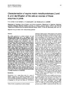
FIGURE 1 Illustration of a typical situation of N = 3 objects with B𝜶 = ∪Nn=1 (B𝛼 )(n) = 𝛼 (n) B(n) + z(n) such that they are not closely spaced
where each object (B𝛼 )(n) is a sphere, 𝛼 (n) is the radius of the nth sphere, z(n) describes the translation of the nth sphere from the origin, and B = B(1) = B(2) = B(3) is a unit sphere positioned at the origin
cases of well separated multiple homogeneous objects and inhomogeneous objects. As a result of corollary, our second main result also describes the case of objects that of objects that are closely spaced. Below, we summarise the main results of our paper.
3.1
Multiple homogeneous objects that are sufficiently well spaced
We consider N homogenous-conducting permeable objects of the form (B𝛼 )(n) = 𝛼 (n) B(n) + z(n) † with Lipschitz boundaries where, for the nth object, B(n) denotes a corresponding unit sized object located at the origin, 𝛼 (n) denotes the object's size, and z(n) the object's translation from the origin. The union of all objects is B𝜶 ∶= ∪Nn=1 (B𝛼 )(n) where we use a bold subscript 𝜶 to denote the possibility that each object in the collection can have a different size. We also employ the same notation for the fields E𝜶 and H𝜶 , which satisfy (1). An illustration of a typical configuration is shown in Figure 1. In this figure, there are N = 3 objects, which are the spheres (B𝛼 )(n) = 𝛼 (n) B(n) + z(n) , n = 1, 2, 3, where, for the nth object, 𝛼 (n) is its size (here its radius), and z(n) is its translation from the origin. In the presented case, B = B(1) = B(2) = B(3) is a unit sphere located at the origin although, in practice, the objects do not need to have the same shape. We generalise the definitions of 𝜇𝛼 and 𝜎 𝛼 previously stated in Section 2 to { (n) { (n) 𝜎∗ in (B𝛼 )(n) 𝜇∗ in (B𝛼 )(n) 𝜎𝜶 = , 𝜇 = , 𝜶 0 in Bc𝜶 𝜇0 in Bc𝜶 where Bc𝜶 ∶= R3 ∖B𝜶 and set 𝜎min ⩽ 𝜎∗(n) ⩽ 𝜎max and 𝜇min ⩽ 𝜇∗(n) ⩽ 𝜇max for n = 1, … , N. We introduce 𝜈min ⩽ 𝜈 (n) ∶= 𝜔𝜇0 𝜎∗(n) (𝛼 (n) )2 ⩽ 𝜈max and set 𝛼min = min 𝛼 (n) , 𝛼max = max 𝛼 (n) and require that the parameters of the inclusions be n=1, … ,N
n=1, … ,N
such that 𝜈max = O(1), which implies that 𝜈 = O(1). The task is then to provide a low-cost description of (H𝜶 − H0 )(x) for x away from B𝜶 . This is accomplished through the following result. (n)
Theorem 3.1. For the arrangement B𝜶 of N homogeneous conducting permeable objects (B𝛼 )(n) = 𝛼 (n) B(n) + z(n) with |𝜕(B𝛼 )(n) −𝜕(B𝛼 )(m) | ⩾ 𝛼max and parameters such that 𝜈 (n) = O(1) , the perturbed magnetic field at positions min
n,m=1, … ,N,n≠m
x away from B𝜶 satisfies N ∑ (H𝜶 − H0 )(x)i = (D2x G(x, z(n) ))i𝑗 ([𝛼 (n) B(n) ])𝑗k (H0 (z(n) ))k + (R(x))i , n=1
where 4 |R(x)| ⩽ C𝛼max ||H0 ||W 2,∞ (B ) , 𝜶
†
Note no summation over n is implied.
(5)
LEDGER ET AL.
5
uniformly in x in any compact set away from B𝜶 . The coefficients of the complex symmetric MPTs [𝛼 (n) B(n) ] = −[𝛼 (n) B(n) ] + [𝛼 (n) B(n) ], n = 1, … , N, can be computed independently for each of the objects 𝛼 (n) B(n) using the expressions i𝜈 (n) (𝛼 (n) )3 𝝃 (n) × (𝜽(n) + ek × 𝝃 (n) )d𝝃 (n) , (6a) ([𝛼 (n) B(n) ])𝑗k ∶= − e𝑗 · k ∫B(n) 4 ( ) ( ) 𝜇0 1 (n) (n) (n) 3 e𝑗 · ek + e𝑗 · ∇𝜉 × 𝜽(n) d𝝃 (n) . ( [𝛼 B ])𝑗k ∶= (𝛼 ) 1 − (n) (6b) k ∫B(n) 2 𝜇∗ These, in turn, rely on the vectoral solutions 𝜽(n) , k = 1, 2, 3, to the transmission problem k ∇𝜉 × (𝜇∗(n) )−1 ∇𝜉 × 𝜽(n) − i𝜔𝜎∗(n) (𝛼 (n) )2 𝜽(n) = i𝜔𝜎∗(n) (𝛼 (n) )2 ek × 𝝃 (n) k k ∇𝜉 · 𝜽(n) = 0, k
∇𝜉 × 𝜇0−1 ∇𝜉 × 𝜽(n) =𝟎 k [n ×
𝜽(n) ] (n) k Γ
(7a)
in (B(n) )c ,
(7b)
on Γ ,
(7c)
on Γ(n) ,
(7d)
as |𝝃 | → ∞,
(7e)
=𝟎
(n)
[n × 𝜇−1 ∇𝜉 × 𝜽(n) ] (n) = −2[𝜇−1 ]Γ(n) n × ek k Γ 𝜽(n) k
in B(n) ,
= O(|𝝃 | ) (n) −1
(n)
where (B(n) )c ∶= R3 ∖B(n) , Γ(n) ∶ = 𝜕B(n) and 𝝃 (n) is measured from an origin chosen to be in B(n) . Proof. The result follows from by using a tensor representation of the asymptotic formula in Theorem 4.8, which is an extension of Theorem 3.2 obtained in a previous work1 for N sufficiently well-spaced objects. A tensor representation of this result leads to each of the N objects being characterised by a rank 4 tensor. Then, by considering each object in turn and repeating the same arguments as in Theorem 3.1 in another study,2 which exploits the skew symmetries of the tensor coefficients, the result stated in (5) is obtained. The symmetry of [𝛼 (n) B(n) ] follows from repeating the arguments in Lemma 4.4 in the previous study.2 Corollary 3.2. For the case of N = 1 then B𝜶 becomes B𝛼 , H𝜶 becomes H𝛼 , and Theorem 3.1 reduces to the case of a single homogenous object as obtained in previous works1,2 and described in Section 2.
3.2
Single inhomogeneous object
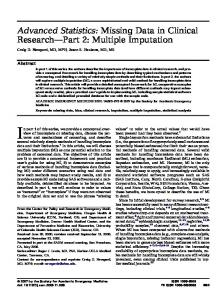
⋃N ⋃N (n) + z = 𝛼B + z describes a single object comprised of N constitute parts, B(n) , In this case, B𝛼 ∶= n=1 B(n) 𝛼 = 𝛼 𝛼 n=1 B such that there is a single common size parameter 𝛼, the configuration B contains the origin, and z is a single translation, (n) as 𝛼 is the same for all as illustrated in Figure 2. Notice that for the inhomogeneous case, we use B(n) 𝛼 rather than (B𝛼 ) n, and we revert to the use of nonbold 𝛼 subscripts for the fields E𝛼 and H𝛼 , which satisfy (1).
FIGURE 2 Illustration of a typical situation of an inhomogeneous object consisting of N = 3 subdomains such that the complete object is N (n) B𝛼 = ∪Nn=1 B(n) + z = 𝛼B + z 𝛼 = 𝛼 ∪n=1 B
6
LEDGER ET AL.
The material parameters of the constitute parts of the object B𝛼 are { (n) { (n) 𝜎∗ in B(n) 𝜇∗ in B(n) 𝛼 𝛼 𝜎𝛼 = , 𝜇 = , 𝛼 c 0 in B𝛼 𝜇0 in Bc𝛼 where Bc𝛼 ∶= R3 ∖B𝛼 , and we drop the subscript 𝛼 on 𝜇 and 𝜎 when considering the object B. We redefine 𝜈min ⩽ 𝜈 (n) ∶= 𝜔𝜇𝜎∗(n) 𝛼 2 ⩽ 𝜈max with the same requirements on 𝜈max as before. The task is then to provide a low-cost description of (H𝛼 − H0 )(x) for x away from B𝛼 . This is accomplished through the following result. Theorem 3.3. For an inhomogeneous object, B𝛼 = 𝛼B + z made up of N constitute parts with parameters such that 𝜈min ⩽ 𝜈 (n) ⩽ 𝜈max the perturbed magnetic field at positions x away from B𝛼 satisfies (H𝛼 − H0 )(x)i = (D2x G(x, z))i𝑗 ( [𝛼B])𝑗k (H0 (z))k + (R(x))i ,
(8)
where |R(x)| ⩽ C𝛼 4 ||H0 ||W 2,∞ (B𝛼 ) , uniformly in x in any compact set away from B𝛼 . The coefficients of the complex symmetric MPT [𝛼B] = − [𝛼B] + [𝛼B] are given by N i𝛼 3 ∑ (n) 𝜈 e𝑗 · 𝝃 × (𝜽k + ek × 𝝃)d𝝃, (9a) ( [𝛼B])𝑗k ∶= − ∫B(n) 4 n=1 ( ) N ( ) ∑ ( ) 𝜇 1 0 [𝛼B] 𝑗k ∶= 𝛼 3 e𝑗 · ek + e𝑗 · ∇𝜉 × 𝜽k d𝝃, (9b) 1 − (n) ∫B(n) 2 𝜇∗ n=1 which, in turn, rely on the vectoral solutions 𝜽k , k = 1, 2, 3, to the transmission problem ∇𝜉 × 𝜇−1 ∇𝜉 × 𝜽k − i𝜔𝜎𝛼 2 𝜽k = i𝜔𝜎𝛼 2 ek × 𝝃 ∇𝜉 · 𝜽k = 0, [n × 𝜽k ]Γ = 𝟎,
∇𝜉 × 𝜇0−1 ∇𝜉 × 𝜽k = 𝟎 [n × 𝜇−1 ∇𝜉 × 𝜽k ]Γ = −2[𝜇−1 ]Γ n × ek 𝜽k = O(|𝝃|−1 )
in B,
(10a)
in Bc ∶= R3 ∖B, on Γ, as |𝝃| → ∞,
(10b) (10c) (10d)
where 𝝃 is measured from the centre of B and, in this case, Γ ∶= 𝜕B ∪ {𝜕B(n) ∩ 𝜕B(n) , n, m = 1, … , N, n ≠ m}. Proof. The result follows from by using a tensor representation of the asymptotic formula in Theorem 5.3, which is an extension of Theorem 3.2 obtained in the previous research1 for an homogeneous object to the inhomogeneous case. Using a tensor representation of this result leads to the object being characterised in terms of a rank 4 tensor. Then, by repeating the same arguments as in Theorem 3.1 in another study,2 which exploits the skew symmetries of the tensor coefficients, the result stated in (8) is obtained. The symmetry of [𝛼B] follows from repeating the arguments in Lemma 4.4 in the previous study.2 Corollary 3.4. For the case of N = 1 then B𝛼 becomes B𝛼 and Theorem 3.3 reduces to the case of a single homogenous object as obtained in existing works1,2 and described in Section 2. Corollary 3.5. Theorem 3.3 also immediately applies to objects that are closely spaced and, in this case, B𝛼 = 𝛼B + z implies a single size parameter 𝛼 and a single translation z for the configuration B. An illustration of a typical configuration is shown in Figure 3. In this figure, there are N = 3 objects consisting of three spheres configured such that they scale and translate together according to 𝛼 and z, respectively, and, in this case, B is the combined configuration of three (larger) spheres with different radii and with centres located away from the origin. Remark 3.6. The applicability of Theorem 3.3 to closely spaced objects is expected to be limited since, in order to compute the characterisation, prior knowledge of the multiple object configuration (ie, location and orientation with respect to each other) is required, which, in practice, will not be the case. The formula also requires that the objects be closely spaced as there is a single scaling parameter and single translation that describes the configuration, but prior knowledge of the location of the configuration is not required. Instead, this result is expected to be of more practical value in the description of inhomogeneous objects where the configuration of the different regions of an object will be known in advance.
LEDGER ET AL.
7
⋃N (n) B(n) + z = 𝛼B + z where 𝛼 =𝛼 n=1 B each object is a sphere, 𝛼 is a single scaling parameter, z describes their translation of the configuration from the origin
FIGURE 3 Illustration of a typical situation of N = 3 closely spaced objects of the form B𝛼 =
⋃N
n=1
Remark 3.7. The translation invariance of the MPT coefficients described by Ammari et al's Proposition 5.2 6 and the tensor transformation rules described in the proof of Theorem 3.1 in the previous study 2 carry over immediately to the rank 2 MPTs defined in (6) and (9).
4 4.1
R E S U LT S FO R T HE PROOF O F THEO REM 3.1 Elimination of the current source
Recall from the previous research1 that {
} u
X 𝜶 (R ) ∶ =
u∶ √ ∈ L (R ) , ∇ × u ∈ L (R ) , ∇ · u = 0 in 1 + |x|2 { } u · n|+ dx = 0 , X̃ 𝜶 (R3 ) ∶ = u ∶ u ∈ X 𝜶 (R3 ), ∫Γ 3
2
3 3
2
3 3
Bc𝜶
,
𝜶
and the weak solution for the interaction field is: Find E𝜶 ∈ X̃ 𝜶 such that a𝛼 (E𝜶 , v) = (J 0 , v)R3 = (J 0 , v)supp (J 0 )
∀v ∈ X̃ 𝜶 ,
where (·, ·)Ω denotes the standard L2 inner product over Ω. In a departure from the previous study,1 we have, for multiple objects, that a(u, v) ∶= (𝜇0−1 ∇ × u, ∇ × v)Bc + (𝜇𝜶−1 ∇ × u, ∇ × v)B − i𝜔(𝜎𝜶 u, v)B . 𝜶
𝜶
𝜶
Noting that the weak solution for the background field is: Find E0 ∈ X̃ 𝜶 such that (𝜇0−1 ∇ × E0 , ∇ × v)R3 = (J 0 , v)supp (J 0 )
∀v ∈ X̃ 𝜶 ,
we can write: Find E𝜶 ∈ X̃ 𝜶 such that a(E𝜶 , v) = (𝜇0−1 ∇ × E0 , ∇ × v)R3
∀v ∈ X̃ 𝜶 ,
which eliminates the current source. We also obtain that (𝜇0−1 ∇ × (E𝜶 − E0 ), ∇ × v)Bc + (𝜇𝜶−1 ∇ × (E𝜶 − E0 ), ∇ × v)B
𝜶
𝜶
− i𝜔(𝜎𝜶 (E𝜶 − E0 ), v)B = ((𝜇𝜶−1 − 𝜇0 )∇ × E0 , ∇ × v)B 𝜶
+ i𝜔(𝜎𝜶 E0 , v)B . 𝜶
𝜶
(11)
8
LEDGER ET AL.
4.2
Energy estimates
In the existing work,1 a vector field F(x) was introduced such that its curl is equal to the first two terms of Taylor's series expansion of ∇ × E0 about z for |x − z| → 0 for the case of a single object B𝛼 . This was possible as the current source J0 is 1 ∇ × E0 (x) is analytic where the expansion is applied. We extend this supported away from the object and so H 0 (x) = i𝜔𝜇 0 to the multiple object case by requiring that J0 be supported away from B𝜶 and introduce the following for n = 1, … , N 1 1 (∇z × E0 (z))(z(n) ) × (x − z(n) ) + Dz (∇z × E0 (z))(z(n) )(x − z(n) ) × (x − z(n) ), 2 3 ∇ × F (n) (x) = (∇z × E0 (z))(z(n) ) + Dz (∇z × E0 (z))(z(n) )(x − z(n) ), F (n) (x) =
so that
i𝜔𝜇0 i𝜔𝜇0 H 0 (z(n) ) × (x − z(n) ) + Dz (H 0 (z))(z(n) )(x − z(n) ) × (x − z(n) ), 2 3 ) ( ∇ × F (n) (x) = i𝜔𝜇0 H 0 (z(n) ) + Dz (H 0 (z))(z(n) )(x − z(n) ) . F (n) (x) =
In other words, ∇ × F(n) (x) is the first two terms in a Taylor series of i𝜔𝜇0 H0 (x) about z(n) as |x − z(n) | → 0 and so ||i𝜔𝜇0 H 0 (x) − ∇ × F (n) ||L∞ ((B𝛼 )(n) ) ⩽ C(𝛼 (n) )2 ||∇ × E0 ||W 2,∞ ((B𝛼 )(n) ) , 3
||i𝜔𝜇0 H 0 (x) − ∇ × F (n) ||L2 ((B𝛼 )(n) ) ⩽ C(𝛼 (n) ) 2 ||i𝜔𝜇0 H 0 (x) − ∇ × F (n) ||L∞ ((B𝛼 )(n) ) 7
⩽ C(𝛼 (n) ) 2 ||∇ × E0 ||W 2,∞ ((B𝛼 )(n) ) ,
(12)
where here and in the following C denotes a generic constant unless otherwise indicated. Remark 4.1. Higher order Taylor series could be considered (as previously in another study5 for the case of a single object) and lead to a more accurate representation of the field in terms of GMPTs. However, in order for such a representation to apply, there will be further implications in the allowable distance between the objects. The introduction of F(n) (x) motivates the introduction of the following problem: Find w(n) ∈ X̃ 𝜶 such that (𝜇0−1 ∇ × w(n) , ∇ × v)((B𝛼 )(n) )c + ((𝜇∗(n) )−1 ∇ × w(n) , ∇ × v)(B𝛼 )(n) − i𝜔(𝜎∗(n) w(n) , v)(B𝛼 )(n) = ((𝜇0−1 − (𝜇∗(n) )−1 )∇ × F (n) , ∇ × v)(B𝛼 )(n) + i𝜔(𝜎∗(n) F (n) , v)(B𝛼 )(n)
∀v ∈ X̃ 𝜶 ,
(13)
where ((B𝛼 )(n) )c ∶= R3 ∖(B𝛼 )(n) . By the addition of such problems, we have ( −1 𝜇0 ∇ × w, ∇ × v)Bc + (𝜇𝜶−1 ∇ × w𝜶 , ∇ × v)B − i𝜔(𝜎𝜶 w𝜶 , v)B 𝜶
𝜶
∑
𝜶
N
+
(𝜇0−1 ∇ × w(m) (1 − 𝛿mn ), ∇ × v)(B𝛼 )(n) = ((𝜇0−1 − (𝜇𝜶−1 ))∇ × F 𝜶 , ∇ × v)B
𝜶
n,m=1
+ i𝜔(𝜎𝜶 F 𝜶 , v)B , 𝜶
where w ∶=
∑N n=1
w(n) , w𝜶 = w(n) in (B𝛼 )(n) and F 𝜶 = F (n) in (B𝛼 )(n) .
(14)
LEDGER ET AL.
9
We also remark that associated with (13) is the strong form ∇ × (𝜇∗(n) )−1 ∇ × w(n) − i𝜔𝜎∗(n) w(n) = i𝜔𝜎∗(n) F (n)
in (B𝛼 )(n) ,
(15a)
∇ × 𝜇0−1 ∇ × w(n) = 𝟎
in ((B𝛼 )(n) )c ,
(15b)
∇ · w(n) = 0 ] [ n × w(n) (Γ )(n) = 𝟎
in ((B𝛼 )(n) )c ,
(15c)
on (Γ𝛼 )(n) ∶= 𝜕(B𝛼 )(n) ,
(15d)
on (Γ𝛼 )(n) ,
(15e)
as |x| → ∞,
(15f)
𝛼
] [ n × 𝜇−1 ∇ × w(n) (Γ
𝛼)
(n)
= −(𝜇0−1 − (𝜇∗(n) )−1 )n × ∇ × F (n)
w(n) = O(|x|−1 ) which follows from using (𝜇0−1 − (𝜇∗(n) )−1 )(∇ × F (n) , ∇ × v)(B𝛼 )(n) = (𝜇0−1 − (𝜇∗(n) )−1 ) =
[ ∫(Γ𝛼 )(n)
∫(Γ𝛼 )(n)
∇ × F (n) × n · vdx
] 𝜇−1 ∇ × F (n) × n (Γ
𝛼)
(n)
· vdx.
Lemma 4.2. For objects (B𝛼 )(n) and (B𝛼 )(m) with n ≠ m, we have that 7
𝛼2 ||∇ × w ||L2 ((B𝛼 )(m) ) ⩽ C (m) max (n) 2 ||∇ × E0 ||W 2,∞ ((B𝛼 )(n) ∪(B𝛼 )(m) ) . |z − z | (n)
(n)
, which, without loss of generality, we assume the origin to be in B(n) . We set w(n) (x) = Proof. Introducing 𝝃 (n) = x−z 𝛼 (n) ( (n) ) ( ) (n) (n) (n) x−z(n) x−z (n) (n) (n) (n) (n) = 𝛼 . Note that w(n) 𝛼 (n) w(n) w (𝝃 ) and so ∇ × w (x) = ∇ × w (𝝃 ) = ∇ × w x 𝜉 𝜉 0 0 0 0 0 (𝝃 ) satisfies 𝛼 (n) 𝛼 (n) (n) (n) 2 (n) (n) (n) 2 ∇𝜉 × (𝜇∗(n) )−1 ∇𝜉 × w(n) 0 − i𝜔𝜎∗ (𝛼 ) w0 = i𝜔𝜎∗ (𝛼 )
[(𝛼 (n) )−1 F (n) (z(n) + 𝛼 (n) 𝝃 (n) )] ∇𝜉 × 𝜇0−1 ∇𝜉 × w(n) 0 =𝟎 ∇𝜉 · w(n) 0 =0 [ ] n × w(n) =𝟎 0 (n) [ ]Γ n × 𝜇−1 ∇𝜉 × w(n) = − (𝜇0−1 − (𝜇∗(n) )−1 ) 0
in B(n) , in (B(n) )c ,
(16b)
in (B(n) )c ,
(16c)
on Γ(n) ,
(16d)
Γ(n)
n × ∇𝜉 × F (n) (z(n) + 𝛼 (n) 𝝃 (n) ) (n) −1 w(n) 0 = O(|𝝃 | )
(16a)
on Γ(n) , as |𝝃 (n) | → ∞.
(16e) (16f)
(n) −1 (n) From the above, we have that |w(n) 0 | ⩽ C|𝝃 | ||∇ × E 0 ||W 2,∞ ((B𝛼 )(n) ) for sufficiently large |𝝃 | and so we estimate (n) −2 that |∇𝜉 × w(n) 0 | ⩽ C|𝝃 | ||∇ × E0 ||W 2,∞ ((B𝛼 )(n) ) for the same case. Thus, for m ≠ n, ( )1∕2 2 | (m) (n) (m) 3 (n) (m) (m) (m) | = (𝛼 ) ||∇ × w ||L2 (B(m) |∇ × w (𝛼 𝝃 + z )| d𝝃 𝛼 ) | ∫B(m) | x ( )1∕2 ( (m) (m) )2 | 𝛼 𝝃 + z(m) − z(n) || (m) | (n) (m) 3 = (𝛼 ) |∇ × w0 | d𝝃 | ∫B(m) | 𝜉 𝛼 (n) | | −2 (m) (n) 3 |z − z || ⩽ C(𝛼 (m) ) 2 || | ||∇ × E0 ||W 2,∞ ((B𝛼 )(n) ) (n) 𝛼 | | 7
⩽C
2 𝛼max
||∇ × E0 ||W 2,∞ ((B𝛼 )(n) ∪(B𝛼 )(m) ) , |z(m) − z(n) |2 | | where we have used ||∇ × E0 ||W 2,∞ ((B𝛼 )(n) ) ⩽ ||∇ × E0 ||W 2,∞ ((B𝛼 )(n) ∪(B𝛼 )(m) ) .
10
LEDGER ET AL.
FIGURE 4 Illustration to show how each B(n) can be configured differently provided that the origin lies within the object. Consequently d(1),(2) = |z(1) − z(2) | will be minimum when the objects B(1) and B(2) are configured such that the origin is a suitable point on the boundaries of these objects
Corollary 4.3. Given the description (B𝛼 )(n) = 𝛼 (n) B(n) + z(n) , we are free to configure B(n) in different ways provided that the origin lies at a point in B(n) (similarly with (B𝛼 )(m) = 𝛼 (m) B(m) + z(m) ) . Thus, |z(m) − z(n) | will be smallest when the min |𝜕(B𝛼 )(n) − origin lies in the boundaries of the objects, as illustrated in Figure 4. Requiring that |z(m) − z(n) | = n,m=1, … ,N,n≠m
𝜕(B𝛼 )(m) | > C > 𝛼max then Lemma 4.2 implies that 7
2 ||∇ × w(n) ||L2 (B(m) ⩽ C𝛼max ||∇ × E0 ||W 2,∞ ((B𝛼 )(n) ∪(B𝛼 )(m) ) . 𝛼 )
The following Lemma extends Ammari et al's Lemma 3.2 1 to the case of N multiple objects, when they are sufficiently well spaced. Lemma 4.4. Provided that
min
n,m=1, … ,N,n≠m
|𝜕(B𝛼 )(n) − 𝜕(B𝛼 )(m) | ≥ 𝛼max , there exists a constant C such that 7
−1 2 ||∇ × (E𝜶 − E0 − w(n) )||L2 ((B𝛼 )(n) ) ⩽ C(𝜈max + |1 − 𝜇r,max |)𝛼max ||∇ × E0 ||W 2,∞ (B ) , 𝜶
9 2
−1 ||(E𝜶 − E0 − (w(n) + Φ(n) ))||L2 ((B𝛼 )(n) ) ⩽ C(𝜈max + |1 − 𝜇r,max |)𝛼max ||∇ × E0 ||W 2,∞ (B ) , 𝜶
for n = 1, … , N where 𝜇r,max ∶=
maxn = 1, … ,N 𝜇(n) ∕𝜇0 . * {
Proof. We start by proceeding along the lines presented in1 and introduce Φ(n) = (n) −Δ𝜙(n) 0 = −∇ · F
(n) ∇𝜙(n) 0 in (B𝛼 ) where (n) ∇𝜙̃ 0 in ((B𝛼 )(n) )c
in (B𝛼 )(n) ,
(n) (n) −𝜕n 𝜙(n) 0 = (E0 (x) − F (x)) · n on (Γ𝛼 ) ,
∫(B𝛼 )(n)
𝜙𝛼(n) dx = 0,
1 ̃ with 𝜙̃ (n) 0 being the solution of an exterior problem in an analogous way to 𝜙0 in the previous study. Using (11) and (14) (and after multiplying by 𝜇0 ), we can deduce that
A ∶ = (∇ × (E𝜶 − E0 − (w + Φ)), ∇ × v)Bc
𝜶
+ (𝜇0 𝜇𝜶−1 ∇ × (E𝜶 − E0 − (w𝜶 + Φ𝜶 )), ∇ × v)B
𝜶
− i𝜔𝜇0 (𝜎𝜶 (E𝜶 − E0 − (w𝜶 + Φ𝜶 )), v)B
𝜶
= 𝜇0 ((𝜇0−1 − 𝜇𝜶−1 )∇ × (E0 − F 𝜶 ), ∇ × v)B
(17)
𝜶
+ i𝜔𝜇0 (𝜎𝜶 (E0 + Φ𝜶 − F 𝜶 ), v)B
𝜶
+
N ∑ n,m=1
(∇ × (w(m) + Φ(m) ), ∇ × v)(B𝛼 )(n) (1 − 𝛿mn )
∀v ∈ X̃ 𝛼 ,
LEDGER ET AL.
where Φ =
11
∑N n=1
Φ(n) and Φ𝜶 = Φ(n) in (B𝛼 )(n) . Choosing v = E𝜶 − E0 − (w𝜶 + Φ𝜶 ) then we have that ||∇ × (E𝜶 − E0 − (w(n) + Φ(n) ))||2 2
L (B(n) 𝛼 )
⩽ ||∇ × (E𝜶 − E0 − (w𝜶 + Φ𝜶 ))||2L2 (B ) 𝜶
⩽ |A|. Also, by application of the Cauchy-Schwartz inequality, we can check that |A| ⩽ A1 + A2 + A3 , where
(18)
) | | ( A1 ∶ = |𝜇0 (𝜇0−1 − 𝜇𝜶−1 )(∇ × (E0 − F 𝜶 )), ∇ × v B | | | ⩽ C max |1 − (𝜇r(n) )−1 |||∇ × (E0 − F 𝜶 )||L2 (B ) ||∇ × v||L2 (B ) 𝜶
n=1, … ,N
𝜶
(N ∑ −1 ⩽ C|1 − 𝜇r,max | ||∇ × (E0 − F (n) )||2 2
𝜶
)1∕2
L (B(n) 𝛼 )
n=1
(19)
||∇ × v||L2 (B ) 𝜶
7
−1 2 ⩽ C|1 − 𝜇r,max |𝛼max ||∇ × E0 ||W 2,∞ (B ) ||∇ × v||L2 (B ) , 𝜶
𝜶
A2 ∶ = ||𝜔𝜇0 (𝜎𝜶 (E0 + Φ𝜶 − F 𝜶 ), v)B || (N )1∕2 ∑( )2 (n) (n) ⩽ C𝜔𝜇0 𝜎max 𝛼max ||∇ × v||L2 (B ) (𝛼 )||∇ × (E0 − F )||L2 ((B𝛼 )(n) ) 𝜶
𝜶
n=1
(N )1∕2 ∑( )2 ⩽ C𝜈max 𝛼max ||∇ × v||L2 (B ) ||∇ × E0 ||W 2,∞ ((B𝛼 )(n) )
(20)
7 2
𝜶
n=1 7
2 ⩽ C𝜈max 𝛼max ||∇ × E0 ||W 2,∞ (B ) ||∇ × v||L2 (B ) , 𝜶
𝜶
|∑ | | N | (m) (m) | A3 ∶ = | (∇ × (w + Φ ), ∇ × v)B(m) (1 − 𝛿mn )|| 𝛼 |n,m=1 | | | ( N ) ∑ ⩽C (1 − 𝛿mn )||∇ × w(m) ||L2 ((B𝛼 )(n) ) ||∇ × v||L2 (B ) .
(21)
𝜶
n,m=1
To bound A1 and A2 we have used (12), 9
||E0 + Φ(n) − F (n) ||L2 ((B𝛼 )(n) ) ⩽ C𝛼 (n) ||∇ × (E0 − F (n) )||L2 ((B𝛼 )(n) ) ⩽ C(𝛼 (n) ) 2 ||∇ × E0 ||W 2,∞ ((B𝛼 )(n) ) ,
(22)
and applied similar arguments to the previous study.1 The terms A3 does not appear in the single object case and min |𝜕B(n) − 𝜕B(m) | > dictates the minimum spacing for which the bound holds. Requiring that |z(m) − z(n) | = n,m=1, … ,N,n≠m
C > 𝛼max and applying Corollary 4.3 then 7
2 A3 ⩽ C𝛼max ||∇ × E0 ||W 2,∞ (B ) ||∇ × v||L2 (B ) . 𝜶
(23)
𝜶
Using (19), (20), and (23) in (18) we find that ⩽ ||∇ × (E𝜶 − E0 − (w𝜶 + Φ𝜶 ))||L2 (B ) ||∇ × (E𝜶 − E0 − (w(n) + Φ(n) ))||L2 (B(n) 𝛼 ) ( ) 72 −1 ⩽ C 𝜈max + |1 − 𝜇r,max | 𝛼max ||∇ × E0 ||W 2,∞ (B ) , 𝜶
𝜶
⩽ 𝛼 ||∇ × (E𝜶 − E0 − (w and by additionally using ||E𝜶 − E0 − (w + Φ )||L2 (B(n) 𝛼 ) (n) (n) , this completes the proof. E0 − (w + Φ ))||L2 (B(n) 𝛼 ) (n)
(n)
(n)
(n)
+ Φ ))||L2 (B(n) ⩽ 𝛼max ||∇ × (E𝜶 − 𝛼 ) (n)
1 By recalling the definition of w(n) 0 (𝝃) stated in Lemma 4.2, Ammari's et al's Theorem 3.1 in the case of multiple sufficiently well spaced objects becomes
12
LEDGER ET AL.
Theorem 4.5. Provided that
min
n,m=1, … ,N,n≠m
|𝜕(B𝛼 )(n) − 𝜕(B𝛼 )(m) | ⩾ 𝛼max , there exists a constant C such that
( ( ))‖ ‖ x − z(n) ‖ ‖ (n) −1 |) ⩽ C(𝜈max + |1 − 𝜇r,max ‖∇ × E𝜶 − E0 − 𝛼 (n) w0 ‖ (n) ‖ ‖2 𝛼 ‖ ‖L ((B𝛼 )(n) ) 7
2 ||∇ × E0 ||W 2,∞ (B ) , 𝛼max 𝜶
( ( ) )‖ ‖ x − z(n) ‖ (n) (n) ‖ −1 |) ⩽ C(𝜈max + |1 − 𝜇r,max + Φ ‖ ‖E𝜶 − E0 − 𝛼 (n) w0 (n) ‖2 ‖ 𝛼 ‖L ((B𝛼 )(n) ) ‖ 9
2 ||∇ × E0 ||W 2,∞ (B ) . 𝛼max 𝜶
Proof. The result immediately follows from Lemma 4.4 and the definition of w(n) 0 . The expressions for 𝛼 (n) F(n) (z(n) + 𝛼 (n) 𝝃 (n) ) and w0 (𝝃 (n) ) are obtained by extending in an obvious way the expressions in (𝝃 (n) ) as well as given in (3.13) and (3.14) in the previous study1 where the latter is now written in terms of (H 0 (z(n) ))i 𝜽(n) i (n) (n) (n) (n) (n) (n) (n) (Dz (H 0 (z))(z ))i𝑗 𝝍 i𝑗 (𝝃 ) where 𝜽i (𝝃 ) and 𝝍 i𝑗 (𝝃 ) satisfy the transmission problems ∇𝜉 × (𝜇∗(n) )−1 ∇𝜉 × 𝜽(n) − i𝜔𝜎∗(n) (𝛼 (n) )2 𝜽(n) = i𝜔𝜎∗(n) (𝛼 (n) )2 ei × 𝝃 (n) i i =𝟎 ∇𝜉 × 𝜇0−1 ∇𝜉 × 𝜽(n) i ∇𝜉 · 𝜽(n) =0 i ] [ n × 𝜽(n) =𝟎 i (n) ]Γ [ n × 𝜇−1 ∇𝜉 × 𝜽(n) = −2[𝜇−1 ]Γ(n) n × ei i Γ(n)
𝜽(n) = O(|𝝃 (n) |−1 ) i
in B(n) ,
(24a)
in (B(n) )c ,
(24b)
in (B(n) )c ,
(24c)
on Γ(n) ,
(24d)
on Γ(n) ,
(24e)
as |𝝃 (n) | → ∞,
(24f)
and ∇𝜉 × (𝜇∗(n) )−1 ∇𝜉 × 𝝍 (n) − i𝜔𝜎∗(n) (𝛼 (n) )2 𝝍 (n) = i𝜔𝜎∗(n) (𝛼 (n) )2 𝜉𝑗(n) ei × 𝝃 (n) i𝑗 i𝑗 ∇𝜉 × 𝜇0−1 ∇𝜉 × 𝝍 (n) =𝟎 i𝑗 ∇𝜉 · 𝝍 (n) =0 i𝑗 ] [ n × 𝝍 (n) =𝟎 i𝑗 Γ(n) ] [ n × 𝜇−1 ∇𝜉 × 𝝍 (n) = −3[𝜇−1 ]Γ(n) 𝜉𝑗(n) n × ei i𝑗 Γ(n)
𝝍 (n) = O(|𝝃 (n) |−1 ) i𝑗
in B(n) ,
(25a)
in (B(n) )c ,
(25b)
in (B(n) )c ,
(25c)
on Γ(n) ,
(25d)
on Γ(n) ,
(25e)
as |𝝃 (n) | → ∞.
(25f)
(𝝃 (n) ) and 𝝍 (n) (𝝃 (n) ) are analogues to the single object case presented in the previous research.1 The properties of 𝜽(n) i i𝑗
4.3
Integral representation formulae
Repeating the proof of Lemma 3.3 in the previous study1 for the multiple object case, it extends in an obvious way to Lemma 4.6. Let D = D(1) ∪ D(2) ∪ … ∪ D(N) be the union of N bounded domains each with Lipschitz boundaries Γ(n) D ̄ satisfying ∇ × ∇ × E = 0, ∇ · E = 0 in R3 ∖D, ̄ we have, for any whose outer normal is n. For any E ∈ H−1 (curl; R3 ∖D) ̄ x ∈ R3 ∖D ( N ∑ −∇x × (E(y) × n)G(x, y)dy − ∇ × (E(y) × n)G(x, y)dy E(x) = ∫Γ(n) ∫Γ(n) 𝑦 n=1 D D ) −∇x
∫Γ(n) D
(E(y) · n)G(x, y)dy .
LEDGER ET AL.
13
In a similar way, repeating the proof of their Lemma 3.4 for multiple objects it extends in an obvious way to ̃ 𝜶 = H𝜶 − H0 . Then for x ∈ Bc𝜶 Lemma 4.7. Let H (H𝜶 − H0 )(x) =
N ∑ n=1
(
(
∫(B𝛼 )(n)
̃ 𝜶 (y)dy ∇x G(x, y) × ∇𝑦 × H
𝜇(n) + 1− ∗ 𝜇0
4.4
)
) ∫(B𝛼 )(n)
(H𝜶 (y) · ∇𝑦 )∇x G(x, y)dy .
Asymptotic formulae
Ammari et al's Theorem 3.21 presents the leading order term in asymptotic expansion for (H𝛼 − H0 )(x) for a single inclusion B𝛼 as 𝛼 → 0. In the case of multiple objects that are sufficiently well spaced, this extends to Theorem 4.8. For a collection of N objects such that 𝜈 (n) is order one, 𝛼 (n) is small and minn,m=1, … ,N,n≠m |𝜕(B𝛼 )(n) − 𝜕(B𝛼 )(m) | > C > 𝛼max then for x away from B𝜶 we have ( N 3 ∑ i𝜈 (n) 𝛼 (n) ∑ − (H0 (z(n) ))i D2x G(x, z(n) )𝝃 (n) × (𝜽(n) + ei × 𝝃 (n) )d𝝃 (n) (H𝜶 − H0 )(x) = i ∫ 2 (n) B n=1 i=1 ( ) 3 ) ( ) (26) 𝜇0 ∑ 1 (n) (n) 2 (n) 3 (n) (n) ei + ∇ × 𝜽i d𝝃 + (𝛼 ) 1 − (n) (H0 (z ))i Dx G(x, z ) ∫B(n) 2 𝜇∗ i=1 + R(x), is the solution of (24) and where 𝜽(n) i 4 |R(x)| ⩽ C𝛼max ||H0 ||W 2,∞ (B ) , 𝜶
(27)
uniformly in x in any compact set away from B𝜶 . Proof. The proof uses as its starting point Lemma 4.7 and considers each object (B𝛼 )(n) in turn. It applies very similar arguments to the proof of Ammari et al's Theorem 3.2 1 except Theorem 4.5 is used in place of their Theorem 3.1, (22) is used in place of their (3.6) and note that ( ( )) y − z(n) (n) (n) (n) (n) (n) ∇ G(x, z ) × F (y) + 𝛼 w0 𝜎∗ dy = 𝟎, (28) ∫(B𝛼 )(n) x 𝛼 (n) by integration by parts. Furthermore, to recover the negative sign in the first term in (26), we have used ∇x G(x, 𝛼 (n) 𝝃 (n) + z(n) ) = ∇x G(x, z(n) ) − 𝛼 (n) D2x G(x, z(n) )𝝃 (n) + O((𝛼 (n) )2 ),
(29)
as 𝛼 (n) → 0. Theorem 3.2 1 mistakingly uses ∇x G(x, 𝛼𝝃 + z) = ∇x G(x, z) + 𝛼D2x G(x, z)𝝃 + O(𝛼 2 ) as 𝛼 → 0, which leads to the wrong sign in their first term, as previously reported for the single homogenous object case.2
5
R E S U LT S FO R T HE PROOF O F THEO REM 3.3
N (n) Recall that in this case, the object is inhomogeneous and is arranged as B𝛼 ∶= ∪Nn=1 B(n) + z = 𝛼B + z where 𝛼 = 𝛼 ∪n=1 B 𝛼 is a single small scaling parameter and z a single translation.
5.1
Elimination of the current source
The results presented in Section 4.1 hold also in the case when the object is inhomogeneous except the subscript 𝜶 is replaced by 𝛼.
14
LEDGER ET AL.
5.2
Energy estimates
For an inhomogeneous object, we proceed along similar lines1 and introduce a single vector field F(x) whose curl is such that it is equal to the first two terms of a Taylor series of i𝜔𝜇0 H0 (x) expanded about z as |x − z| → 0 i𝜔𝜇0 i𝜔𝜇0 H 0 (z) × (x − z) + Dz (H 0 (z))(x − z) × (x − z), 2 3 ∇ × F(x) = i𝜔𝜇0 (H 0 (z) + Dz (H 0 (z))(z)(x − z)) , F(x) =
so that ||i𝜔𝜇0 H 0 (x) − ∇ × F||L∞ (B𝛼 ) ⩽ C𝛼 2 ||∇ × E0 ||W 2,∞ (B𝛼 ) , 3
||i𝜔𝜇0 H 0 (x) − ∇ × F||L2 (B𝛼 ) ⩽ C𝛼 2 ||i𝜔𝜇0 H 0 (x) − ∇ × F||L∞ (B𝛼 )
(30)
7 2
⩽ C𝛼 ||∇ × E0 ||W 2,∞ (B𝛼 ) . The introduction of F(x) motivates the introduction of the following problem: Find w ∈ X̃ 𝛼 such that (𝜇0−1 ∇ × w, ∇ × v)Bc𝛼 + (𝜇𝛼−1 ∇ × w, ∇ × v)B𝛼 − i𝜔(𝜎𝛼 w, v)B𝛼 = ((𝜇0−1 − (𝜇∗(n) )−1 )∇ × F, ∇ × v)B𝛼 + i𝜔(𝜎∗(n) F, v)B𝛼
∀v ∈ X̃ 𝛼 .
(31)
The following Lemma extends Ammari et al's Lemma 3.2 1 to the case of an inhomogeneous object. Lemma 5.1. For an inhomogeneous object B𝛼 , there exists a constant C such that 7
−1 ⩽ C(𝜈max + |1 − 𝜇r,max |)𝛼 2 ||∇ × E0 ||W 2,∞ (B𝛼 ) ||∇ × (E𝛼 − E0 − w)||L2 (B(m) 𝛼 ) 9
−1 ⩽ C(𝜈max + |1 − 𝜇r,max |)𝛼 2 ||∇ × E0 ||W 2,∞ (B𝛼 ) , ||(E𝛼 − E0 − (w + Φ))||L2 (B(m) 𝛼 )
(32) (33)
for m = 1, … , N. { Proof. Here we introduce Φ =
∇𝜙0 in B𝛼 c where ∇𝜙̃ (n) 0 in B𝛼 −Δ𝜙0 = −∇ · F
in B𝛼 ,
−𝜕n 𝜙0 = (E0 (x) − F(x)) · n on 𝜕B𝛼 , ∫ B𝛼
𝜙0 dx = 0,
with 𝜙̃ 0 being the solution of an exterior problem in an analogous way to.1 Then, by writing (∇ × (E𝛼 − E0 − (w + Φ)), ∇ × v)Bc𝛼 − i𝜔𝜇0 (𝜎𝛼 (E𝛼 − E0 − (w + Φ)), v)B𝛼 + (𝜇0 𝜇𝛼−1 ∇ × (E𝛼 − E0 − (w + Φ)), ∇ × v)B𝛼 = 𝜇0 ((𝜇0−1 − 𝜇𝛼−1 )∇ × (E0 − F), ∇ × v)B𝛼 + i𝜔𝜇0 (𝜎𝛼 (E0 + Φ − F), v)B𝛼 , and proceeding with similar steps,1 where B𝛼 is replaced by B𝛼 , we have ⩽ ||E0 + Φ − F||L2 (B𝛼 ) ⩽ C𝛼||∇ × (E0 − F)||L2 (B𝛼 ) ⩽ C𝛼 9∕2 ||∇ × E0 ||W 2,∞ (B𝛼 ) , ||E0 + Φ − F||L2 (B(m) 𝛼 )
(34)
for m = 1, … , N and 7
−1 ||∇ × (E𝛼 − E0 − w)||L2 (B𝛼 ) ⩽ C(𝜈max + |1 − 𝜇r,max |)𝛼 2 ||∇ × E0 ||W 2,∞ (B𝛼 ) , 9
−1 ||(E𝛼 − E0 − (w + Φ))||L2 (B𝛼 ) ⩽ C(𝜈max + |1 − 𝜇r,max |)𝛼 2 ||∇ × E0 ||W 2,∞ (B𝛼 ) .
⩽ ||(E𝛼 − E0 − Finally, we use ||∇ × (E𝛼 − E0 − w)||L2 (𝐵𝛼(n) ) ⩽ ||∇ × (E𝛼 − E0 − w)||L2 (B𝛼 ) and ||(E𝛼 − E0 − (w + Φ))||L2 (B(n) 𝛼 ) (w + Φ))||L2 (B𝛼 ) , which holds for n = 1, … , N.
LEDGER ET AL.
15
Introducing, w(x) = 𝛼w0
(
x−z 𝛼
)
= 𝛼w0 (𝝃) so that ∇x × w(x) = ∇𝜉 × w0 (𝝃) = ∇𝜉 × w0
(
x−z 𝛼
∇𝜉 × 𝜇−1 ∇𝜉 × w0 − i𝜔𝜎𝛼 2 w0 = i𝜔𝜎𝛼 2 (𝛼 −1 F(z + 𝛼𝝃))
[
) we find that w0 (𝝃) satisfies in B,
(35a)
∇𝜉 × 𝜇0−1 ∇𝜉 × w0 = 𝟎
in Bc ,
(35b)
∇𝜉 · w0 = 0
in Bc ,
(35c)
[n × w0 ]Γ = 𝟎
on Γ,
(35d)
on Γ,
(35e)
n × 𝜇−1 ∇𝜉 × w0
] Γ
= −[𝜇−1 ]Γ n × ∇ × F(z + 𝛼𝝃)
w0 = O(|𝝃|−1 ) as |𝝃| → ∞.
(35f)
where, for an inhomogeneous object, Γ ∶= 𝜕B ∪ {𝜕B(n) ∩ 𝜕B(n) , n, m = 1, … , N, n ≠ m}. In this case, Ammari et al's Theorem 3.1 1 becomes Theorem 5.2. There exists a constant C such that ))‖ ( ( ‖ 7 −1 ‖∇ × E𝛼 − E0 − 𝛼w0 x − z ‖ ⩽ C(𝜈max + |1 − 𝜇r,max |)𝛼 2 ||∇ × E0 ||W 2,∞ (B𝛼 ) , ‖ ‖ 𝛼 ‖L2 (B(m) ‖ 𝛼 ) ) )‖ ( ( ‖ 9 −1 ‖E𝛼 − E0 − 𝛼w0 x − z + Φ ‖ ⩽ C(𝜈max + |1 − 𝜇r,max |)𝛼 2 ||∇ × E0 ||W 2,∞ (B𝛼 ) , ‖ ‖ (m) 𝛼 ‖L2 (B𝛼 ) ‖ for m = 1, … , N, which holds for an inhomogeneous object B𝛼 . Proof. The result immediately follows from Lemma 5.1 and the definition of w0 . The expressions for 𝛼F(z + 𝛼𝝃) and w0 (𝝃) are identical to Ammari et al's (3.13) and (3.14)1 where 𝜽i (𝝃) and 𝝍 ij (𝝃) now satisfy the transmission problems ∇𝜉 × 𝜇−1 ∇𝜉 × 𝜽i − i𝜔𝜎𝛼 2 𝜽i = i𝜔𝜎𝛼 2 ei × 𝝃
in B,
(36a)
∇𝜉 × 𝜇0−1 ∇𝜉 × 𝜽i = 𝟎
in Bc ,
(36b)
∇𝜉 · 𝜽i = 0
in Bc ,
(36c)
[n × 𝜽i ]Γ = 𝟎
on Γ,
(36d)
on Γ,
(36e)
as |𝝃| → ∞,
(36f)
[
n × 𝜇−1 ∇𝜉 × 𝜽i
] Γ
= −2[𝜇−1 ]Γ n × ei
𝜽i = O(|𝝃|−1 ) and ∇𝜉 × 𝜇−1 ∇𝜉 × 𝝍 i𝑗 − i𝜔𝜎𝛼 2 𝝍 i𝑗 = i𝜔𝜎𝛼 2 𝜉𝑗 ei × 𝝃
in B,
(37a)
∇𝜉 × 𝜇0−1 ∇𝜉 × 𝝍 i𝑗 = 𝟎
in Bc ,
(37b)
∇𝜉 · 𝝍 i𝑗 = 0
in Bc ,
(37c)
[ ] n × 𝝍 i𝑗 Γ = 𝟎
on Γ,
(37d)
on Γ,
(37e)
as |𝝃| → ∞.
(37f)
[ ] n × 𝜇−1 ∇ × 𝝍 i𝑗 Γ = −3[𝜇−1 ]Γ 𝜉𝑗 n × ei 𝝍 i𝑗 = O(|𝝃|−1 )
The properties of 𝜽i (𝝃) and 𝝍 ij (𝝃) are analogues to the homogeneous object case presented in the previous study.1
16
LEDGER ET AL.
5.3
Integral representation formulae
The integral representation formulae presented in Section 4.3 only require (B𝛼 )(n) to be replaced by B(n) 𝛼 and H𝜶 to be replaced by H𝛼 for an inhomogeneous object.
5.4
Asymptotic formulae
Ammari et al's Theorem 3.21 presents the leading order term in asymptotic expansion for (H𝛼 − H0 )(x) for a single homogenous inclusion B𝛼 = 𝛼B + z as 𝛼 → 0. In the case of an inhomogeneous inclusion, this becomes Theorem 5.3. For an inhomogeneous object B𝛼 such that 𝜈 (n) is order one and 𝛼 is small then for x away from B𝛼 , we have 3 N ∑ i𝛼 ∑ (H0 (z))i 𝜈 (n) D2x G(x, z)𝝃 × (𝜽i + ei × 𝝃)d𝝃 ∫ 2 i=1 (n) B n=1 ( ) N 3 ( ) ∑ ∑ 𝜇0 1 2 3 ei + ∇ × 𝜽i d𝝃 (H0 (z))i Dx G(x, z) +𝛼 1 − (n) ∫B(n) 2 𝜇∗ n=1 i=1
(H𝛼 − H0 )(x) = −
(38)
+ R(x), where 𝜽i is the solution of (36) and |R(x)| ⩽ C𝛼 4 ||H0 ||W 2,∞ (B𝛼 ) ,
(39)
uniformly in x in any compact set away from B𝛼 . Proof. The proof uses as its starting point Lemma 4.7 and considers each region B(n) 𝛼 in turn. It applies similar argu1 ments to the proof of Ammari et al's Theorem 3.2 except that our Theorem 5.2 is used in place of their Theorem 3.1 and our (34) instead of their (3.6). Furthermore, note that by summing contributions, we have that N ∑ 𝜎∗(n) n=1
( y − z )) ( dy = 𝟎, ∇x G(x, z) × F(y) + 𝛼w0 ∫B(n) 𝛼 𝛼
(40)
by application of integration by parts and, in a similar manner to the proof of Theorem 4.8, we use ∇x G(x, 𝛼𝝃 + z) = ∇x G(x, z) − 𝛼D2x G(x, z)𝝃 + O(𝛼 2 ),
(41)
to give the correct negative sign in the first term of (38).
6 NUMERICAL EXAMPLES AND ALGORITHMS FOR OBJECT LOCALISATION A ND IDENTIFICATION In this section, we consider an illustrative numerical application of the asymptotic formulae (5) and (8), numerical examples of the frequency spectra of the MPT coefficients, and propose algorithms for multiple object localisation and inhomogeneous object identification as extensions of those in another study.6
6.1
Numerical illustration of asymptotic formulae for (H 𝛼 − H 0 )(x)
To illustrate the results in Theorems 3.1 and 3.3, comparisons of (H𝛼 − H0 )(x) ‡ will be undertaken with a finite element method (FEM) solver19 for multiple objects and for inhomogeneous objects. We first show comparisons for two spheres, then comparisons for two tetrahedra followed by comparisons for an inhomogeneous parallelepiped. We use (H𝛼 − H0 )(x) instead of (H𝜶 − H0 )(x) (i.e. remove bold on the subscript 𝛼 ) for Theorem 3.1 throughout this section as the examples with multiple objects presented have the same object size.
‡
LEDGER ET AL.
6.1.1
17
Two spheres
We first consider the situation of two spheres (B𝛼 )(1) and (B𝛼 )(2) . These objects are defined as { } ( )2 (1) d𝛼 − 𝛼 (1) + x22 + x32 = (𝛼 (1) )2 , (B𝛼 )(1) ∶ = x ∶ x1 − 2 { } ( )2 d𝛼 (2) (2) (2) 2 2 (2) 2 + x2 + x3 = (𝛼 ) (B𝛼 ) ∶ = x ∶ x1 + , +𝛼 2 which means that the radii of the objects are 𝛼 (1) and 𝛼 (2) , respectively. Setting B = B(1) = B(2) to be a sphere of unit radius placed at the origin then ( ( (2) ) ) d𝛼 d𝛼 (1) z(2) = z(1) = − − 𝛼 (1) e1 + 0e2 + 0e3 , + 𝛼 (2) e1 + 0e2 + 0e3 , 2 2 (2) (n) are the location of the centroids of the physical objects B(1) 𝛼 and B𝛼 , respectively. Thus, the objects (B𝛼 ) , n = 1, 2, are (1) (2) centered about the origin with min |𝜕(B𝛼 ) − 𝜕(B𝛼 ) | = 𝛼d. The material properties of the spheres are 𝜎∗(1) = 𝜎∗(2) = 5.66 × 10⁷ S/m, 𝜇∗(1) = 𝜇∗(2) = 𝜇0 , we use 𝜔 = 133.5rad/s and the object sizes are chosen as 𝛼 = 𝛼 (1) = 𝛼 (2) = 0.01m and hence [𝛼 (1) B(1) ] = [𝛼 (2) B(2) ], independent of their separation, which will be used in Theorem 3.1. For closely spaced objects, we expect Theorem 3.3 to be applicable, and in this case,we set 2 ⋃ B= B(n) =
{
( x∶
n=1
d x1 − − 1 2
}
)2 + x22 + x32 = 1
{ ∪
} ( )2 d x ∶ x1 + + 1 + x22 + x32 = 1 , 2
and z = 0. Note that in this case, [𝛼B] must be recomputed for each new d. Comparisons of (H𝛼 − H0 )(x) obtained from the asymptotic formulae (5) and (8) in Theorems 3.1 and 3.3 as well as a full FEM solution are made in Figure 5 for d = 0.2 and d = 2 along three different coordinates axes. To ensure the tensor coefficients were calculated accurately, a p = 3 edge element discretisation and an unstructured mesh of 6581 tetrahedra are used for computing [𝛼 (1) B(1) ] = [𝛼 (2) B(2) ] and meshes of 8950, and 11940 unstructured tetrahedral elements are used for computing [𝛼B] for d = 0.2 and d = 2, respectively. In addition, curved elements with a quadratic geometry resolution are used for representing the curved surfaces of the spheres. For these, and all subsequent examples, the artificial truncation boundary was set to be 100|B|. To ensure an accurate representation of (H𝛼 − H0 )(x) for the FEM solver, the same discretisation, suitably scaled, as used for [𝛼B] is employed. For the closely spaced objects, with d = 0.2, we observe good agreement between Theorem 3.3 and the FEM solution in Figure 5, with all three results tending to the same result for sufficiently large |x|. The improvement for larger |x| is expected as the asymptotic formulae (5) and (8) are valid for x away from B𝜶 ≡ B𝛼 . For objects positioned further apart, with d = 2, we observe that the agreement between Theorem 3.1 and the FEM solution is best. This agrees with what our theory predicts, since, for d = 2, min |𝜕(B𝛼 )(1) − 𝜕(B𝛼 )(2) | = 2𝛼 > 𝛼max and so this theorem applies.
6.1.2
Two tetrahedra
Next, we consider the case of two tetrahedra where the physical objects (B𝛼 )(1) and (B𝛼 )(2) are chosen as the tetrahedra with vertices (−1− d2 , − 38 , − 41 ), (− d2 , − 83 , − 14 ), (− d2 , 58 , − 14 ), (− d2 , 18 , 34 ), and ( d2 , − 83 , − 14 ), (1+ d2 , − 38 , − 41 ), ( d2 , 58 , − 14 ), ( d2 , 18 , 34 ), scaled by 𝛼 (1) and 𝛼 (2) respectively. Thus, the objects (B𝛼 )(n) , n = 1, 2, are centered about the origin with min |𝜕(B𝛼 )(1) −𝜕(B𝛼 )(2) | = 𝛼d and we determine B(n) from (B𝛼 )(n) = 𝛼 (n) B(n) + z(n) by setting ( z(1) = −𝛼 (1)
1 d + 4 2
)
( e1 ,
z(2) = 𝛼 (2)
1 d + 4 2
) e1 ,
such that the centroid of B(n) lies at the origin. A typical illustration of the two tetrahedra is shown in Figure 6. The sizes and materials of (B𝛼 )(1) and (B𝛼 )(2) are both the same, as in the previous section, but [𝛼 (1) B(1) ] ≠ [𝛼 (2) B(2) ] due to their different shapes, although the MPTs are independent of d. However, note that (B𝛼 )(2) = 𝛼 (2) Rx ((B𝛼 )(1) )∕𝛼 (1) and B(2) = Mx (B(1) ), where
18
LEDGER ET AL.
FIGURE 5 Comparison of (H 𝛼 − H 0 )(x) using the asymptotic expansions (5) and (8) in Theorems 3.1 and 3.1 as well as a FEM solution: along the three coordinate axes for two spheres with different separations 𝛼d [Colour figure can be viewed at wileyonlinelibrary.com]
( x
M =
−1 0 0 0 10 0 01
) ,
and since 𝛼 = 𝛼 (1) = 𝛼 (2) the tensor coefficients transform as ([𝛼 (2) B(2) ])i𝑗 = (M x )ip (M x )𝑗q ([𝛼 (1) B(1) ])pq . For B = B(1) ∪ B(2) , we instead choose B(1) = (B𝛼 )(1) ∕𝛼 (1) , B(2) = (B𝛼 )(2) ∕𝛼 (2) and set z = 0.
(42)
LEDGER ET AL.
19
FIGURE 6 Two tetrahedra (B𝛼 )(1) and (B𝛼 )(2) with min |𝜕(B𝛼 )(1) − 𝜕(B𝛼 )(2) | = 𝛼d [Colour figure can be viewed at wileyonlinelibrary.com]
Comparisons of (H𝛼 − H0 )(x) for this case are made in Figure 7 for d = 0.2 and d = 2 along three different coordinates axes. To ensure the tensor coefficients are calculated accurately, a p = 3 edge element discretisation and unstructured meshes of 15617 and 15488 tetrahedra are used for computing [𝛼 (1) B(1) ] and [𝛼 (2) B(2) ],§ respectively, and meshes of 15837 and 22045 unstructured tetrahedral elements are used for computing [𝛼B] for d = 0.2 and d = 2, respectively. To ensure an accurate representation of (H𝛼 − H0 )(x) for the FEM solver, the same mesh, suitably scaled, as used for [𝛼B] is employed with p = 6. As in Section 6.1.1, we observe good agreement between Theorem 3.3 and the FEM solution for the closely spaced objects in Figure 7, with all three results tending to the same result for sufficiently large |x|. For objects positioned further apart, with d = 2, we observe that the agreement between Theorem 3.1 and the FEM solution is again best, which again agrees with what our theory predicts, since, for d = 2, min |𝜕(B𝛼 )(1) − 𝜕(B𝛼 )(2) | = 2𝛼 > 𝛼max , and so this theorem applies.
6.1.3
Inhomogeneous parallelepiped
(2) (1) ∪ B(2) ) = 𝛼B with In this section, an inhomogeneous parallelepiped B𝛼 = B(1) 𝛼 ∪ B𝛼 = 𝛼(B
B(1) = [−1, 0] × [0, 1] × [0, 1],
B(2) = [0, 1] × [0, 1] × [0, 1],
is considered. The material parameters of (B𝛼 )(1) and (B𝛼 )(2) are 𝜇∗(1) = 𝜇0 , 𝜎∗(1) = 7.37 × 10⁶ S/m, and 𝜇∗(2) = 5.5𝜇0 , 𝜎∗(1) = 1 × 10⁶ S/m, respectively. Comparisons of (H𝛼 − H0 )(x) obtained from using the asymptotic expansion (8) in Theorem 3.3 and a full FEM solution are made in Figure 8 along three different coordinates axes. To ensure the tensor coefficients are calculated accurately, a p = 3 edge element discretisation and an unstructured mesh of 13121 tetrahedra are used for computing [𝛼B]. To ensure an accurate representation of (H𝛼 − H0 )(x) for the FEM solver, the same mesh, suitably scaled, as used for [𝛼B] is employed with p = 5. We observe a good agreement between Theorem 3.3 and the FEM solution for sufficiently large |x|.
6.2
Frequency spectra
The frequency response of the coefficients of [𝛼B] for a range of single homogeneous objects has been presented in existing studies3,4 where the real part was observed to be sigmoid with respect to log 𝜔 and the imaginary part had a distinctive single maxima. Rather than consider the coefficients, it is in fact better to split [𝛼B] in to the real part Re([𝛼B]) and an imaginary part Im([𝛼B]), which are both real symmetric rank 2 tensors, and to compute the eigenvalues of these. Indeed, many of the objects previously considered had rotational and/or reflection symmetries such that the eigenvalues coincide with the real and imaginary parts of the diagonal coefficients. A theoretical investigation of [𝛼B] = Re([𝛼B] − 0 [𝛼B]) and [𝛼B] = Im([𝛼B] − 0 [𝛼B]) = Im([𝛼B]), where 0 [𝛼B] corresponds to the real symmetric rank 2 tensor describing the limiting response in the case of 𝜔 → 0, and agrees with the Póyla-Szegö tensor for a homogenous permeable object, has been undertaken.20 In this, we prove results on the eigenvalues of these tensors. §
[𝛼 (2) B(2) ] could be alternatively obtained from [𝛼 (1) B(1) ] by applying (42).
20
LEDGER ET AL.
FIGURE 7 Comparison of (H 𝛼 − H 0 )(x) using the asymptotic expansions (5) and (8) in Theorems 3.1 and 3.3 as well as a FEM solution: along the three coordinate axes for two tetrahedra with different separations 𝛼d [Colour figure can be viewed at wileyonlinelibrary.com]
Now, considering [𝛼B] for an inhomogeneous object B𝛼 , the coefficients of 0 [𝛼B] are given by ( ) N ( ) 𝜇0 𝛼3 ∑ 0 ei · ∇ × 𝜽(0) d𝝃, i𝑗 [𝛼B] ∶= 1 − (n) 𝑗 ∫B(n) 2 n=1 𝜇∗
(43)
where =𝟎 ∇ × 𝜇−1 ∇ × 𝜽(0) i
in R3 ,
(44a)
∇ · 𝜽(0) =0 i ] 𝜽(0) ×n =𝟎 i
in R3 ,
(44b)
on Γ,
(44c)
[
Γ
LEDGER ET AL.
21
FIGURE 8 Comparison of (H 𝛼 − H 0 )(x) using the asymptotic expansion (8) in Theorem 3.3 and a FEM solution: along the three coordinate axes for an inhomogeneous parallelepiped [Colour figure can be viewed at wileyonlinelibrary.com]
[
𝜇−1 ∇ × 𝜽(0) ×n i
] Γ
=𝟎
𝜽(0) (𝝃) − ei × 𝝃 = O(|𝝃|−1 ) i
on Γ,
(44d)
as |𝝃| → ∞,
(44e)
and we have shown that for 0 ⩽ 𝜔 < ∞, the eigenvalues of [𝛼B] = Re([𝛼B] − 0 [𝛼B]) and [𝛼B] = Im([𝛼B] − 0 [𝛼B]) = Im([𝛼B]) have the properties 𝜆([𝛼B]) ⩽ 0 and 𝜆([𝛼B]) ≥ 0 (this also applies to a homogenous objects where B𝛼 reduces to B𝛼 ).20 To illustrate how the behaviour of 𝜆([𝛼B]) and 𝜆([𝛼B]) changes for an inhomogeneous object, we consider the geom(2) (1) etry of the parallelepiped described in Section 6.1.3 placed at the origin so that B𝛼 = B(1) ∪ B(2) ) = 𝛼B 𝛼 ∪ B𝛼 = 𝛼(B (1) (2) with 𝛼 = 0.01m. Note that, although B𝛼 and B𝛼 have different properties, the object B still reflectional symmetries in the e1 and e3 axes and a 𝜋∕2 rotational symmetry about e1 so that the independent coefficients of [𝛼B] are 11 and 22 = 33 (and hence 11 , 22 = 33 are the independent coefficients of [𝛼B] and 11 , 22 = 33 are the independent coefficients of [𝛼B]). In Figure 9, we show the computed results for 𝜆([𝛼B]) and 𝜆([𝛼B]) for the case where 𝜎∗(2) = 100𝜎∗(1) = 1 × 10⁸ S/m and 𝜇∗(1) = 𝜇∗(2) = 𝜇0 , and in Figure 10, we show the corresponding result for 𝜎∗(1) = 𝜎∗(2) = 1 × 10⁶ S/m and 𝜇∗(2) = 10𝜇∗(1) = 10𝜇0 . For this, we use similar discretisations to those stated previously. In the former case, 0 [𝛼B] vanishes but not in the latter case. We observe, in Figure 9, that although 𝜆i ([𝛼B]), i = 1, … , 3 are still monotonically decreasing with log 𝑓 , it is no longer sigmoid for an inhomogeneous object with varying 𝜎 and constant 𝜇 and has multiple nonstationary inflection points. Furthermore, rather than a single maxima, 𝜆i ([𝛼B]), i = 1, … , 3 has two distinct local maxima. However, the results shown in Figure 10 illustrate for an inhomogeneous object with varying 𝜇 and constant 𝜎, 𝜆i ([𝛼B]), i = 1, … , 3, that the behaviour is quite different, and in this case, 𝜆i ([𝛼B]), i = 1, … , 3 is still sigmoid and the curves for 𝜆i ([𝛼B]), i = 1, … , 3 still have a single maxima. In the limiting case of 𝜔 → 0, 𝜆i (Re([𝛼B])) → 𝜆i (Re( 0 [𝛼B])), i = 1, … , 3 and, for the latter case with a contrast in 𝜇, the behaviour is as shown in Figure 11, which is quite different to a homogenous object of the same size.
22
LEDGER ET AL.
FIGURE 9 Frequency dependence of the eigenvalues of [𝛼B] and [𝛼B]: inhomogeneous object parallelepiped up of two cubes with 𝜎∗(2) = 100𝜎∗(1) = 1 × 10⁸ S/m and 𝜇∗(1) = 𝜇∗(2) = 𝜇0 [Colour figure can be viewed at wileyonlinelibrary.com]
FIGURE 10 Frequency dependence of the eigenvalues of [𝛼B] and [𝛼B]: inhomogeneous parallelepiped made up of two cubes with 𝜎∗(2) = 𝜎∗(1) = 1 × 10⁶ S/m and 𝜇∗(2) = 100𝜇∗(1) = 100𝜇0 [Colour figure can be viewed at wileyonlinelibrary.com]
To investigate the behaviour of inhomogeneous objects still further, we next consider the inhomogeneous parallelepiped (2) (3) (1) ∪ B(2) ∪ B(3) ) = 𝛼B with B𝛼 = B(1) 𝛼 ∪ B𝛼 ∪ B𝛼 = 𝛼(B B(1) = [−3∕2, −1∕2] × [0, 1] × [0, 1],
B(2) = [−1∕2, 1∕2] × [0, 1] × [0, 1],
B(3) = [1∕2, 3∕2] × [0, 1] × [0, 1], and 𝛼 = 0.01m. To compute [𝛼B], an unstructured mesh of 15 109 tetrahedral elements is generated and p = 4 elements employed. The independent coefficients of [𝛼B] are again 11 and 22 = 33 . In Figure 12, we show 𝜆([𝛼B]) and 𝜆([𝛼B]) for the case where 𝜎∗(3) = 100𝜎∗(2) = 104 𝜎∗(1) = 1 × 10⁸ S/m and 𝜇∗(1) = 𝜇∗(2) = (3) 𝜇∗ = 𝜇0 , and in Figure 13, we show the corresponding result for 𝜎∗(1) = 𝜎∗(2) = 𝜎∗(1) = 1 × 10⁶ S/m and 𝜇∗(3) = 10𝜇∗(2) = 100𝜇∗(3) = 100𝜇0 . In the former case, 0 [𝛼B] vanishes, but not in the latter case. We observe, in Figure 12, that 𝜆i ([𝛼B]), i = 1, … , 3 is still monotonically decreasing with multiple nonstationary points of inflection, and 𝜆i ([𝛼B]), i = 1, … , 3 now has three distinct local maxima. In Figure 13, we see that 𝜆i ([𝛼B]), i = 1, … , 3 is sigmoid, and 𝜆i ([𝛼B]), i = 1, … , 3 has only a single maxima. Unlike Figure 11, we see in Figure 14 that the low frequency response of 𝜆i (Re(M[𝛼B])), i = 1, … , 3 are different. This is probably due to the fact that the chosen contrasts in 𝜇 imply that one of the three cubes no longer has a dominant effect over the other two.
LEDGER ET AL.
23
FIGURE 11 Frequency dependence of the eigenvalues of Re([𝛼B]) : inhomogeneous parallelepiped made up of two cubes with 𝜎∗(2) = 𝜎∗(1) = 1 × 10⁶ S/m and 𝜇∗(2) = 100𝜇∗(1) = 100𝜇0 [Colour figure can be viewed at wileyonlinelibrary.com]
FIGURE 12 Frequency dependence of the eigenvalues of [𝛼B] and [𝛼B]: inhomogeneous parallelepiped made up of three cubes with 𝜎∗(3) = 100𝜎∗(2) = 104 𝜎∗(1) = 1 × 10⁸ S/m and 𝜇∗(1) = 𝜇∗(2) = 𝜇∗(3) = 𝜇0 [Colour figure can be viewed at wileyonlinelibrary.com]
Remark 6.1. The results shown in Figures 9 and 12 indicate that the number of points of nonstationary inflection in 𝜆i ([𝛼B]) and the number of local maxima in 𝜆i ([𝛼B]) can potentially be used to determine an upper bound on the number of regions with varying 𝜎 that make up an inhomogeneous object B𝛼 . Note, that contrasts in 𝜎 between the regions making up the inhomogeneous object have deliberately chosen as large in these examples and we acknowledge that, for small contrasts, detecting such peaks would be more challenging.
6.3
Object localisation
The approach described by Ammari, Chen, Chen, Volkov, and Wang6 for a single object localisation using multistatic measurements simplifies given our object characterisation in terms of rank 2 MPT for a single homogenous object and also easily extends to inhomogeneous and multiple objects. Following their study,6 we assume that there are K receivers at locations r(k) , k = 1, … , K, which are associated with small measurement coils with dipole moment q, and L sources at locations s(𝓁) , 𝓁 = 1, … , L, which are associated with small exciting coils each with dipole moment p. Then, by measuring
24
LEDGER ET AL.
FIGURE 13 Frequency dependence of the eigenvalues of [𝛼B] and [𝛼B]: inhomogeneous parallelepiped made up of three cubes with 𝜎∗(1) = 𝜎∗(2) = 𝜎∗(1) = 1 × 10⁶ S/m and 𝜇∗(3) = 10𝜇∗(2) = 100𝜇∗(3) = 100𝜇0 [Colour figure can be viewed at wileyonlinelibrary.com]
FIGURE 14 Frequency dependence of the eigenvalues of Re([𝛼B]) : inhomogeneous parallelepiped made up of three cubes with 𝜎∗(1) = 𝜎∗(2) = 𝜎∗(1) = 1 × 10⁶ S/m and 𝜇∗(3) = 10𝜇∗(2) = 100𝜇∗(3) = 100𝜇0 [Colour figure can be viewed at wileyonlinelibrary.com]
the field perturbation described by Theorem 3.1 for Ntarget = N objects in the direction q, this gives rise to the k, 𝓁th entry of the multistatic response matrix as Ntarget
Ak𝓁 =
∑
(D2 G(r (k) , z(n) )q) · ([𝛼 (n) B(n) ](D2 G(z(n) , s(𝓁) )p)) + Rk𝓁 ,
n=1
where, for the purpose of the following, we arrange the coefficients of the rank 2 tensors [𝛼 (n) B(n) ] as 3 × 3 matrices.¶ Assuming that the data is corrupted by measurement noise and is sampled using Hadamard's technique, as in the previous study,6 then the MSR matrix can be written in the form
For (multiple) inhomogeneous objects we replace [𝛼 (n) B(n) ] here and in the following by [𝛼 (n) B(n) ] where 𝛼 (n) becomes the size of the nth inhomogeneous object with configuration B(n) ¶
LEDGER ET AL.
25 Ntarget
∑
Snoise ̃ U (n) ([𝛼 (n) B(n) ]V (n) ) + R + √ W M n=1 Snoise ̃ = U𝔐V + R + √ W, M
A=
̃ = where W
1 √ (W 2
+ iW) and W is a K × L matrix with independent and identical Gaussian entries with zero mean and
unit variance, and Snoise is a positive constant. In addition, U is a matrix of size K × 3Ntarget ( ) U = U (1) … U (N) , and U(n) is an K × 3 matrix U
(n)
⎛ (D2 G(r (1) , z(n) )q)1 … (D2 G(r (1) , z(n) )q)3 ⎞ ⎟, ⋮ ⋮ ⋮ =⎜ ⎜ (D2 G(r (K) , z(n) )q) … (D2 G(r (K) , z(n) )q) ⎟ 1 3 ⎠ ⎝
The matrix 𝔐 is of size 3Ntarget × 3Ntarget and is block diagonal in the form 𝔐 = diag([𝛼 (1) B(1) ], …, [𝛼 (n) B(n) ]), and the matrix V is of dimension 3Ntarget × L with ) ( V = V (1) ,… , V (N) , where V(n) is the 3 × L matrix
( ) V (n) = D2 G(z(n) , s(1) )p ,… , D2 G(z(n) , s(L) )p .
(45)
Proceeding in a similar manner to the previous research,6 and defining the linear operator L ∶ C3Ntarget ×3Ntarget → CK×L as L(𝔐) = U𝔐V,
(46)
then, by dropping the higher order term, the MSR matrix can be approximated as Snoise Snoise W = L(𝔐) + √ W. A ≈ A0 + √ M M The MUSIC algorithm can then be used to localise the location of the multiple arbitrary shaped targets by using the same imaging functional as proposed in the previous study6 ( )1∕2 1 s IMU (z ) = ∑3 , (47) 2 2 s (1) s (L) 2 i=1 ||P(D G(z , s )p · ei ,…, D G(z , s )p · ei )|| where P is the orthogonal projection onto the right null space of L(𝔐). Proposition 6.2. Suppose that U𝔐 has full rank. Then L(𝔐) has 3Ntarget non-zero singular values. Furthermore, IMU will have Ntarget peaks at the object locations z = zs . The ability to recover the Ntarget objects will depend on a number of factors: 1. The number and locations of the measurement and excitor pairs. In practice, the number of each will be limited to powers of 4 for practical reasons.1 2. The noise level, which we define as the reciprocal of the signal to noise ratio in terms of the n + 3(n − 1)th singular value of A0 (ordered as S1 (A0 ) > S2 (A0 ) … ( ) Sn+3(n−1) (A0 ) −1 noise level = SNR−1 = . (48) Snoise In other studies,1,6 the SNR was based instead on the largest singular value S1 (A0 ). 3. The frequency of excitation.
26
LEDGER ET AL.
FIGURE 15 Singular values Sn (A): Evaluated for different levels of noise for identifying a coin and tetrahedron at f = 1 × 10⁵ Hz [Colour figure can be viewed at wileyonlinelibrary.com]
Remark 6.3. From the examination of the frequency dependence of the coefficients of [𝛼 (n) B(n) ] we have seen that the real and imaginary parts for different objects (B𝛼 )(n) = 𝛼 (n) B(n) + z(n) are different. Moreover, in general, their imaginary components exhibit resonance behaviour at different (possibly multiple) frequencies. Consequently, different objects, in general, correspond to different singular values of A0 . The presence of multiple objects with the same shape and size, but with different locations, will result in multiplicities of the singular values (in the absence of noise). If only a single frequency is considered and Snoise is chosen based on the largest singular value S1 (A0 ), then it will generate a W with Gaussian statistics that are associated with only one of the objects possibly present. If the singular values associated with the other objects are much smaller than S1 (A0 ), it may be difficult to detect the other objects present. In particular, to locate those objects with smaller MPT coefficients (and hence smaller singular values) at that frequency under consideration. We explore this through the following experiment. We simulate excitations and measurements taken at regular intervals on the plane [ − 1, 1] × [ − 1, 1] × {0} such that L = K = 256. The dipole moments are chosen as p = q = e3 so that the plane of all measurement, and excitation coils are parallel to this horizontal surface. With these measurements, (1) −3 6 the location identification of a coin B(1) 𝛼 of radius 0.01125m and thickness 3.15 × 10 m with 𝜎∗ = 15.9 × 10 S/m and (1) (2) −3 −3 𝜇∗ = 𝜇0 and a tetrahedron B𝛼 with vertices (5.77 × 10 , 0, 0)m, ( − 2.88, 5, 0) × 10 m, ( − 2.88, − 5, 0) × 10− 3 m and (0, 0, − 8.16 × 10⁻³ )m and material properties 𝜎∗(2) = 4.5 × 10⁶ S/m and 𝜇∗(2) = 1.5𝜇0 will be considered. The true locations of these objects are assumed to be z(1) = 0.1e1 + 0.1e2 − 0.5e3 and z(2) = −0.3e1 + 0.3e2 − 0.5e3 , respectively. To perform the imaging, noise is added to the simulated A0 to create A, and the image functional IMU is evaluated for different positions zs . To do this, we compute P = IM − WS WS∗ where WS are the first 3N singular vectors of A, which are chosen based on the magnitudes of the singular values and thereby allows us to also predict the number of objects N present.
LEDGER ET AL.
27
We first consider location identification at a frequency f = 1 × 10⁵ Hz, which is close to the resonance peaks for the two objects, and consider the singular values of A0 and A in Figure 15. At this frequency, Sn (A0 ), n = 1, 2, 3 are associated with the coin and Sn (A0 ), n = 4, 5, 6 with the tetrahedron. Without noise, A = A0 and the six physical singular values are clearly distinguished, but, by considering a noise level of 1% so that Snoise = 0.01S1 (A0 ), it is no longer possible to distinguish Sn (A), n = 4, 5, 6 from the noisy singular values. On the other hand, by setting Snoise = 0.01S4 (A0 ), or even Snoise = 0.1S4 (A0 ), we can distinguish all 6 singular values from the noise. This means that with Snoise = 0.01S1 (A0 ) we expect to only locate the coin, but with Snoise = 0.01S4 (A0 ), 0.1S4 (A0 ) we expect to find both objects. This is confirmed in Figure 16 where we plot IMU on the plane −0.5e3 . We observe that for Snoise = 0.01S1 (A0 ), we can only locate the coin, for Snoise = 0.01S4 (A0 ) we can locate both the coin and the tetrahedron and even by increasing the noise level to 10% and setting Snoise = 0.1S4 (A0 ) both objects can still be identified. On the other hand, choosing the frequency f = 132Hz, such that Sn (A0 ), n = 1, 2, 3 are associated with the tetrahedron and Sn (A0 ), n = 4, 5, 6 with the coin, Figure 17 shows that the phenomena is reversed, and with a 10% noise level and Snoise = 0.1S4 (A0 ), only the tetrahedron can be identified at this frequency.
6.4
Object identification
A dictionary-based classification technique for individual object identification has been proposed by Ammari et al6 and this easily extends to the identification of multiple inhomogeneous objects. We propose a slight variation on that proposed by Ammari et al, which uses the eigenvalues of the real and imaginary parts of the MPT as a classifier as opposed to its singular values at a range of frequencies. The motivation for this is the richness of the frequency spectra of the eigenvalues, as shown in Section 6.2 and that it provides an increased number of values to classify each object. We also propose a strategy in which objects are put in to canonical form before forming the dictionary. The algorithm comprises of two stages as described below.
FIGURE 16 The imaging function IMU : Evaluated on the plane −0.5e3 for different levels of noise for identifying a coin and tetrahedron at f = 1 × 10⁵ Hz [Colour figure can be viewed at wileyonlinelibrary.com]
28
LEDGER ET AL.
FIGURE 17 The imaging function IMU : Evaluated on the plane −0.5e3 for different levels of noise for identifying a coin and tetrahedron at f = 132 Hz [Colour figure can be viewed at wileyonlinelibrary.com]
6.4.1
Offline stage
In the offline stage, given a set of Ncandidate candidate objects (which can include both homogenous and inhomogeneous objects), we put them in canonical form (B𝛼 )(i) = 𝛼 (i) B(i) + z(i) , i = 1, … , Ncandidate by ensuring that the origin for 𝝃 (i) in B(i) coincides with the centre of mass of B(i) and the object's size 𝛼 (i) is chosen such that | 0 [𝛼 (i) B(i) ]| = 1 # where 0 [𝛼 (i) B(i) ] = [𝛼 (i) B(i) ] in the case of a homogenous object and corresponds to the Póyla-Szegö tensor as well as being the characterisation for 𝜎 ∗ = 0 for this object.‖ In the case of an object with homogenous materials, the coefficients of [𝛼 (i) B(i) ] are computed by solving the transmission problem (7) using FEM and then applying (6), and in the case of an inhomogeneous object, (10) and (9) are used. In each case, the eigenvalues 𝜆 (𝛼 (i) B(i) , 𝜔𝑗 ) and 𝜆 (𝛼 (i) B(i) , 𝜔𝑗 ) are obtained for a range of frequencies 𝜔j and Di = {𝜆 (𝛼 (i) B(i) , 𝜔𝑗 ), 𝜆 (𝛼 (i) B(i) , 𝜔𝑗 ), 𝑗 = 1, … , N𝜔 }∕ max (|𝜆 (𝛼 (i) B(i) , 𝜔k )|, |𝜆 (𝛼 (i) B(i) , 𝜔k )|), k=1, … ,N𝜔
forms the ith element of the dictionary = {D1 , D2 , … , DNcandidate }.
6.4.2
Online stage
In an extension to the previous research,6 the MPT coefficients for each of the targets (T𝛼 )(i) , i = 1, … , Ntarget can be recovered from the same data used to identify the number and locations of objects. Although, to do so, it is important to ensure that the dipole moments of the coils are chosen such that all the 6Ntarget coefficients can be recovered from the (i) (i) (i) (i) (i) For inhomogeneous objects we require | 0 [𝛼 (i) B(i) ]| = 1 and we replace (B𝛼 )(i) by B(i) 𝛼 = 𝛼 B + z , B by B as well as ensuring the centre of mass coincides with the centre of mass of B(i) = ∪Nn=1 B(i,n) . ‖ If 𝜇 ∗ = 𝜇 0 we choose the object size by requiring the high conductivity limit to have unit determinant.
#
LEDGER ET AL.
29
FIGURE 18 Dictionary classification showing log || − D̂ i ||2 : Top row show classification with 5% noise, bottom row with 10% noise, red indicates the predicted object, which is correct in all cases [Colour figure can be viewed at wileyonlinelibrary.com]
measured data.4 The coefficients are then the solution of the least squares problem ([(T𝛼 )(1) , 𝜔𝑗 ], …, [(T𝛼 )(Nobjects ) , 𝜔𝑗 ]) = arg min ||A(𝜔𝑗 ) − L(𝔐)||, 𝔐
which is repeated for j = 1, … , N𝜔 . Then, for each target (T𝛼 )(i) , we determine ̂ i = {𝜆 ((T𝛼 )(i) , 𝜔𝑗 ), 𝜆 ((T𝛼 )(i) , 𝜔𝑗 )𝑗 = 1, … , N𝜔 }∕ max (|𝜆 ((T𝛼 )(i) , 𝜔k )|, |𝜆 ((T𝛼 )(i) , 𝜔k )|), D k=1, … ,N𝜔
̂ i within the dictionary .6 Notice the target could also be inhomogeneous in which case and find the closest match to D (i) (T𝛼 )(i) is replaced by T 𝛼 .
6.4.3
Numerical example
As a challenging object identification example, we consider a dictionary consisting of parallelepipeds described in Section 6.2, which consist of either two regions P1 ∶= B = B(1) ∪ B(2) with B𝛼 = 𝛼B = 𝛼(B(1) ∪ B(2) ) or three regions P2 ∶= B = B(1) ∪B(2) ∪B(3) with B𝛼 = 𝛼B = 𝛼(B(1) ∪B(2) ∪B(3) ), and vary the material properties according to the descriptions previously described. We also consider the limiting case where the two (three) regions have the same parameters. The dictionary for these objects is generated according to the off-line stage with 𝜔 ∈ 2𝜋(2, 300, 4 × 10³ , 5 × 10⁴ , 2 × 10⁵ )rad/s, arbitrarily chosen over the frequency spectrum. (i) For the online stage, take [T (i) 𝛼 , 𝜔𝑗 ], i = 1, 2, j = 1, … , N𝜔 = 5 to be given by considering targets T 𝛼 = 𝛼R(Pi ) where R is an arbitrary rotation and adding noise. In Figure 18, we illustrate the algorithms ability to differentiate between these similar objects. The red bars indicate the predicated classification, which is correct for the examples presented (it was also found to be correct for the cases of the other parallelepipeds). We can observe that greatest similarity in terms of the classification is between the two homogeneous parallelepipeds and between the two parallelepipeds with contrasting 𝜎, and in each case, the classification becomes more challenging as the noise level is increased. By increasing the number of frequencies considered so that N𝜔 = 7 with 𝜔 ∈ 2𝜋(2, 300, 4 × 10³ , 5 × 10⁴ , 2 × 10⁵ , 3 × 10⁶ , 4 × 10⁷ )rad/s, we see in Figure 19 that the certainty of the classification is improved for both noise levels.
30
LEDGER ET AL.
FIGURE 19 Dictionary classification showing log || − D̂ i ||2 : Top row show classification with 5% noise, bottom row with 10% noise, red indicates the predicted object, which is correct in all cases [Colour figure can be viewed at wileyonlinelibrary.com]
ACKNOWLEDGEMENT The authors would like to thank Engineering and Physical Sciences U.K. (EPSRC) for the financial support received from the grants EP/R002134/1 and EP/R002177/1. The second author would like to thank the Royal Society for the financial support received from a Royal Society Wolfson Research Merit Award. All data are provided in full in Section 6 of this paper.
ORCID P.D. Ledger https://orcid.org/0000-0002-2587-7023 https://orcid.org/0000-0003-0971-4678 W.R.B. Lionheart
REFERENCES 1. Ammari H, Chen J, Chen Z, Garnier J, Volkov D. Target detection and characterization from electromagnetic induction data. J Math Pure Appl. 2014;101:54-75. 2. Ledger PD, Lionheart WRB. Characterising the shape and material properties of hidden targets from magnetic induction data. IMA J Appl Math. 2015;80:1776-1798. 3. Ledger PD, Lionheart WRB. Understanding the magnetic polarizability tensor. IEEE Trans Magn. 2016;6201216:52. 4. Ledger PD, Lionheart WRB. An explicit formula for the magnetic polarizability tensor for object characterisation. IEEE Trans Geosci Remote Sens. 2018;56:3520-3533. 5. Ledger PD, Lionheart WRB. Generalised magnetic polarizability tensors. Math Meth Appl Sci. 2018;41:3175-3196. 6. Ammari H, Chen J, Chen Z, Vollkov D, Wang H. Detection and classification from electromagnetic induction data. J Comput Phys. 2015;301:201-217. 7. Baum CE. The Singularity Expansion Method in Electromagnetics. Albuquerque NM: SUMMA Foundation; 2012. 8. Dekdouk B, Ktistis C, Marsh LA, Armitage DW, Peyton AJ. Towards metal detection and identification for humanitarian demining using magnetic polarizability tensor spectroscopy. Meas Sci Technol. 2015;115501:26.
LEDGER ET AL.
31
9. Gregorcyzk TM, Zhang B, Kong JA, Barrowes BE, O'Neill K. Electromagnetic induction from highly permeable and conductive ellipsoids under arbitrary excitation: application to the detection of unexploded ordnances. IEEE Trans Geosci Remote Sens. 2008;46:1164-1176. 10. Makkonen J, Marsh LA, Vihonen J, Järvi A, Armitage DW, Visa A, Peyton AJ. Improving reliability for classification of metallic objects using a WTMD, portal. Meas Sci Technol. 2015;105103:26. 11. Shubitidze F, O'Neill K, Barrowes BE, Shamatava I, Fernández JP, Sun K, Paulsen KD. Application of the normalized surface magnetic charge model to UXO discrimination in cases with overlapping signals. J Appl Geophys. 2007;61:292-303. 12. Shubitidze F, O'Neill K, Haider SA, Sun K, Paulsen KD. Investigation of broadband electromagnetic induction scattering by highly conductive permeable arbitrarily shaped 3-D, objects. IEEE Trans Geosci Remote Sens. 2004;42:540-556. 13. Zhao Y, Yin W, Ktistis C, Butterfield D, Peyton AJ. Determining the electromagnetic polarizability tensors of metal objects during in-line scanning. IEEE Trans Instrum Measure. 2016;65:1172-1180. 14. Braunisch H, Chi OA, O'Neill K, Kong JA. Magnetoquasistatic response of a distribution of small conducting and permable objects. In: Geoscience and Remote Sensing Symposium. Taking the Pulse of the Planet: The Role of Remote Sensing in Managing the Environment; 2000; Honolulu, HI, USA:6783507. 15. Grzegorczy TM, Barrowes BE, Shubitidze F, Fernández JP, O'Neill K. Simultaneous identification of multiple unexploded ordnance using electromagnetic induction sensors. IEEE Trans Geosci Remote Sens. 2011;49:2507-2517. 16. Davidson JL, Abdel-Rehim OA, Hu P, Marsh LA, O'Toole MD, Peyton AJ. On the magnetic polarizability tensor of US coinage. Meas Sci Technol. 2018;29:035501. 17. Yin W, Li X, Withers PJ, Peyton AJ. Non-contact characterisation of hybrid/carbon-fibre-reinforced plastic sheets using multi-frequency eddy-current sensors. Meas Sci Technol. 2010;105708:21. 18. Ammari H, Buffa A, Nédélec JC. A justification of eddy currents model for the Maxwell equations. SIAM JAppl Math. 2000;60:1805-1823. 19. Ledger PD, Zaglmayr S. hp finite element simulation of three–dimensional eddy current problems on multiply connected domains. Comp Method Appl M. 2010;199:3386-3401. 20. Ledger PD, Lionheart WRB. TBC in preperation; 2018.
How to cite this article: Ledger PD, Lionheart WRB, Amad AAS. Characterisation of multiple conducting permeable objects in metal detection by polarizability tensors. Math Meth Appl Sci. 2018;1–31. https://doi.org/10.1002/mma.5387