E lectrom agnetics , 20:257 ] 268, 2000 Copyright Q 2000 Taylor & Francis 0272-6343 r 00 $12.00 q .00
Characteristic-Based Finite-Volume Time-Domain Method for Scattering by Coated Objects DAN JIAO JIAN-MING JIN Center for Computational Electromagnetics Departme nt of Electrical and Computer Engineering Unive rsity of Illinois at Urbana-Champaign Urbana, Illinois, USA
J. S. SHANG Air Vehicles Directorate Air Force Research Laboratory Wright-Patte rson Air Force Base , Ohio, USA The characteristic-based finite-v olum e tim e-dom ain m ethod is applied to analyze the scattering from conducting objects coated with lossy dielectric m aterials. Based on the characteristic-based finite-v olum e scheme, two num erical strategies are dev eloped to m odel the electromagnetic propagation across different dielectric media. One introduces a connecting boundary to separate the total-field region from the scattered-field region. The other em ploys the scattered field form ulation throughout the computational dom ain. These two strategies are v erified by num erical experiments to be basically equiv alent. A num erical procedure com patible with the finite-v olum e scheme is dev eloped to guarantee the continuity of the tangential electric and m agnetic fields at the dielectric interface. Rigorous boundary conditions for all the field com ponents are form ulated on the surface of the perfect electric conducting (PE C) objects. The num erical accuracy of the proposed technique has been v alidated by comparison with theoretical results.
Introduction The characte ristic-based time-domain method , develope d in the computational fluid dynamics community (CFD) for solving the Euler equations , has been applie d to solve electromagnetic proble ms in recent ye ars (Shang, 1995a, 1995b, 1996 , 1999; Shang & Gaitonde , 1995a, 1995b; Shang & Robe rt, 1996; Shankar , Hall, & Mohammadian , 1989; Shankar , Mohammadian , & Hall, 1990 ). The basic approach of the characte ristic-based method is to reduce the thre e-dimensional system of equations to an approximate Riemann problem in each spatial direction. The Received 11 October 1999; accepted 7 January 2000. Address correspondence to Jian-Ming Jin, Dept. of Electrical and Computer Engineering, University of Illinois, 1406 West Green St., Urbana, IL 61801-2991, USA. E-mail: j ]
[email protected].
257
258
D. Jiao et al.
sequence of one-dimensional problems is then solved to obtain the solution to the original proble m (Shang, 1995a ). The basic algorithm can be implemented for either the finite-differe nce or the finite-volume procedure. The characteristic-base d algorithm has several advantages over othe r time-domain methods. First, it can suppress reflected waves from the truncate d oute r boundary by simply interdicting the incoming propagation from the split flux vectors. Second, the gove rning equation can be easily cast into a body-oriented curviline ar coordinate syste m, which gre atly facilitates the computation of electromagne tic fields around a complex scattere r. Third, the equations in flux vector form are split according to the sign of the eigenvalue s, which enforces the directional propagation of information for wave motion and hence provides a more robust stability than a central differencing scheme. In addition, it can achie ve a higher orde r accuracy easily by using a higher orde r interpolation or extrapolation technique to construct the flux vector at the cell vertexes or interface s (Shang & Gaitonde , 1995a ). Because of the above advantages , several researchers have pioneered the application of this method to the analysis of electromagnetic scatte ring proble ms (Shang, 1995a, 1996, 1999; Shang & Gaitonde , 1995b ). However, a survey of literature reve als that the present effort is focuse d on the scattering by perfect electric conducting (PEC) objects, and there is little application of this method to the scatte ring by objects coate d with lossy dielectric materials. However, this analysis is of great importance to practical applications , especially the reduction of radar cross section (RCS) of low obse rvable targe ts. Although the characte risticbased method allows the discontinuous data to be transmitte d unalte red throughout the entire computational domain (Shang, 1995a ) , it encounters two difficulties when it de als with a dielectric interface. First, it exhibits a pronounce d dissipation error afte r a long-time propagation (Shang & Robe rt, 1996 ). Second, since the six components of Maxwell’s equations are placed at the same point , much effort is needed to enforce the boundary conditions at the dielectric interface. To solve this problem , two methods are carefully constructe d in this paper based on the finite-volume scheme. One introduces a connecting boundary to separate the total-field region from the scattere d-fie ld region, so that the boundary conditions can be easily implemented on the dielectric interface , although the scatte red-field data has to be exchanged with the total-fie ld data near the conne cting boundary. The other method employs the scattere d field formulation throughout the domain of interest, and hence the data exchange near the connecting boundary can be avoided. However, more atte ntion needs to be paid to deal with the dielectric interface. Both of these two methods apply the scattere d field at the truncated oute r boundary, which enhance s the performance of the compatibility condition. Nume rical expe riments indicate that these two methods are basically equivale nt. In orde r to improve the accuracy of the characte ristic-based algorithm , rigorous boundary conditions are derived for all the field compone nts on PEC surface s in the generalized curviline ar coordinate system. A numerical scheme to characte rize the dielectric interface is develope d to correctly simulate the wave propagation across diffe rent media. To demonstrate the validity of the propose d method , a conducting sphere coate d with electric or magnetic lossy media is simulate d. The sphe re is conside red due to the availability of the theoretical results. It is shown that the present method successfully captures the interaction of electromagne tic wave s with the perfectly conducting surface and the dielectric interface .
Characteristic-Based Finite-Volume Time-Dom ain Method
259
Formulation In this section, the basic numerical scheme of the characteristic-base d finite-volume method is described first. Two methods are then develope d to analyze the scattering from coate d objects. Finally, a detailed formulation is presented to characte rize the PEC surface and the dielectric interface . Gov erning Equations In a generalized curviline ar coordinate system ( j , h , z ) , the gove rning equation for the total field in a homogene ous medium can be written as (Shang , 1995a )
U t
q
F j
q
G h
H
q
z
s yJ.
(1 )
The transforme d dependent variable s U and the flux vectors F,G,H in the above equation are give n by U s UrV , J s JrV,
( G s (h H s (z
) H)r V , H) r V ,
F s j x F q j yG q j z H r V , xF
q h yG q h
xF
q z yG q z
z
z
(2 )
where
IB xK í
Us
By
Dxý Bz
(3 )
,
Dy
JDzL I Fs
í
0 yD z r e Dy r e 0
Bz r m yB y r m
J
K
I Dz r e K
ý
0 yD x r e
L
, Gs
í
yB z r m
J
0 Bx r m
ý
L
IyD y r e K , Hs
Dx r e
í
0 By r m
ý
yB x r m 0
L
J
.
(4 )
Terms like j x are known as the metrics of the coordinate transformation and V represents the Jacobian of the coordinate transformation. They are jointly determined by the node s and edges of the elementary cell. Taking the lossy effect into
260
D. Jiao et al.
conside ration , the right-hand side J is expre ssed as
I Js
í
s
m
Bx r m
s
m
By r m
m
Bz r m
K
s e D x r e q Jx ý s e D y r e q Jy s
Js e D z r e
(5 )
.
L
q Jz
Equation (1 ) can be integrate d over an arbitrary volume V
H H HV U
t
dV
q
H H HV
dV
q
(Fj q Gh q Hz ) dV
s y
to obtain
H H HV J d V
,
(6 )
which can be written as
H H HV U
t
H H HV
( = ? W) dV
s y
H H HV J dV
,
(7 )
where W s Fj à q Gh à q H z à .
(8 )
Application of the diverge nce theorem to the second integral in (7 ) give s
H H HV U
t
dV
q
H HS (W ?
nà ) dS s y
H H HV J dV
,
(9 )
in which nà is the unit vector normal to the surface S bounding the volume V . The construction of the flux vectors F, G, and H at the interface of each cell adopts the concept of splitting introduce d by Steger and Warming for CFD (Shang & Robert , 1996 ). If the cell-centered finite-volume scheme is employed , the flux vectors can be split as Fi q s A q Ui qL q Ay Ui qR , 1 2
1 2
1 2
Gj q s B q Uj qL q B y Uj qR , 1 2
1 2
1 2
H k q s C q Uk Lq q C y Uk Rq , 1 2
1 2
1 2
(10 )
where the superscripts L and R denote the reconstructed dependent variable s at the left and the right sides of a cell interface. Readers can refer to the literature (Shang & Robe rt, 1996 ) for the detailed formulation of the positive and negative coefficient matrice s. The state s U L and U R at any interface are constructe d by a windward-biased formula: Ui qL s Ui q 1 2
f
4
Ui qR s Ui q1 y 1 2
w (1 y k ) ( Ui y Ui y 1 ) q (1 q k ) ( Ui q1 y Ui ) x , f
4
w (1 q k ) (Ui q1 y Ui ) q (1 y k ) (Ui q2 y Ui q1 ) x .
(11 )
Characteristic-Based Finite-Volume Time-Dom ain Method
261
If k s 13 and f s 1, the algorithm is spatially third-orde r accurate. The fractionalstep method (Shang, 1995b ) or the Runge ] Kutta family of single-ste p multistage procedure s (Shang , 1995a, 1999 ) can be employed to accomplish the time integration. In this paper, a single-ste p two-stage Runge ] Kutta scheme is used to guarantee the second-order accuracy. When the characteristic-base d finite-volume algorithm is used to analyze a coate d scatte rer, a connecting boundary can be introduced to separate the total-fie ld region from the scatte red-fie ld region. The introduction of the conne cting boundary provide s two advantages. First, the boundary condition at the dielectric interface can be more easily satisfie d by the formulation of the total field. Second, the application of the scattere d field at the outer boundary of the computational domain enhance s the performance of the compatibility condition. Since a conne cting boundary is introduce d to the finite-volume scheme , (11 ) needs to be modifie d ne ar the connecting boundary. Referring to Figure 1 which portrays a row of finite-volume cells with the face i q 12 separating the total-fie ld and the scattere d-field regions , the construction of the state s at the cell face i q 12 , ( i y 1 ) q 12 , and ( i q 1) q 12 should be adjuste d. As an example , the modifie d formulation of the total field Ui q is given as follows: 1 2
Ui qL s Ui q 1 2
f
4
nc (1 y k ) ( Ui y Uiy 1 ) q (1 q k ) ( Ui q1 q Ui iq1 y Ui ) ,
nc y Ui qR s Ui q1 q Ui iq1 1 2
f
4
c (1 q k ) ( Ui q1 q Ui in ) q1 y Ui nc c) y Ui q1 y Ui in . q (1 y k ) (Ui q2 q Ui iq2 q1
(12 )
Anothe r strategy for the analysis of a coated scattere r is to use the scattere d field formulation throughout the computational domain. From Maxwell’s equa-
Figure 1. Geometry of a row of finite-volume cells.
262
D. Jiao et al.
tions , it can be easily derive d that the scatte red field satisfies
Us t
q
Fs j
Gs
q
Hs
q
h
z
s y
w 5 Jm Je
,
(13 )
where Jm s =
Dinc
=
J e s y=
e
Bi n c
=
m
Bi n c
q
t q
,
D in c
(14 )
.
t
Obviously, Jm and Je are nonze ro only within the coating laye rs. In (13 ) , the dependent variable U s is made up of the scatte red-fie ld compone nts. The flux vectors Fs , G s , and H s take the same form as (2 ) except that they are determined by the scattere d field. When the lossy phenomenon is conside red, the right-hand side of equation (13 ) is correspondingly modifie d to Jm s =
J e s y=
=
D in c e
=
q
Bi n c m
B in c t q
qs
D in c t
B m
qs
,
m
D e
e
,
(15 )
where B and D are the total field components. At the dielectric interface as well as the scatte rer surface , the incident field should be adde d to the scatte red field to enforce the boundary condition. Since the two strate gies basically produce the same result, the first one , which employs a conne cting boundary, is used to generate numerical examples in this paper. Boundary Condition Implementation The correct implementation of boundary conditions is of gre at importance to the accuracy of the numerical procedure. It follows naturally from the fact that when the governing equations are identical, only the diffe rent boundary conditions generate different solutions. For the analysis of conducting objects coated with dielectric materials, there are thre e kinds of boundary conditions involve d. One is the PEC boundary, another is the dielectric interface , the third is the oute r boundary where the wave exits. On the surface of the perfect electric conductors , in addition to the well-known boundary conditions Eh s Ez s Hj s 0 ,
(16 )
Characteristic-Based Finite-Volume Time-Dom ain Method
263
the following boundary conditions can be derived from Maxwell’ s equations in a generalized orthogonal curviline ar coordinate syste m
( h h h z Ej ) j ( h h Hh ) j ( h z Hz ) j
s 0,
s 0,
(17 )
s 0,
where h and z are along the direction tange ntial to the PEC surface , whereas j y1 points to the normal direction outside the PEC conductor and h h s < = h < and y1 hz s < = z < are the scale factors along the h and z directions , respectively. Here , Ej , Hh , and Hz denote the total field components. If the scatte red field formulation is used, the incident field should be take n into account to implement the PEC boundary condition. Since the dependent variables are expressed in the Cartesian coordinate syste m, a coordinate transformation needs to be applie d to carry out the boundary condition implementation. At the dielectric interface , (11 ) should be modifie d to guarantee the continuity of the tange ntial electric and magne tic fields. Referring to Figure 1, assume that the cell face i q 12 denotes the dielectric interface ; the following steps can be take n to implement the boundary conditions. v
v
Step 1: Transform the dependent variable s U at cell centers i y 1, i , i q 1, and i q 2 to Ut , which is made up of B I , B J , B K , D I , D J , and D K , where the unit vectors I Ã , J,Ã and KÃ construct a locally orthogonal coordinate syste m in which I Ã is normal to the cell interface while JÃ and KÃ lie on the interface. Step 2: Construct UtL, i q1 r 2 and U tR, i q1 r 2 at the dielectric interface according to the following formulation. For B J and B K : 1
UtL, i q s 1 2
2
Ut , i ( m
l
q m r) r m
= v (1 y k ) w Ut , i ( m
f
q
l
8
q m r) r m
l l
q m r) r m
l
q
q (1 q k ) w Ut , i q1 ( m
l
y Ut , iy 1 ( m r
y Ut , i ( m
l
q m r) r m lx
q m r) r m l x4
l
For D J and D K : UtL, i q s 1 2
1 2
Ut , i ( e
l
q e r) r e
= v (1 y k ) w Ut , i ( e q (1 q k ) w Ut , i q1 ( e
f
8
q e r) r e
l l
q e r) r e
l
y Ut , iy 1 ( e r
y Ut , i ( e
l
l
q e r) r e lx
q e r) r e l x4
264
D. Jiao et al. 7 For B I and D I : UtL, i q s Ut , i q 1 2
v
f
4
w (1 y k ) (Ut , i y Ut , iy 1 ) q (1 q k ) (Ut , i q1 y Ut , i ) x , (18 )
where the subscripts l and r denote the left and right sides of the dielectric interface. The transforme d dependent variables at the right side of the dielectric interface , UtR, i q1 r 2 , can be constructed base d on the same principle. Step 3: Recove r UiLq 1 r 2 and UiRq1 r 2 , which is made up of B x , B y , B z , D x , D y , and D z , from UtL, i q1 r 2 and U tR, i q1 r 2 constructe d in the locally orthogonal coordinate syste m v I Ã , J,Ã KÃ 4.
The compatibility condition at the outer boundary can be easily accomplished by setting the incoming fluxes to be zero (Shang , 1995a). If one of the transforme d coordinate s is aligne d with the direction of wave propagation , the exact no-re flection condition can be achie ved.
Numerical Examples The nume rical procedure described above has been implemented. In this section, several examples are conside red here for validation purposes. The first example is a coate d conducting sphere with a radius of one free-space wavelength. The relative permittivity of the coating is 2.56. The thickne ss is 1 r 30 dielectric wavelength. The connecting boundary is placed at two grids away from the coating surface. The oute r boundary is placed at thre e wave lengths away. Including the discretization within the coating, in total 41 grids are used along the radial direction, generated by hyperbolic stretching. The surface density is chosen to be 25 grids per wavelength. The Stratton ] Chu formulation (see Crispin & Seigel, 1968 ) is employe d for the transformation from the near field to the far field. Figure 2 shows the calculate d bistatic RCS of the sphe re under the H-polarize d plane wave incidence. It agree s well with the solution from the Mie series. Next, the lossy effect of the dielectric medium is considered. In this case , the relative permittivity becomes a complex numbe r, which is assume d to be 2.56 y j4.0 , indicating the conductivity to be 4 v e 0 , where v is the angular frequency. From Figure 3, it can be seen clearly that the present scheme capture s the lossy phenome non successfully. In orde r to make the validation more persuasive , next we double the coating thickness to 1 r 15 dielectric wavelength. The complex permittivity is still assume d to be 2.56 y j4.0. Figure 4 give s the resultant bistatic RCS. Obviously, it agre es very well with the Mie series. The second example is a conducting sphere coated with a magne tic material. The coating laye r is 1 r 30 dielectric wavelength thick with a relative perme ability 2.3. For lossy coating, the complex perme ability is chosen to be 2.3 y j4.0. Figure 5 shows the calculated bistatic RCS with and without loss unde r the H-polarize d plane wave incidence. It is evident that the numerical results agree very well with the Mie series. Note that the lossy and lossless cases diffe r gre atly from each other. Figure 6 give s the V-polarized bistatic RCS. Similarly, the agre ement between the numerical and the theoretical results is satisfactory.
Characteristic-Based Finite-Volume Time-Dom ain Method
265
Figure 2. Bistatic RCS of a conducting sphere coated with a lossless dielectric medium, R s l 0 , e r s 2.56, dielectric thickness s l r 30.
Figure 3. Bistatic RCS of a conducting sphere coated with a lossy dielectric medium, R s l 0 , e r s 2.56 y j4, dielectric thickness s l r 30.
266
D. Jiao et al.
Figure 4. Bistatic RCS of a conducting sphere coated with a lossy dielectric medium, R s l 0 , e r s 2.56 y j4, dielectric thickness s l r 15.
Figure 5. Bistatic RCS of a conducting sphere coated with a magnetic dielectric medium, R s l 0 , dielectric thickness s l r 30, HH-polarization, m r s 2.3 for lossless coating, m r s 2.3 y j4 for lossy coating.
Characteristic-Based Finite-Volume Time-Dom ain Method
267
Figure 6. Bistatic RCS of a conducting sphere coated with a magnetic medium, R s l 0 , dielectric thickness s l r 30, VV-polarization, m r s 2.3 for lossless coating, m r s 2.3 y j4 for lossy coating.
Conclusion In this pape r, the characteristic-base d finite-volume method is extended to the analysis of scatte ring from conducting objects coate d with lossy dielectric materials. A nume rical scheme is presented to enforce the boundary conditions at the dielectric interface. Rigorous boundary conditions on the surface of perfect conductors are developed to improve the accuracy of the numerical procedure . Nume rical results are presented to validate the proposed method.
References Crispin, J. W., & K. M. Seigel, eds. 1968. Methods of radar cross-section analysis. New York: Academic Press, pp. 3 ] 32. Shang, J. S. 1995a. Characteristic-based algorithms for solving the Maxwell equations in the time domain. IEEE Antennas and Propagation Magazine 37:15 ] 25. Shang, J. S. 1995b. A fractional-step method for solving 3D, time-domain Maxwe ll equations. Journal of Com putational Physics 118:109 ] 119. Shang, J. S. 1996. Time-domain electromagnetic scattering simulations on multicomputers. Journal of Com putational Physics 128:381 ] 390. Shang, J. S. 1999. High-order compact-difference schemes for time-dependent Maxwell equations. Journal of Com putational Physics 153:312 ] 333. Shang, J. S., & D. Gaitonde. 1995a. Characteristic-based, time-dependent Maxwell equations solvers on a general curvilinear frame. AIAA Journal 33(3):491 ] 498.
268
D. Jiao et al.
Shang, J. S., & D. Gaitonde. 1995b. Scattered electromagnetic field of a reentry vehicle. AIAA J. Spacecraft and Rockets 32 (2 ):294 ] 301. Shang, J. S., & M. F. Robert. 1996. A comparative study of characteristic-based algorithms for the Maxwe ll equations. Journal of Com putational Physics 125:378 ] 394. Shankar, V., W. Hall, & A. H. Mohammadian. 1989. A three-dimensional Maxwe ll’s equation solver for computation of scattering from layered media. IEEE Trans. Magn. 25(4):3098 ] 3103. Shankar, V., A. H. Mohammadian, & W. Hall. 1990. A time-domain, finite-volume treatment for the Maxwe ll equations. Electromagnetics 10:127 ] 145.