guaranteed to produce stable or unstable behavior. Moreover ... optimization algorithms can be drastically affected by characteristics of the problem at hand. ... teristics of the search space for a given problem instance, such as the number of local optima ..... The engine is not sufficiently strong to drive up the hill directly, so.
Characterizing Markov Decision Processes Bohdana Ratitch and Doina Precup McGill University, Montreal, Canada bohdana,dprecup � @cs.mcgill.ca, �� � WWW home page: http://www.cs.mcgill.ca/ sonce, dprecup �
Abstract. Problem characteristics often have a significant influence on the difficulty of solving optimization problems. In this paper, we propose attributes for characterizing Markov Decision Processes (MDPs), and discuss how they affect the performance of reinforcement learning algorithms that use function approximation. The attributes measure mainly the amount of randomness in the environment. Their values can be calculated from the MDP model or estimated on-line. We show empirically that two of the proposed attributes have a statistically significant effect on the quality of learning. We discuss how measurements of the proposed MDP attributes can be used to facilitate the design of reinforcement learning systems.
1 Introduction Reinforcement learning (RL) [17] is a general approach for learning from interaction with a stochastic, unknown environment. RL has proven quite successful in handling large, realistic domains, by using function approximation techniques. However, the properties of RL algorithms using function approximation (FA) are still not fully understood. While convergence theorems exist for some value-based RL algorithms using state aggregation or linear function approximation (e.g., [1, 16]), examples of divergence of some RL methods combined with certain function approximation architectures also exist [1]. It is not known in general which combinations of RL and FA methods are guaranteed to produce stable or unstable behavior. Moreover, when unstable behavior occurs, it is not clear if it is a rare event, pertinent mostly to maliciously engineered problems, or if instability is a real impediment to most practical applications. Most efforts for analyzing RL with FA assume that the problem to be solved is a general stochastic Markov Decision Process (MDP), while very little research has been devoted to defining or studying sub-classes of MDPs. This generality of the RL approach makes it very appealing. This is in contrast with prior research in combinatorial optimization (e.g., [13, 6]), which showed that the performance of approximate optimization algorithms can be drastically affected by characteristics of the problem at hand. For instance, the performance of local search algorithms is affected by characteristics of the search space for a given problem instance, such as the number of local optima, the sizes of the regions of attraction, and the diameter of the search space. Recent research (e.g., [7, 10]) has shown that such problem characteristics can be used to predict the behavior of local search algorithms, and improve algorithm selection. In this paper, we show that a similar effect is present in algorithms for learning to control
MDPs: the performance of RL algorithms with function approximation is heavily influenced by characteristics of the MDP. Our focus is to identify relevant characteristics of MDPs, propose ways of measuring them, and determine their influence on the quality of the solution found by value-based RL algorithms. Prior theoretical [14] and empirical results [3, 9] suggest that the amount of stochasticity in an MDP can influence the complexity of finding an optimal policy. We propose quantitative attributes for measuring the amount of randomness in an MDP (e.g., entropy of state transitions, variance of immediate rewards and controllability), and for characterizing the structure of the MDP. These attributes can be computed exactly for MDPs with small discrete state space, and they can be approximated for MDPs with large or continuous state spaces, using samples from the environment. Our research builds on the work of Kirman [9], who studied the influence of stochasticity on dynamic programming algorithms. In this paper, we redefine some of his attributes and propose new ones. We treat both discrete and continuous state space, while Kirman focused on discrete problems. We also focus on on-line, incremental RL algorithms with FA, rather than off-line dynamic programming. We discuss the potential for using MDP attributes for choosing RL-FA algorithms suited for the task at hand, and for automatically setting user-tunable parameters of the algorithms (e.g., exploration rate, learning rate, and eligibility). At present, both the choice of an algorithm and the parameter setting are usually done by a very time-consuming trial-and-error process. We believe that measuring MDP attributes can help automate this process. We present an empirical study focused on the effect of two attributes, state transition entropy and controllability, on the quality of the behavior learned using RL with FA. The results show that these MDP characteristics have a statistically significant effect on the quality of the learned policies. The experiments were performed on randomly generated MDPs with continuous state spaces, as well as randomized versions of the Mountain Car task [17]. The paper is organized as follows. In Sect.2, we introduce basic MDP notation and relevant reinforcement learning issues. In Sect.3, we introduce several domainindependent attributes by which we propose to characterize MDPs, and give intuitions regarding their potential influence on learning algorithms. Sect.4 contains the details of our empirical study. In Sect.5 we summarize the contributions of this paper and discuss future work.
2 Markov Decision Processes Markov Decision Processes (MDPs) are a standard, general formalism for modeling stochastic, sequential decision problems [15]. At every discrete time step t, the environment is in some state st � S, where the state space S may be finite or infinite. The agent perceives st and performs an action at from a discrete, finite action set A. One time step later, the agent receives a real-valued numerical reward rt � 1 and the environment transitions to a new state, st � 1 . In general, both the rewards and the state transitions are stochastic. The Markov property means that the next state st � 1 and the immediate reward rt � 1 depend only on the current state and action, � st � at � . The model of the MDP consists of the transition probabilities Psa s and the expected values of the immediate rewards Ras s , � s � a � s . The goal of the agent is to find a policy, a way of behaving, that
maximizes the cumulative reward over time. A policy is a mapping π : S A ��� 0 � 1� , where π � s � a � denotes the probability that the agent takes action a when the environment is in state s. The long-term reward received by the agent is called the return, and is defined as an additive function of the reward sequence. For instance, the discounted return is defined as ∑t∞� 0 γt rt � 1 , where γ � � 0 � 1 � . Many RL algorithms estimate value functions, which are defined with respect to policies and reflect the expected value of the return. The action-value function of policy π represents the expected discounted return obtained when starting from state s, taking k a, and henceforth following π: Qπ � s � a ��� Eπ � ∑∞ k � 0 γ rt � k � 1 � st � s � at � a � � � s � S � a � A � The optimal action-value function is Q ��� s � a ��� maxπ Qπ � s � a � � � s � S � a � A. An optimal policy is one for which this maximum is attained. If the optimal action-value function is learned, then an optimal policy can be implicitly derived as a greedy one with respect to that value function. A policy is called greedy with respect to some actionvalue function Q � s � a � if in each state it selects one of the actions that have the maximum value: π � s � a ��� 0 iff a � argmaxa ! A Q � s � a "� . Most RL algorithms iteratively improve estimates of value functions based on samples of transitions obtained on-line. For example, at each time step t, the tabular Sarsa learning algorithm [17] updates the value of the current state-action pair � st � at � based on the observed reward rt � 1 and the next state-action pair st � 1 � at � 1 , as: Q � st � at �*) αt � # rt �
Q � # st&$ � % a' t ��( Input
1
) γQ$&� % st � 1 � at � 1' � + Q � st � at �,� � αt � � 0 � 1 �&�
(1)
Target
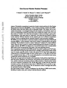
Unlike supervised learning, RL is a trial-and-error approach. The learning agent has to find which actions are the best without the help of a teacher, by trying them out. This process is called exploration. The quality and the speed of learning with finite data can depend dramatically on the agent’s exploration strategy. In MDPs with large or continuous state spaces, value functions can be represented by function approximators (e.g., CMACs or neural networks [17]). In that case, RL methods sample training data for the approximator, which consist of inputs (e.g., stateaction pairs) and targets (e.g., estimates of the action-value function). Equation (1) shows an example of inputs and targets for the SARSA algorithm. The approximator generalizes the value estimates gathered for a subset of the state-action pairs to the entire S A space. The interplay between the RL algorithm and the function approximator has an iterative, interleaved manner, as shown in Fig. 1. a subset of S 3 A
-.0/1 state-action values -.0/1 (targets) 2 2 RL 2 FA (inputs) 2
Q 4 s 5 a2 6
generalization of the value function to the entire S 3 A space
Fig. 1. Interaction of RL and FA learning
Function approximation in the context of RL is harder than in the classical, supervised learning setting. In supervised learning, many techniques assume a static training
set. In RL on the other hand, the estimates of the value function (which are the targets for the FA) evolve and improve gradually. Hence, the FA’s target function appears to be non-stationary. Moreover, the stochasticity in the environment and the exploration process may introduce variability into the training data (i.e., variability in the targets for a fixed input, which we will call “noise” from now on). To identify the potential sources of this noise, let us examine (1) again. Suppose that the same state-action pair � sˆ� aˆ � is encountered at time steps t1 and t2 during learning, and the FA is presented with the corresponding targets � rt1 � 1 ) γQ � st1 � 1 � at1 � 1 �7� and � rt2 � 1 ) γQ � st2 � 1 � at2 � 1 �7� . Table 1 shows four factors that can contribute to the noise. Note that these factors arise from the particular structure of the estimated value functions, from the randomized nature of the RL algorithm and, most of all, from the inherent randomness in the MDP. We will now introduce several attributes that help differentiate these sources of randomness, and quantify their effect. Factor 1: Factor 2: Factor 3: Factor 4:
Table 1. Factors contributing to the noise in the target of the FA training data. Stochastic immediate rewards 8:9 rt1 ; 1 8 < rt2 ; 1 Stochastic transitions: st1 ; 1 8 < st2 ; 1 8=9 rt1 ; 1 8 < rt2 ; 1 Q 4 st1 ; 1 5 at1 ; 1 6 8 < Q 4 st2 ; 1 5 at2 ; Stochastic transitions: st1 ; 1 8 < st2 ; 1 8=9 Different action choices: at1 ; 1 8 < at2 ; 1 8:9 Q 4 st1 ; 1 5 at1 ; 1 6 8 < Q 4 st2 ; 1 5 at2 ;
16 16
3 MDP Attributes We present six domain-independent attributes that can be used to quantitatively describe an MDP. For simplicity, we define them assuming discrete state and action spaces and availability of the MDP model. Later, we discuss how these assumptions can be lifted. State transition entropy (STE) measures the amount of stochasticity due to the environment’s state dynamics. Let Os a denote a random variable representing the outcome (next state) of the transition from state s when the agent performs action a. This variable takes values in S. We use the standard information-theoretic definition of entropy to measure the STE for a state-action pair � s � a � (as defined in [9]): ST E � s � a �>� H � Os a ���
+
∑ Psa s logPsa s
s ? S
(2)
A high value of ST E � s � a � means that there are many possible next states s (with Psa s A� @ 0) which have about the same transition probabilities. In an MDP with high STE values, the agent is more likely to encounter many different states, even by performing the same action a in some state s. In this case, state space exploration happens naturally to some extent, regardless of the exploration strategy used by the agent. Since extensive exploration is essential for RL algorithms, a high STE may be conducive to good performance of an RL agent. At the same time, though, a high STE will increase the variability of the state transitions. This suggests that the noise due to Factors 2 and 3 in Table 1 may increase, which can be detrimental for learning. The controllability (C) of a state s is a normalized measure of the information gain when predicting the next state based on knowledge of the action taken, as opposed to making the prediction before an action is chosen (note that a similar, but not identical, attribute is used by Kirman [9]). Let Os denote a random variable (with values from S)
representing the outcome of a uniformly random action in state s. Let A s denote a random variable representing the action taken in state s. We consider A s to be chosen from a uniform distribution. Now, given the value of As , information gain is the reduction in the entropy of Os : H � Os � + H � Os � As � , where H � Os ���
+
∑ Ps s logPs s
s S
H � Os � As ���
+
+ �
∑�
s S
∑
a A
1 A � �
∑ Psa s �
log �
a A
1 A � �
∑ Psa s �
a A
1 Psa s log � Psa s � ∑ A � � sB S
The controllability in state s is defined as: C � s ���
H � O s � + H � O s � As � H � Os �
(3)
If H � Os �C� 0 (deterministic transitions for all actions), then C � s � is defined to be 1. It may also be useful (see Sect. 5) to measure the forward controllability (FC) of a state-action pair, which is the expected controllability of the next state: FC � s � a ���
∑ Psa s C � s �
s S
(4)
High controllability means that the agent can exercise a lot of control over which trajectories (sequences of states) it goes through, by choosing appropriate actions. Having such control enables the agent to reap higher returns in environments where some trajectories are more profitable than others. Similar to the STE, the level of controllability in an MDP also influences the potential exploration of the state space. Because in a highly controllable state s the outcomes of different actions are quite different, the agent can choose what areas to explore. This can be advantageous for the RL algorithm, but may be detrimental for function approximation, because of the noise due to Factor 4 in Table 1. The variance of immediate rewards, V IR � s � a � , characterizes the amount of stochasticity in the immediate reward signal. High VIR causes an increase in the noise due to Factor 1 in Table 1, thus making learning potentially more difficult. The risk factor (RF) measures the likelihood of getting a low reward after the agent performs a uniformly random action. This measure is important if the agent has to perform as well as possible during learning. Let rsau denote the reward observed on a transition from a state s after performing a uniformly random action, a u . The risk factor in state s is defined as: RF � s ��� Pr � rsau D E � rsau � + ε � s �7� �
(5)
where ε � s � is a positive number, possibly dependent on the state, which quantifies the tolerance to lower-than-usual rewards. Note that low immediate rewards do not necessarily mean low long-term returns. Nevertheless, knowledge of RF may help minimize losses, especially during the early stages of learning. The final two attributes are meant to capture the structure in the state transitions. The transition distance, T D � s � a � , measures the expected distance between state s and its
successor states, according to some distance metric on S. We are currently investigating what distance metric would be appropriate. One candidate is a (weighted) Euclidean distance, but this is not adequate for all environments. The transition distance may affect RL when using global function approximators, such as neural networks. In the case of incremental learning with global approximators, training on two consecutive inputs that are very different may create mutual interference of the parameter updates and impede learning. Hence, such MDPs may benefit from using local approximators (e.g. Radial Basis Networks). The transition variability, TV � s � a � , measures the average distance between possible next states. With a good TV metric, a high value of TV � s � a � would indicate that the next states can have very different values, and hence introduce noise due to Factor 3 in Table 1. In continuous state spaces, the attributes are defined by using integrals instead of sums. If the model of the process is not available, these attributes can be estimated from the observed transitions, both for discrete and continuous state spaces. The attributes can be measured locally (for each state or state-action pair) or globally, as an average over the entire MDP. Local measures are most useful for tuning the parameters of the RL algorithm. For example, in Sect.5, we suggest how they can be used to adapt the exploration strategy. In the experiments presented in the next section, we use global measures - sample averages of the attribute values, computed under the assumption that all states and actions are equally probable. This choice of the sampling distribution is motivated by our intention to characterize the MDP before any learning takes place. Note, however, that under some circumstances, weighted averages might be of more interest (e.g., if we want to compute these attributes based on behavior generated by a restricted class of policies). If the sample averages were estimated on-line, during learning, they would naturally reflecting the state distribution that the agent is actually encountering.
4 Empirical Study In this section we focus on studying the effect of two of state-transition entropy (STE) and controllability (C), on the quality of the policies learned by an RL algorithm using linear function approximation. The work of Kirman suggests that these attributes influence the performance of off-line dynamic programming (DP) algorithms, to which RL approaches are related. Hence, it seems natural to start with studying these two attributes. Our experiments with the other attributes are still in their preliminary stages, and the results will be reported in future work. In Sect. 4.1 we present the application domains used in the experiments. The experimental details and the results are described in Sect.4.2. 4.1 Tasks In order to study empirically the effect of MDP characteristics on learning, it is desirable to consider a wide range of STE and C values, and to vary these two attributes independently. Unfortunately, the main collection of currently-popular RL tasks 1 contains only a handful of domains, and the continuous tasks are mostly deterministic. So 1
Reinforcement learning repository at the University of Massachusetts, Amherst www-anw.cs.umass.edu/rlr
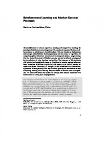
our experiments were performed on artificial random MDPs, as well as randomized versions of the well-known Mountain-Car task. Random discrete MDPs (RMDPs) have already been used for experimental studies with tabular RL algorithms. In this paper, we use as a starting point a design suggested by Sutton and Kautz for discrete, enumerated state spaces2 , but we extend it in order to allow feature-vector representations of the states. Fig. 2 shows how transitions are performed in an RMDP. The left panel shows the case of a discrete, enumerated state space. For each state-action pair � s � a � the next state s is selected from a set of b possible next states, according to the probability distribution Psa s � j � 1 � �"�E� � b. The reward is then j
sampled from a normal distribution with mean Ras s and variance Vsa s . Such MDPs are easy to generate automatically. s a s1'
sj'
s
Taken with P(s,a,sj')
sb'
s' r~N(R(s,a,s'),V(s,a,s'))
a N1
Nj
Taken with Pj(s,a)
Nb
v1~N(Mj1(s,a),Vj1(s,a))... vn~N(Mjn(s,a),Vjn(s,a)) s' r~N(R(s,a,s'),V(s,a,s'))
Fig. 2. Random MDPs
Our RMDPs are a straightforward extension of this design. A state is described by a feature vector: � v1 � �E�E� � vn �&� with vi � � 0 � 1� . State transitions are governed by a mixture of b multivariate normal distributions (Gaussians) N � µj � σj � , with means µj �F� µ1j � �G�H� µnj � and variances σj �I� σ1j � �H�G� σnj � . The means µij � M ij � s � a � and variances σij � V ji � s � a � are functions of the current state-action pair, � s � a � . Sampling from this mixture is performed hierarchically: first one of the b Gaussian components is selected according to probabilities Pj � s � a � � j � 1 � �H�G� b, then the next state s is sampled from the selected component, N � µ j � σ j � 3 . Once the next state s is determined, the reward for the transition is sampled from a normal distribution with mean R � s � a � s "� and variance V � s � a � s J� . The process may terminate at any time step according to a probability distribution P � s "� . Mixtures of Gaussians are a natural and non-restrictive choice for modeling multivariate distributions. Of course, one can use other basis distributions as well. We designed a generator for RMDPs of this form4 , which uses as input a textual specification of the number of state variables, actions, branching factor, and also some constraints on the functions mentioned above. In these experiments we used piecewise constant functions to represent Pj � s � a � � M ij � s � a � � V ji � s � a � � R � s � a � s E� and V � s � a � s E� , but this choice can be more sophisticated. Mountain-Car[17] is a very well-studied minimum-time-to-goal task. The agent has to drive a car up a steep hill by using three actions: full throttle forward, full throttle reverse, or no throttle. The engine is not sufficiently strong to drive up the hill directly, so 2 3 4
� www.cs.umass.edu/ rich/RandomMDPs.html By setting the variances σij to zero and using discrete feature values, one can obtain RMDPs with discrete state spaces. The C++ implementation of the RMDP � generator and the MDPs used in these experiments will be available from www.cs.mcgill.ca/ sonce/
the agent has to build up sufficient energy first, by accelerating away from the goal. The state is described by two continuous state variables, the current position and velocity of the car. The rewards are -1 for every time step, until the goal is reached. If the goal has not been reached after 1000 time steps, the episode is terminated. We introduced noise in the classical version of the Mountain Car task by perturbing either the acceleration or the car position. In the first case, the action that corresponds to no throttle remained unaffected, while the other two actions were perturbed by zero-mean Gaussian noise. This is done by adding a random number to the acceleration of +1 or -1. The new value of the acceleration is then applied for one time step. In the second case, the car position was perturbed on every time step by zero-mean Gaussian noise. 4.2 Effect of Entropy and Controllability on Learning We performed a set of experiments to test the hypothesis that STE and C have a statistically significant effect on the quality of the policies learned with finite amounts of data. We used a benchmark suite consisting of 50 RMDPs and 10 randomized versions of the Mountain-Car task (RMC). All the RMDPs had two state variables and two actions. In order to estimate the average STE and C values for these tasks, each state variable was discretized into 10 intervals; then, 100 states were chosen uniformly (independently of the discretization) and 150 samples of state transitions were collected for each of these states.5 The STE and C values were estimated for each of these states (and each action, in the case of STE) using counts on these samples. Then the average value for each MDP was computed assuming a uniform state distribution.6 The RMDPs formed 10 groups with different combinations of average STE and C values, as shown in the left panel of Fig. 3. Note that it is not possible to obtain a complete factorial experimental design (where all fixed levels of one attribute are completely crossed with all fixed levels of the other attribute), because the upper limit on C is dependent on STE. However, the RMDP generator allows us to generate any STE and C combination in the lower left part of the graph, up to a limiting curve. For the purpose of this experiment, we chose attribute values distributed such that we can still study the effect of one attribute while keeping the other attribute fixed. Note that each group of RMDPs contains environments that have similar STE and C values, but which are obtained with different parameter settings for the RMDP generator. The RMDPs within each group are in fact quite different in terms of state transition structure and rewards. The average values of STE and C for the RMC tasks are shown in the right panel of Fig. 3. We used two tasks with acceleration noise (with variances 0.08 and 0.35 respectively) and eight tasks with position noise (with variances 5 K 10 L 5 , 9 K 10 L 5 , 17 K 10 L 5 , 38 K 10 L 5, 8 K 10 L 4, 3 K 10 L 3 , 9 K 10 L 3 and 15 K 10 L 3). These tasks were chosen in order to give a good spread of the STE and C values. Note that for the RMC tasks, STE and C are anti-correlated. 5 6
Note that by sampling states uniformly, we may get more than one state in one bin of the discretization, or we may get no state in another bin. For the purpose of estimating STE and C beforehand, the choice of either uniform state distribution or the distribution generated by a uniformly random policy are the only natural choices. Preliminary experiments indicate that the results under these two distributions are very similar.
RMDPs
4
1.6
3.5
1.4
3
1.2
2.5
STE
STE
0.8
1.5
0.6
1
0.4
0.5
0.2
0
0.1 0.2 0.3 0.4 0.5 0.6 0.7 0.8 0.9 1
Controllability (C)
Position noise Acceleration noise
1
2
0
RMC Tasks
0
0
0.1 0.2 0.3 0.4 0.5 0.6 0.7 0.8 0.9
Controllability (C)
Fig. 3. Values of the Attributes for MDPs in the Benchmark Suite
We used SARSA as the RL algorithm and CMACs as function approximators [17] to represent the action-value functions. The agent followed an ε-greedy exploration strategy with ε � 0 � 01. For all tasks, the CMAC had five 9 9 tilings, each offset by a random fraction of a tile width. For the RMDPs, each parameter w of the CMAC architecture had an associated learning rate which followed a decreasing schedule αt � 1 M 25 0 M 5 � nt , where nt is the number of updates to w performed by time step t. For the RMCs, we used a constant learning rate of α � 0 � 0625. These choices were made for each set of tasks (RMDPs and RMCs) based on preliminary experiments. We chose settings that seemed acceptable for all tasks in each set, without careful tuning for each MDP. For each task in the benchmark suite, we performed 30 learning runs. Each run consisted of 10000 episodes, where each episode started in a uniformly chosen state. For the RMDPs, the termination probability was set to 0.01 for all states. Every 100 trials, the current policy was evaluated on a fixed set of 50 test states, uniformly distributed across the state space. The best policy on a particular run r is the one with the maximum average return (MARr ) over the states in the test set. The learning quality is measured as the average returns of the best policies found: LQ � ∑30 r � 1 MARr . Note that it is not always possible to compare the LQ measure directly for different MDPs, because their optimal policies may have different returns (thus the upper limits on MAR r and LQ are different). So we need to normalize this measure across different MDPs. Ideally, we would like to normalize with respect to the expected return of the optimal policy. Since the optimal policy is not known, we normalize instead by the average return of the uniformly random policy over the same test states (RURP). The normalized learning LQ quality (NLQ) measure used in the experiments is NLQ � RURP , if rewards are positive RURP (as is the case of the RMDPs), and NLQ � otherwise (for the RMCs). We conLQ ducted some experiments with RMDPs for which we knew the optimal policy and the results for the optimally and RURP-normalized LQ measures were very similar. Note that learning quality of RL algorithms is most often measured by the return of the final policy (rather than the best policy). In our experiments, the results using the return of the final policy are very similar to those based on the best policy (reported below), only less statistically significant. The within-group variance of the returns is much larger for the final policies, due to two factors. First, final policies are more affected by the learning rate: if the learning rate is too high, the agent may deviate from a good policy. Since the learning rate is not a factor in our analysis, it introduces unexplained variance. Secondly, SARSA with FA can exhibit an oscillatory behavior [5], which also
increases the variance of the returns if they are measured after a fixed number of trials. We plan to study the effect of the learning rate more in the future. To determine if there is a statistically significant effect of STE and C on NLQ, we performed three kinds of statistical tests. First, we used analysis of variance [2], to test the null hypothesis that the mean NLQ for all 10 groups of RMDPs is the same. We performed the same test for the 10 RMC tasks. For both domains, this hypothesis can be rejected at a significant confidence level (p D 0 � 01). This means that at least one of the two attributes has a statistically significant effect on NLQ. We also computed the predictive power (Hay’s statistic [2]) of the group factor, combining STE and C, on NLQ. The values of this statistic are 0.41 for the RMDPs and 0.57 for the RMCs. These values indicate that the effect of STE and C is not only statistically significant but also practically usable: the mean squared error in the prediction of the NLQ is reduced by 41% and 57% respectively for the RMDPs and RMC tasks, as a result of knowing the value of these attributes for the MDP. This result is very important because our longterm goal is to use knowledge about the attributes for making practical decisions, such as the choice of the algorithm or parameter settings for the task at hand. For the RMDP domains, the combination of STE and C values has the most predictive power (41%), whereas STE alone has only 4% prediction power and C alone has none. This suggests that both attributes have an effect on NLQ and should be considered together. Figure 4 shows the learning quality as a function of STE and C for the RMDPs (left panel) and for the RMC tasks (middle and right panels). Note that for the RMC tasks, we cannot study the effects of STE and C independently, because their values are anti-correlated. For ease of comparing the results to those obtained for RMDPs, we include two graphs for the RMC tasks, reflecting the dependency of NLQ on STE and C (middle and right panels of the figure 4). We emphasize that both graphs reflect one trend: as STE increases (and C decreases correspondingly), NLQ decreases. The reader should not conclude that STE and C exhibit independent effects in the case of the RMC tasks. As can be seen in the figure, for both domains (RMDPs and RMCs) the quality decreases as the entropy increases. We also conducted Least Significant Difference (LSD) tests [2] to compare the mean NLQ of the different pairs of RMDP groups and different pairs of RMC tasks. These tests (conducted at a conventional 0 � 05 confidence level), show that there is a statistically significant difference in the mean NLQ for all groups of RMDPs with different STE values, but the effect of STE becomes less significant as the value of the STE increases (potentially due to a floor effect). The trend is the same for the RMC tasks. As discussed in Sect. 3, high entropy is associated with the amounts of noise in the training data due to Factors 2 and 3 in Table 1, which makes learning more difficult. As we discussed in Sect. 2, the amount of noise also depends on the shape of the action-value functions. For example, if the actionvalue function is constant across the state-action space, then there will be no noise due to Factor 3 (see Table 1). Additional experiments with RMDPs that have relatively smooth and flat action-value functions7 showed that in this case, the learning quality increased as the STE increased. This is due to the positive effect of extensive statespace exploration in high-entropy MDPs. Thus, the effect of STE on learning quality 7
In those RMDPs, one action has higher rewards than the other in all states and the functions R 4 s 5 a 5 sNB6 have a small range.
RMDPs
1.5
16
1.45 1.4
STE~0.5
RMC Tasks
16
14
14
12
12
RMC Tasks
1.35
NLQ
10
10
1.3
NLQ
NLQ
1.25 1.2
8
8
6
6
4
4
1.15
STE~1.5 STE~3.5
1.1 1.05
0
0.2
0.4
0.6
Controllability (C)
0.9
2
2
0 0.25 0.37
STE
0.8
1.29 1.52
0.06 0.24
0.45 0.68 0.81
1
Controllability (C)
Fig. 4. Learning Quality
is a tradeoff between the negative effect of noise and the positive effect of natural state space exploration. The LSD tests also show differences in NLQ for the groups of RMDPs with different C values. The differences are significant between some of the groups with STE O 0 � 5 and STE O 1 � 5 levels. They appear when C changes by about 0.4. As can be seen from the left panel of Fig.4, the learning quality increases as controllability increases. As discussed in Sect. 3, high controllability means that the agent can better exploit the environment, and has more control over the exploration process as well.
5 Conclusions and Future Work In this paper, we proposed attributes to quantitatively characterize MDPs, in particular in terms of the amount of stochasticity. The proposed attributes can be either computed given the model of the process or estimated from samples collected as the agent interacts with its environment. We presented the results of an empirical study confirming that two attributes, state transition entropy and controllability, have a statistically significant effect on the quality of the policies learned by a reinforcement learning agent using linear function approximation. The experiments showed that better policies are learned in highly controllable environments. The effect of entropy shows a trade-off between the amount of noise due to environment stochasticity, and the natural exploration of the state space. The fact that the attributes have predictive power suggests that they can be used in the design of practical RL systems. Our experiments showed that these attributes also affect learning speed. However, statistically studying this aspect of learning performance is difficult, since there is no generally accepted way to measure and compare learning speed across different tasks, especially when convergence is not always guaranteed. We are currently trying to find a good measure of speed that would allow a statistically meaningful study. We are also currently investigating whether the effect of these attributes depends on the RL algorithm. This may provide useful information in order to make good algorithmic choices. We are currently in the process of studying the effect of the other attributes presented in Sect. 3. The empirical results we presented suggest that entropy and controllability can be used in order to guide the exploration strategy of the RL agent. A significant amount of research has been devoted to sophisticated exploration schemes (e.g., [11], [4], [12]).
Most of this work is concerned with action exploration, i.e. trying out different actions in the states encountered by the agent. Comparatively little effort has been devoted to investigating state-space exploration (i.e. explicitly reasoning about which parts of the state space are worth exploring). The E 3 algorithm [8] uses state-space exploration in order to find near-optimal policies in polynomial time, in finite state spaces. We are currently working on an algorithm for achieving good state-space exploration, guided by local measures of the attributes presented in Sect. 3. The agent uses a Gibbs (softmax) exploration policy [17]. The probabilities of the actions are based on a linear combination of the action values, local measures of the MDP attributes and the empirical variance of the FA targets. The weights in this combination are time-dependent, in order to ensure more exploration in the beginning of learning, and more exploitation later. Acknowledgments This research was supported by grants from NSERC and FCAR. We thank Ricard Gavald`a, Ted Perkins, and two anonymous reviewers for valuable comments.
References 1. Bertsekas, D. P., Tsitsiklis, J.N.: Neuro-Dynamic Programming. Belmont, MA: Athena Scientific (1996) 2. Cohen, P.R.: Empirical Methods for Artificial Intelligence. Cambridge, MA: The MIT Press (1995) 3. Dean, T., Kaelbling, L., Kirman, J., Nicholson, A.: Planning under Time Constraints in Stochastic Domains. Artificial Intelligence 76(1-2) (1995) 35-74 4. Dearden, R., Friedman, N., Andre, D.: Model-Based Bayesian Exploration. In Uncertainty in Artificial Intelligence: Proceedings of the Fifteenth Conference (UAI-1999) 150-159 5. Gordon, J.G.: Reinforcement Learning with Function Approximation Converges to a Region. Advances in Neural Information Processing Systems 13 (2001) 1040-1046 6. Hogg, T., Huberman, B.A., Williams, C.P.: Phase Transitions and the Search Problem (Editorial). Artificial Intelligence, 81 (1996) 1-16 7. Hoos, H.H., Stutzle, T. : Local Search Algorithms for SAT: An Empirical Evaluation. Journal of Automated Reasoning, 24 (2000) 421-481. 8. Kearns, M., Singh, S.: Near-Optimal Reinforcement Learning in Polynomial Time. In Proceedings of the 15th International Conference on Machine Learning (1998) 260-268 9. Kirman, J.: Predicting Real-Time Planner Performance by Domain Characterization. Ph.D. Thesis, Brown University (1995) 10. Lagoudakis, M., Littman, M.L. : Algorithm Selection using Reinforcement Learning Proceedings of the 17th International Conference on Machine Learning (2000) 511-518. 11. Meuleau, N., Bourgine, P.: Exploration of Multi-State Environments: Local Measures and Back-Propagation of Uncertainty. Machine Learning 35(2) (1999) 117-154 12. Moore, A.W., Atkeson, C.G.: Prioritized Sweeping: Reinforcement Learning with Less Data and Less Time. Machine Learning, 13 (1993) 103-130 13. Papadimitriou, C.H., Steiglitz, K: Combinatorial Optimization: Algorithms and Complexity. Prentice Hall (1982) 14. Papadimitriou, C.H., Tsitsiklis, J.N.: The Complexity of Markov Chain Decision Processes. Mathematics of Operations Research 12(3) (1987) 441-450 15. Puterman, M.L.: Markov Decision Processes: Discrete Stochastic Dynamic Programming. Wiley (1994) 16. Singh, S.P., Jaakkola, T., Jordan, M.I.: Reinforcement Learning with Soft State Aggregation. Advances in Neural Information Processing Systems, 7 (1995) 361-368 17. Sutton, R.S., Barto, A.G.: Reinforcement Learning. An Introduction. Cambridge, MA: The MIT Press (1998)