Characterizing Spatial Pattern and Heterogeneity of Pine ... - DukeSpace

Characterizing Spatial Pattern and Heterogeneity of Pine Forests in North Carolina’s Coastal Plain using LiDAR

By Lindsey Smart Advisor: Dr. Jennifer Swenson May 2009

Masters project submitted in partial fulfillment of the requirements for the Master of Environmental Management degree in the Nicholas School of the Environment and Earth Sciences of Duke University 2009

Characterizing Spatial Pattern and Heterogeneity of Pine Forests in North Carolina’s Coastal Plain using LiDAR ____________________________________________________________________________________________

ABSTRACT Forest ecosystems are often characterized by their spatial pattern, structure, and heterogeneity. A significant portion of the variability and texture within forests can be attributed to the heterogeneity of a forest’s canopy structure. Canopy structure influences important forest processes, which in turn, influence associations between animals and these particular forested habitats. Methods for quantifying these aspects of forest structural components exist, but have been largely unexplored for broad extents. Thus, remote sensing tools that directly characterize these attributes of habitat structure would be beneficial for management activities and conservation planning. LiDAR (Light Detection And Ranging) is such a tool, as an active remote sensing technology that provides fine-grained information about the three-dimensional structure of ecosystems across a broad spatial extent. This project assesses the feasibility of using the state-wide North Carolina Floodplain Mapping LiDAR dataset to differentiate between the structural components of evergreen forest types in North Carolina’s coastal plain. Vertical structure and spatial patterns of vertical structure were quantified using geospatial measures such as semivariogram/ correlograms, lacunarity analysis, and correlation length. LiDAR-derived metrics were also created for comparison with standard fieldbased measurements of stand structure. I found that LiDAR is capable of measuring canopy variation and can differentiate between the structural characteristics of evergreen forest types. Also, the N.C. LiDAR has potential for use as a surrogate for field measurements when collection is not feasible due to time, labor, or financial constraints. In addition, the project examined LiDAR’s use as a screening tool in the identification of suitable habitat for the federally endangered red-cockaded woodpecker (Picoides borealis). I used Maximum Entropy (Maxent), an inductive modeling algorithm for presence data only, to create a spatial species distribution model using LiDAR-derived variables in addition to more typical geospatial variables. The Area (AUC) under the Receiver Operating Characteristic (ROC) curve was analyzed for increases in predictive power with additions of variables. Results suggested that the addition of LiDAR-derived variables to habitat models improved their predictive power, resulting in a test AUC increase from 0.923 with standard spatial variables only, to a test AUC of 0.951 with LiDAR-derived variables added. This analysis is believed to be one of the first to explore the Floodplain Mapping LiDAR dataset for characterizing forest structural characteristics in North Carolina’s coastal plain in an attempt to assess its potential for application in broad scale wildlife habitat analyses. The success of this project has important implications for natural resource management and conservation planning, especially given that the LiDAR dataset is publicly available and covers the entire state of North Carolina.

___________________________________________________________________________

i


ACKNOWLEDGEMENTS I would like to thank the numerous faculty members here at the Nicholas School of the Environment, for the wonderful educational experience. In particular, I would like to thank my advisor, Dr. Jennifer Swenson for her patience, optimism, and guidance during my two years here at the Nicholas School. Many thanks and much appreciation for Dr. Norm Christensen, without whom, this project would not have been feasible. I would also like to thank Dr. Dean Urban, Joe Sexton, and Pete Harrell for all their help and for lending an ear when I needed it. I would also like to thank Mr. and Mrs. Fred Stanback for allowing the wonderful opportunity to work at the North Carolina Coastal Land Trust this past summer. I am also very grateful for the guidance and mentoring that Mrs. Janice Allen, my internship supervisor, gave me at the Coastal Land Trust. Her enthusiasm about conservation is responsible for sparking my interest in the longleaf pine ecosystem within North Carolina’s coastal plain. To Ryan, in appreciation of his patience and support. Finally, to my parents, Jim and Sue, for their unconditional love and support in all my endeavors.

___________________________________________________________________________ ii


Table of Contents 1.0 INTRODUCTION……………………………………………………………... 1 1.1 Overview of LiDAR…………………………………………………………...

2

1.1.1 LiDAR in Stand-Based Assessment Studies……………………………..

4

1.1.2. LiDAR in Habitat Modeling Studies……………………………………

5

2.0 PHYSICAL LOCATION & ECOLOGICAL CONTEXT…………………… 7 2.1. U.S. Marine Corps Base Camp Lejeune …………………………………… 7 2.1.1. Forest Stand Management at Camp Lejeune…………………………... 8 2.2. Longleaf Pine Savannas & Red-cockaded Woodpeckers…………………. 10 3.0 STUDY GOALS…………………………………………………………………

11

3.1. Study Objectives……………………………………………………………... 11 4.0 MATERIALS & METHODS…………………………………………………..

12

4.1. Study Area……………………………………………………………………. 13 4.1.1. Forest Stand Locations…………………………………………………

13

4.1.2 Habitat Suitability Analysis Study Location…………………………….

14

4.2 LiDAR Data…………………………………………………………………..

15

4.2.1. Raw Point Clouds………………………………………………………. 16 4.3. Descriptive Analyses of Vertical Structure…………………………………. 18 4.3.1. Semivariograms/ Correlograms………………………………………... 18 4.4. LiDAR-derived Forest Metrics……………………………………………...

18

4.4.1. Coefficient of Variation………………………………………………… 19 4.4.2. Canopy Height Models…………………………………………………. 19 4.4.3. Canopy Cover…………………………………………………………..

20

4.4.4. Height Profiles………………………………………………………….

20

4.5. Spatial Pattern Analysis………………………………………......................

21

4.5.1 Lacunarity Analysis……………………………………………………..

21

4.5.2. Correlation Length……………………………………………………... 23 4.6 Correlations & Regression Analyses………………………………………...

24

4.7. Case Study: RCW Habitat Suitability Analysis ……………………………. 25 5.0 RESULTS ………………………………………………………………………. 29

___________________________________________________________________________ iii


5.1. Statistical Summary Measures of Structural Characteristics………………

29

5.2. Descriptive Analyses of Vertical Structure ………………………………… 32 5.2.1 Variograms/ Correlograms……………………………………………... 32 5.3. LiDAR-derived Forest Metrics ……………………………………………..

32

5.3.1 Height Variability – Mean, Maximum, & CV…………………………...

32

5.3.2. Canopy Cover Estimates & Canopy Height Profiles…………………... 33 5.3.2.1 Canopy Cover…………………………………………………...

33

5.3.2.2. Height Profiles…………………………………………………..

34

5.4. Spatial Pattern Analysis……………………………………….................….

35

5.4.1. Lacunarity Analysis…………………………………………………….. 35 5.4.2. Correlation Length……………………………………………………... 37 5.5. LiDAR Comparisons with Field-based Measurements……………………

37

5.6. Case Study: RCW Habitat Suitability Analysis…………………………….

40

6.0 DISCUSSION…………………………………………………………………...

46

7.0 IMPLICATIONS FOR MANAGEMENT & CONSERVATION…………..

49

8.0 CONCLUSION..………………………………………………………………..

50

REFERENCES………………………………………………………………….

51

APPENDICES ………………………………………………………………….. 55-72

___________________________________________________________________________ iv


List of Tables & Figures

________

Figure 1: Physical Location………………………………………………………………… 7 Figure 2: Image of Red-cockaded Woodpecker…………………………………………... 10 Figure 3: Study Site Locations.……………………………………………………………..

14

Figure 4: Habitat Suitability Analysis Study Site Location……………………………….

15

Figure 5: LiDAR Raw Point Clouds………………………………………………………..

17

Table 1: Input Environmental Variables for Habitat Modeling………………………….. 26 Figure 6: Longleaf/Loblolly Pine LiDAR Height Density Distributions………………..

31

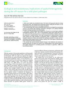
Figure 7: Longleaf/Loblolly Pine Height Profile Distributions………………………….

34

Figure 8: Log-Log Plot of Lacunarity vs. Box Size………………………………………..

36

Table 2: Correlation Matrix for Field Measures, RCW Sites, & LiDAR Metrics………... 38 Figure 9: Observed-Predicted Plot for Basal Area Predictions…………………………...

39

Table 3: Variables Used in Pine Basal Area Prediction…………………………………... 39 Table 4: Correlation Matrix for Continuous Environmental Variables Used in Maxent

40

Table 5: Heuristic Estimates of Percent Contribution to Model Training Algorithm…

42

Table 6: Jackknife Results for Environmental Variables Used in Maxent Model………

42

Table 7: Environmental Variables’ Ranked Averages in Maxent Model………………...

43

Table 8: AUC & Gain for Standard Variables Plus Addition of GAP/LiDAR/NDVI….

43

Figure 10: RCW Species Distribution Model……………………………………………… 45

___________________________________________________________________________

v


1.0 INTRODUCTION Differences in forest canopies, as expressed by their spatial heterogeneity and texture, can help distinguish between different forest types. These differences that help distinguish between forest types are also those that contribute to characteristic habitat types for wildlife. Thus, the structural components of forest canopies potentially influence associations between animals and these forested habitats. These dynamic three-dimensional components of forests are important because they provide information on canopy patterns that influence broader ecological patterns and processes. Methods for quantifying these aspects of forest canopy structure exist, but have been largely unexplored for many areas. Newer methods in remote sensing will greatly enhance the ability to explore and summarize these canopy patterns and create the opportunity for comparisons between diverse structural characteristics exhibited by different forest types. Remotely-sensed imagery has been an extremely beneficial tool in the development of habitat models and site prioritization efforts, but the majority of this imagery provides information only about two-dimensional characteristics despite the fact that habitat models would benefit greatly from the addition of broad-scale three dimensional structural characteristics. Passive optical imagery provides extensive information of generalized forest structural classes in the horizontal plane but is relatively insensitive to variation in forest canopy height. LiDAR (Light Detection and Ranging) is a remote sensing tool that can provide fine grain information about three-dimensional structures at broad scales, allowing for the replacement of labor-intensive field measurements, and the improvement of habitat modeling for species management and conservation. Canopy height and tree heights are key forest structural components that serve as indicators of forest composition and development stage, and more broadly, habitat quality. For most basic assessments, differences in stands and stand development have been reflected in mean and maximum heights of individual trees within the stand (Lefsky et al., 1999). But, even for stands with similar mean and maximum heights, there are more subtle differences in canopy structure elements that help differentiate between relatively similar stand compositions and development stages. Most previous estimates of tree heights and canopy structure have been gathered from field observations.

___________________________________________________________________________

1


Field observations for small stands pose no difficulty, but efforts to collect broad-scale field measurements accurately are time consuming, labor intensive, and costly. The application of LiDAR can provide fine-scale information across broad spatial extents, thus providing an excellent source of data for forest management. The ability to characterize the vertical structure of forests accurately has the potential to serve in a wide variety of forestry applications. For example, it can aid in the determination of stand dynamics and development, the distribution and estimation of canopy fuels, as well as provide important biomass and above ground carbon estimations. Therefore, the addition of LiDAR as a tool in forest management can be beneficial in many ways. With accurate estimations of forest stand dynamics and development stage characteristics, there is potential for extending the application of LiDAR to habitat suitability analyses for animal species that are dependent on the vertical structure of forests, which would greatly improve methods of ecological modeling for these species. The spatial extent of LiDAR availability varies, but some region-wide acquisitions have recently become available. In fact, LiDAR data has been acquired across the entire state of North Carolina via the North Carolina Floodplain Mapping Program and has been made publicly available (data downloads are available at http://lidar.cr.usgs.gov ). The available LiDAR information across the state provides us with the opportunity to characterize vegetation structural components at very broad scales. The goal of this project is to evaluate the feasibility of using the North Carolina LiDAR dataset, of which the capabilities have been largely unexplored, to characterize different evergreen forest types. I will examine the degree to which LiDAR-derived metrics can successfully differentiate between different evergreen stand types based on a complete dataset of multiple LiDAR returns. In addition, the project examines the potential for use of LiDAR in habitat suitability analyses for the federally endangered red-cockaded woodpecker (Picoides borealis) in North Carolina’s coastal plain. 1.1. Overview of LiDAR Until the late 1990’s, the majority of forest characterization was based on two-dimensional analyses of remotely sensed images (Vierling et al., 2008). The derivation of forest structure metrics and the modeling of these metrics from LiDAR point data can serve as a beneficial tool for forest

___________________________________________________________________________

2


inventory and for implementation in habitat characterization for suites of species greatly influenced by the structural components of forests. LiDAR contains a series of components within a system used to record elevational data. Key components include the IMU (inertial mapping unit to record pitch, roll and yaw), a GPS, a laser of a specified wavelength, and an on-board computer (USGS, 2007). The laser system, usually aboard an aircraft, fires a pulse and the pulse traverses through the terrain and is reflected, returning the pulse to the system. The basic measurement made by a LiDAR device is the distance between the sensor and a target surface, obtained by determining the elapsed time between the emission of a laser pulse and the arrival of the reflection of that pulse at the sensor’s receiver. Multiplying this time by the speed of light results in a measure of round trip distance and dividing the measure by two yields the distance between the sensor and the target. The surface of interest is repeatedly measured along a transect and the resulting information is an outline of both the ground surface and any vegetation obscuring it. There are many types of LiDAR sensors with variations in platform type, system type (e.g. profiling or scanning), type of pulse emitted (e.g. single, multiple or waveform), the size of the laser footprint, and the density of the postings, or returns on the ground (USGS, 2007). A scanning LiDAR system uses a scanning mirror to collect a swath of data underneath the aircraft. This system collects many more points underneath the aircraft and allows for overlapping flight lines which can help correct systematic errors. Multiple return systems allow more than one x, y, z (easting, northing, and elevation) coordinate per pulse, and as a result, there is a better chance for detecting the ground underneath vegetation canopies. Scanning LiDAR systems that record multiple returns are the systems that most commercial vendors currently use. Alternatively, a waveform return system records a continuous waveform of the energy returned per pulse which can provide a large amount of information. Currently this technology is being used in a research capacity by NASA, and is not available commercially. The size of the beam footprint can be different as well, with traditionally large footprints ranging from 10-25 m in diameter. Posting density is the spacing of the returns on the ground. Because this is not a regular pattern, posting density is usually measured as an average per unit area (e.g., 1 point per m2). The posting density is a function of the laser pulse rate, the flying height and speed of the aircraft, and the scan angle (USGS, 2007).

___________________________________________________________________________

3


The N.C. Floodplain Mapping Program data were collected between 2000 and 2003 in response to damages incurred by Hurricane Floyd in North Carolina. LiDAR data were collected in an effort to create updated digital elevation models (DEMs) for more accurate flood hazard mapping and floodplain management. The goal was to create DEMs for all of North Carolina using last return data from LiDAR (NC Floodplain Mapping Program, 2003). To favor the collection of “bare earth” data for DEM creation, the LiDAR data were collected during leaf-off conditions, so as to avoid interception of the laser profile by leaves on deciduous trees. The LiDAR data were collected using a platform aboard an aircraft operated by a commercial vendor. Because the goal of the N.C. Floodplain Mapping Program was the creation of DEMs derived only from bare earth data or ground returns (the returns arriving back to the aircraft platform last), the other returns representing other three-dimensional landscape characteristics were not used in the program. The accuracy of these other LiDAR returns and their applicability in various ecological analyses has not been adequately explored. Because LiDAR has the potential for use in a variety of applications, including the characterization of forest structure, an in-depth analysis of this LiDAR dataset is needed. 1.1.1. LiDAR in Stand-based Assessment Studies LiDAR can be used to derive forest structural components such as canopy height, canopy surfaces, maximum height, individual tree isolation, canopy closure, and tree density measures. Manufacturers and data providers report absolute elevation accuracies of 15 cm and even better relative accuracies (Lefsky et al., 2002). Accurate measures of tree and canopy height remain a primary attribute for forest inventories. Several studies have shown the benefit of using LiDAR for forest assessments, in terms of its applicability and its accuracy. At the stand level, measures such as mean tree height and diameter, timber volume, stem number, and canopy closure have been modeled using LiDAR-based estimates from discrete return small footprint LiDAR data. This typically involves regression-based methods in which percentiles of the distribution of canopy height measurements are used to predict forest characteristics within a spatial sampling frame based on empirical relationships (Hill, 2007). When the density of laser returns is greater than 5-10 per m2, individual tree-based estimates have been calculated providing even more accurate measurements than the ones mentioned above. Hall et al. (2005) estimated forest stand variables such as stand height, total above ground biomass, foliage biomass, basal area,

___________________________________________________________________________

4


and others for a fire prone ponderosa pine forest in Colorado using discrete-return LiDAR measurements. Observed versus predicted values of stand structure variables were highly correlated, with R2 values ranging from 57% to 87%. The most parsimonious linear models for biomass structure variables explained between 35% and 58% of the observed variability. Sherrill et al. (2008), used LiDAR from a discrete return system in The Fraser Experimental Forest in Colorado to approximate field-based measures of evergreen forest height and obtained an RMSE of less than 1 m. Bradburry et al. (2005) stated that LiDAR estimates explained 86% of the variation in canopy density index and so could be used as a surrogate for the field-based estimates of canopy density. Sexton et al. (2009) used a LiDAR dataset from the N.C. Floodplain Mapping Program for an analysis of LiDAR-based tree height accuracies in the Piedmont of North Carolina, specifically the Duke Forest. Results confirmed the discrete-return N.C. Floodplain LiDAR’s ability to measure canopy height in coniferous forests, using comparisons with field data (R2 = 0.86, RMSE 4.73 m). Therefore, the LiDAR dataset studied produced reasonable and consistent depictions of canopy heights for evergreen forest stands in North Carolina’s Piedmont. Using a larger and more robust sample size of forest stands, Hudak et al. (2006) substantiated other study results by suggesting that field-measured stand attributes such as mean stand height, tree density, and basal area were significantly correlated with LiDAR estimates in conifer forests. In this study, the variables most useful for predicting basal area were LiDAR height variables and the variable most useful for tree density calculation was canopy closure. Study results agree that some forms of LiDAR may be an accurate replacement for field-based observations and measurements for forest stand structural components. Having large-scale measures of forest structure, researchers can develop landscape-level analyses of important aspects of forests. 1.1.2. LiDAR in Habitat Modeling Studies With the proven ability of LiDAR data, a few studies have examined the applications of LiDAR for habitat modeling, both in a predictive sense and as an exploratory tool. Nelson et al. (2005) used LiDAR in conjunction with other sampling methods as a screening tool to locate potential habitat for the Delmarva fox squirrel (Sciurus niger cinereus). Broughton et al. (2006) used airborne LiDAR data to examine differences in the structural components between habitat and non-habitat for the marsh tit (Poecile palustris). Results showed striking differences between those areas ___________________________________________________________________________

5


occupied by the bird and those areas that were unoccupied. A statistical difference of 1.6m (13%) was found between occupied territories and non-occupied territories, with the occupied areas having a significantly higher proportion of tall trees because marsh tit habitat preference is for mature deciduous woodlands. Goetz et al. (2007) used several different remotely-sensed imagery techniques to assess optimal areas of heterogeneity for bird species richness in the Patuxent National Wildlife Refuge, Maryland. They created models with all variables (optical and LiDAR fusion), with LiDAR variables alone, and with optical variables alone. Canopy vertical distribution information was consistently found to be the strongest predictor of species richness. The LiDAR metrics were also consistently better predictors than traditional remotely sensed variables such as canopy cover. Graf et al. (2008), performed a similar analysis for a forest-dwelling species of grouse (Tetrao urogallus) in the Alps. The final habitat suitability model included habitat explanatory variables from both LiDAR and from passive sensors. This mixed model had higher predictive power than the model with LiDAR variables alone (AUC=0.71 for LiDAR alone and AUC= 0.77 for the mixed model). Relative tree canopy cover, derived from LiDAR, was the most important LiDAR-derived variable, with intermediate values indicating highest habitat suitability. The results suggested that LiDAR can improve habitat distribution models and allowed for the integration of individual habitat preferences at the scale of entire populations. These studies provide confirmation that LiDAR can be an important tool in habitat modeling fore certain species given that it is capable of distinguishing between a species’ preferred habitat and non-habitat. Because LiDAR provides a combination of fine resolution data and broad spatial extent with better vertical resolution and sampling density than can be achieved in the field, it can provide information on previously unmeasured habitat. It thus holds great promise for determining associations between species and vertical structure within forests.

___________________________________________________________________________

6


2.0 PHYSICAL LOCATION & ECOLOGICAL CONTEXT 2.1. U.S. Marine Corps Base Camp Lejeune The area of interest for this study was the United States Marine Corps Base Camp Lejeune located in Jacksonville, North Carolina (Figure 1).

Figure 1: General location of the U.S. Marine Corps Base Camp Lejeune in Jacksonville, NC.

Camp Lejeune lies within the White Oak River Basin in Onslow County and boasts habitat for several federally listed endangered, threatened, and rare species including the red-cockaded woodpecker. Because Camp Lejeune provides habitat for these species, the military installation is

___________________________________________________________________________

7


required by the Endangered Species Act (1973) to protect these species and to do so, the base performs extensive management activities to maintain the natural habitat (USMBC Camp Lejeune, 2006). In addition, in order to continue military training operations on the installation, they must ensure that no adverse effects to these species occur. Therefore, the environmental management division at Camp Lejeune has performed extensive inventories of forest stands, mapped locations of endangered species, and enhanced habitat in areas where the species are located (USMCB Camp Lejeune, 2006). As a result, Camp Lejeune serves as an excellent study site because of the wide variety and extensive inventory of evergreen forest types on their managed lands. It thus provides a significant site to test LiDAR-derived metrics and their ability to differentiate various forest structural components and preferred habitat types of the RCW. Camp Lejeune owns about 38,445 ha within the southern Atlantic Coastal Plain (USMCB Camp Lejeune, 2006). The federal government has dual responsibilities on these military installations, one to maintain the capacity for military training and operation and another, to serve as manager for the natural resources under its control. Much planning goes into endangered species management to ensure sustainable training lands (USMCB Camp Lejeune, 2006). Forest stand management is an important aspect of maintaining the ecological integrity at Camp Lejeune, particularly the restoration of forest stands to their more natural and historic communities of longleaf pine (Pinus palustris). 2.2.1. Forest Stand Management at Camp Lejeune Longleaf pine ecosystems were historically an integral part of the southeastern portion of North Carolina. In fact, they occurred throughout the majority of the southeast. After years of fire suppression and urban development, only 3% of the original longleaf pine savannas are present today (U.S. Fish and Wildlife Service, 2003). Longleaf pine ecosystems are important habitat for several rare, threatened, or endangered species, the most recognizable of these species being the redcockaded woodpecker. Interestingly, the majority of longleaf pine savannas tend to occur on federal lands, especially on military installations because they are managed with frequent prescribed burns, thus simulating the most natural state of the longleaf pine ecosystem. Because these installations provide some of the last relatively intact longleaf pine ecosystems in the southeast, they also tend to attract rare and endangered species.

___________________________________________________________________________

8


Camp Lejeune has an aggressive program to re-establish the natural longleaf pine savannas within their historic range, because of their importance to endangered species, especially the redcockaded woodpecker and because of their importance in wildland fire management and training operations. They continue to restore longleaf communities in sites within their historic range and habitat type. Forest stand management at Camp Lejeune includes the restoration of suitable forests to longleaf pine ecosystems to meet criteria for red-cockaded woodpecker habitat and for ease in training/ military operations. The goal of the management is to create low density pine stands, with mature longleaf as the dominant canopy tree species (USMCB Camp Lejeune, 2006). Therefore, the forest stands at Camp Lejeune vary in species composition and structure. This variety will prove useful in analyzing LiDAR’s ability to differentiate variations in canopy structure among various forest types. An essential factor that affects the structure and composition of forest types throughout the entire ecosystem is fire, and prescribed burns play an integral role in the management for historical longleaf pine ecosystems at Camp Lejeune. Without fire, development of shrub and mid-story levels truncate pine regeneration and these vegetation changes resulting from fire exclusion have a large impact on faunal communities, especially avian species. Fire, wind, and lightning are common disturbances that shape the structure and composition of longleaf forests (USMCB Camp Lejeune, 2006). All forests develop heterogeneous spacing resulting from disturbances and fire regimes. The spacing of trees and patches of trees is important for bird species that forage in open spaces within forests as well as for the development of groundcover. Areas that are not currently managed and those that do not experience appropriate fire return intervals, may become inundated with a thick midstory, can experience competition between pines and hardwoods, and overall provide less suitable habitat for avian species that search for more open foraging or nesting habitat. Also, the lack of fire and natural disturbances allows other species to encroach upon and out-compete the longleaf pine for its natural habitat. The stands at Camp Lejeune are in various stages of management; some are characteristic of the historic longleaf communities and others have had less management, and are dominated by off site species such as hardwoods or loblolly pines (Pinus taeda). The goal of current forest management plans is to clearcut sites with off-site species and re-plant with longleaf seedlings on

___________________________________________________________________________

9


those sites that historically grew longleaf pines. LiDAR is used in this analysis to distinguish between various structural components common in stands that are managed differently. The two different stand types considered are: stands managed extensively for mature longleaf pine and those stands that have yet to undergo management and typically are characteristic of a dominant loblolly pine overstory, an extensive hardwood midstory, and overall denser distributions of pines. 2.2. Longleaf Pine Savannas & Red-cockaded Woodpeckers Evergreen pine forests are important habitat for a suite of species, including the redcockaded woodpecker (Figure 2). Preferred habitat of the RCW is open pine woodlands and savannas with large old pines for nesting and roosting habitat. Large old pines are required as cavity trees because the trees are excavated completely within inactive heartwood, so that the cavity interior remains free from resin that can entrap birds (U.S. Fish and Wildlife Service, 2003). Cavity trees must be in open stands with little or no hardwood midstory and few or no hardwood overstory trees. Hardwood encroachment resulting from fire suppression is an issue and leads to less than optimal habitat for the RCW. RCWs also require a significant amount of foraging habitat which consists of mature pines

Figure 2: Red-cockaded woodpecker (PhotoSource: www.lejeune.usmc.mil)

with an open canopy, low density of small pines, little or no hardwood or pine midstory, few or no overstory hardwoods, and abundant native bunchgrass and forb groundcovers. Limiting factors for RCWs impact the persistence of breeding groups and include fire suppression, lack of cavity trees due to hardwood encroachment, and fragmentation due to anthropogenic influences (U.S. Fish and Wildlife Service, 2003).

___________________________________________________________________________ 10


Longleaf pine ecosystems, of primary importance to RCWs, are now among the most endangered systems on earth. Southern pine forests today are very different from the historic ecosystems that once dominated the southeast. Original pine forests were old, open, and contained a structure represented by two layers, a canopy and a diverse herbaceous groundcover. Forests dominated by loblolly pine were restricted to a portion of the southern Arkansas area, a portion of Virginia, and the very northeastern portion of North Carolina. Today, much of the forest is young, dense, and dominated by loblolly pine, with a substantial hardwood component and little or no herbaceous groundcover (U.S. Fish and Wildlife Service, 2003). Therefore, efforts to quantify the spatial pattern of these forest types and differences in structure between longleaf pine savannas and other forest types are important for a variety of reasons, especially in efforts to re-establish or restore this ecosystem back into areas that were part of the historic range.

3.0 STUDY GOALS The primary goal of this analysis is to provide an impetus for the application of the N.C. Floodplain Mapping Program LiDAR dataset in conservation and management projects by providing evidence supporting its use as a tool for characterizing forest structural components at both fine and broad scales. To support the claim that LiDAR can be useful and beneficial in a variety of applications, the capability of the N.C. LiDAR dataset to measure structural variation was examined using USMCB Camp Lejeune in North Carolina’s coastal plain as a test site. 3.1. Study Objectives The following objectives were set in order to fulfill the above-mentioned study goals: •

Assess the feasibility of using LiDAR to differentiate between the canopy structures of various evergreen forest stands in the coastal plain of North Carolina by: 1. Comparing within- and between- stand variability in vertical structure among general types. 2. Creating LiDAR-derived metrics of forest structure for comparisons with field data. 3. Analyzing scale-dependent measures of horizontal spatial patterns derivable from LiDAR.

___________________________________________________________________________ 11


•

Examine the potential of future use of LiDAR data in red-cockaded woodpecker habitat suitability analyses in the coastal plain by: 1. Examining associations between RCW occurrences and LiDAR-derived metrics. 2. Examining associations between RCW occurrences and measures of horizontal spatial pattern. 3. Testing the performance of LiDAR-derived variables in a habitat suitability analysis. for RCWs in a sub-basin of the White Oak River Basin, within the coastal plain of North Carolina.

4.0 MATERIALS & METHODS N.C. LiDAR were acquired and processed for the New River sub-basin within the White Oak River Watershed in North Carolina. A set of finer-scale sites with various forest structures were selected within the portion of the sub-basin where Camp Lejeune is located. The distributions of LiDAR heights were used to examine patterns of vertical and horizontal structure. The data were analyzed with exploratory data analysis, semivariogram/correlogram analysis, and lacunarity analysis. LiDAR-derived metrics were created for the plots and included maximum height, mean height, standard deviation, coefficient of variation, lacunarity statistic, overstory correlation length, understory correlation length and canopy cover. These metrics were compared to field data collected at each of the fourteen stands, and the value of these metrics for predicting preferred RCW habitat was also analyzed. LiDAR data were processed using the LiDAR export utility EdBex (Version 1.06, 2002). LiDAR manipulation and geospatial analyses were performed using ArcGIS Version 9.3 (ESRI, Redlands, CA), ArcScene for the three-dimensional viewing of geospatial data, and Hawth’s Tools, an extension of Arc GIS Version 9.3 (Beyer, H. L. 2004). Landscape metrics were generated in QRULE (extension of RULE, Gardner, 1999) and FragStats (Version 3.3 Build 4, 2002). Species distribution models were generated using Maxent (Version 3.2.19, 2006). All statistical analyses were performed using R statistical computing software (R Development Core Team, 2008).

___________________________________________________________________________ 12


4.1. Study Area

4.1.1. Forest Stand Locations To analyze the effectiveness of LiDAR-derived forest metrics as screening tools for different structural types, 14 forest stands within Camp Lejeune’s installation area were selected (Figure 3) from all inventoried stands on the base. U.S Marine Corps Camp Lejeune maintains an extensive inventory of all managed and unmanaged stands. As part of the Carolina Vegetation Survey, vegetation surveys and tree stand data were collected at several 0.1 ha plots within some of the longleaf dominant forest stands and a GPS point location was recorded at the center of these plots. Another survey dataset was used for stand selection and consisted of GPS point locations of loblolly dominated 0.1ha plots (US Marine Corps Base Camp Lejeune, Natural Resource Management Division, unpublished data).Two stand types were sampled and represented by these vegetation survey points: stands dominated by mature longleaf pines and stands dominated by loblolly pines having an extensive hardwood midstory. Seven point locations were randomly selected from the Carolina Vegetation Survey dataset and seven point locations were randomly selected from Camp Lejeune’s personal dataset to obtain point locations of each forest type. A buffered 1 ha square on each random point was created for all 14 point locations. The resultant dataset included 14 1 ha plots, 7 with longleaf pine as the dominant tree species and 7 with loblolly pine as the dominant species. These plots will hereafter be referred to as longleaf pine plots and loblolly pine plots.

___________________________________________________________________________ 13


Figure 3: Study site locations and locations of loblolly/ longleaf pine within MCB Camp Lejeune

4.1.2. Habitat Suitability Analysis Study Location A sub-basin within the broader White Oak River Basin was chosen for generation of the RCW species distribution model. The sub-basin is approximately 1,197 km2 (119, 702 ha). Known as the New River sub-basin, it includes a portion of Camp Lejeune but extends northward as well, into privately owned lands with varying land-uses: residential, agriculture/pasturelands, and commercial areas (Figure 4).

___________________________________________________________________________ 14


Figure 4: New River sub-basin within the White Oak River Basin in North Carolina’s coastal plain.

4.2. LiDAR Data The North Carolina LiDAR dataset used in this analysis was acquired from a discrete multiple return LiDAR system, that collected four returns per laser pulse. The footprint was relatively large and the dataset has a nominal post spacing of 3 m, with ranges between 2 m and 6 m. LiDAR data for Onslow County, N.C. were acquired via overhead flight in February of 2001. Because it was gathered in the winter, during “leaf off” conditions, little information was captured regarding the spatial structure of hardwoods. Therefore, this analysis focuses on assessing the vertical spatial patterns of pine stand structure. The LiDAR data’s horizontal datum was NAD 1983 North

___________________________________________________________________________ 15


Carolina State Plane Feet and the vertical datum was NAVD 1988 U.S. Survey Feet. The data were re-projected into the horizontal datum NAD 1983 Universal Transverse Mercator Zone 18N. In the following analysis, the multiple returns from the floodplain mapping program were processed to create point clouds of planimetric coordinates and elevation values. After the labor intensive preprocessing period, analyses were performed in an attempt to quantify relationships between the LiDAR-derived vertical structure and the characteristics of the study area. Several stages of pre-processing were performed prior to any analysis, beginning with the conversion from an .ebn file, or .las file into an ASCII file. For LiDAR data in Onslow County, the data was in the form of .ebn files. The transformation of the .ebn files was carried out using EarthData’s binary LiDAR data export utility tool, which uses the interface of EdBex (EarthData Technologies, LLC). It produces ASCII files of combinations of returns which could include “first of many” (top of canopy), “first and only” (ground return), intermediate (intermediate depths into beneath the canopy surface), or “last of many” (low vegetation or ground return). Because the files were so large, each return had its own ASCII file. The ASCII files were then converted to shapefiles using a python script (personal communication, Joe Sexton & John Fay, December 2008). Once the point cloud shapefiles were created, they could be easily manipulated in ArcGIS (ArcGIS Version 9.3 ESRI, Redlands, CA). For analysis of forest structure, it proved beneficial to merge the “first of many” (top of canopy) and the “first and only” (ground) points into a single shapefile. Exploratory data analyses were then performed to assess height distributions, normality, and variation between and within stands of both longleaf pine and loblolly pine. 4.2.1. Raw Point Clouds The LiDAR dataset can be displayed in the form of a three-dimensional point cloud representing an easting, northing, and an elevation (x,y,z). The “first of many” and the “first and only” returns from the multiple-return system were merged for analysis. Each point within the point cloud represents a point along the “top of the canopy”, meaning that each point retains information about both the canopy height plus the elevation. To obtain a point cloud of canopy height measures alone, subtraction of a bare earth measure or ground surface elevation is necessary. Onslow County’s DEM was used to subtract the ground elevation from the “top of canopy” measures and the resultant point cloud represented height measures only (Figure 5).

___________________________________________________________________________ 16


Using the point clouds of LiDAR heights, distributions of these heights were created. The relative skewness of the height distributions might represent a good predictor of variability in the distribution of vertical structural elements. The point clouds of laser returns would be expected to be a good measure for structural discrimination between forest types because the laser returns are strongly influenced by the shape and structure of canopy and degree of canopy cover. One might expect a bi-modal distribution in those stands that are relatively open or have a low density of pines throughout due to a peak representing laser penetration to the ground and then another peak at the average canopy height. A closed canopy or high density pine stand might exhibit a distribution of heights that lacks the peak at zero, suggesting that the high density of pines prevented the laser from penetrating to the ground.

Tall Canopy

Ground Hits or Very Short Trees

Figure 5: LiDAR point clouds for two longleaf stands at Camp Lejeune. Warmer colors represent taller canopy heights and cooler colors represent shorter heights or ground returns. Heights were measured in feet.

___________________________________________________________________________ 17


4.3. Descriptive Analyses of Vertical Structure

4.3.1. Semivariogram/ Correlograms For an analysis of the spatial structure of the canopy height variable, variograms and correlograms were created for each sampled plot. By describing the spatial structure of canopy heights within the different forest stand types, one gains an understanding of the intensity of pattern in the data and the scale at which the pattern is expressed. This is a useful first step prior to any derivation of LiDAR metrics using a Geographical Information System (GIS) to understand the underlying processes generating patterns. Comparisons of autocorrelation and semivariance between the different forest stand types were analyzed for all 14 plots using correlograms and semivariograms. The variograms were standardized by dividing each variogram value by the overall sample variance. This standardized each plot so that a unit variogram was equivalent to the sample variance. Of particular interest were comparisons the semivariance between different stands as well as their nugget, sill, and range. These metrics essentially describe the “grain” or resolution of the data and extend our understanding of the fine-scale spatial forest characteristics. All analyses of semivariance and autocorrelation were performed using the packages sp, ncf, and gstat in R. 4.4. LiDAR-derived Forest Metrics All of the following methods used in the derivation of LiDAR measurements are empirical and were chosen for their general applicability and relative broad use in LiDAR studies. For all 14 plots within the forest stands, I computed mean and maximum stand heights, standard deviation of heights, and coefficient of variation. I created a canopy height model and estimated percent canopy cover. Using the canopy height model, I calculated canopy patch area, gap patch area, a lacunarity statistic, and correlation length of continuous patches of canopies across the 1 ha sample plots.

___________________________________________________________________________ 18


4.4.1. Coefficient of Variation Coefficient of variation (CV) was also used to characterize the distribution of vertical structural elements. CV is the ratio of the standard deviation and mean sometimes expressed as a percent. Dense forest canopies have low CV measures because there is little laser penetration to the forest floor resulting in very few ground hits, and homogeneous structure. High CV measures reflect either extreme heterogeneity in height measures or are the result of a low density stand in which there is a significant proportion of laser penetration to the forest floor (which would result in a high standard deviation and a low mean height). 4.4.2 Canopy Height Models The canopy height model was created by interpolating the point cloud of canopy heights to raster format using an Inverse Distance Weighting (IDW) function. A resolution of 3 m was determined most appropriate for the interpolated measures because it is the average post spacing of the LiDAR data and it maintains the integrity of the raw LiDAR point clouds. The power of the IDW function was set to 3 based on analysis of semivariance and autocorrelation results, ensuring that the closest neighbors to an interpolated point would have the greatest influence on the value of that point. The search radius was variable and the maximum search extent was set to 12 m, if there should be points farther apart than the average point spacing (Appendix F). The creation of canopy height models that accurately portray reality is a complicated but necessary step to reduce the size of the LiDAR data set and to allow for the application of various standard raster GIS and remote sensing algorithms. The IDW interpolation was chosen in this analysis for several reasons. Interpolation techniques such as IDW are not computationally intensive and generally provide for quick interpolation of land surfaces. The inverse distance weighted interpolation method assumes that each sample point has a local influence that diminishes with distance. It weights the points closer to the processing cell more heavily than those farther away. The weight of a value decreases directly as the distance increases from the prediction location. A further advantage of IDW is that it does not predict beyond maximum or minimum value. This means that the interpolation does not create peaks or valleys if there are no data points in those areas to support the interpolation.

___________________________________________________________________________ 19


From a study analyzing both local and global interpolation errors, results showed that there was a minimal loss in accuracy using a simpler algorithm like IDW for interpolating both vegetation and ground surfaces (Vepakomma et al. 2008). Though kriging methods provide more accurate predictions than IDW, Lloyd and Atkinson (2002) recommend IDW for data with small sample spacing, a finding later corroborated by Anderson et al. (2005). Also, without significant improvements in prediction accuracies, the advantages of IDW outweigh those of the less time efficient kriging interpolators.

4.4.3. Canopy Cover Given the relatively high accuracy and density of LiDAR returns, and that they are obtained from near-nadir angles, we assume that a large proportion of the LiDAR returns will be able to accurately delineate and interpret gap geometry. For medium to large footprint LiDAR, canopy cover can be determined provided that gaps are large enough to encompass an entire LiDAR footprint. To create an estimate of canopy cover for the 14 plots, the 3 m resolution canopy height model was reclassified to create a binary image of 0s (gaps) and 1s (trees). Pixels with height values less than 7 ft (2.1 m) received a zero and those above 7 ft (2.1 m) received a 1 (Appendix G). The height threshold was chosen based on the Red-cockaded Woodpecker Recovery Plan’s guide for managing longleaf forest (U.S. Fish and Wildlife Service, 2003). Heights below 7ft were considered understory in this analysis because it was used as the cut-off threshold for acceptable understorymidstory heights for RCWs. Trees smaller than 7 ft did not inhibit red-cockaded woodpecker foraging activities and thus could represent areas of open space for RCW foraging. At the plot level, all pixels were averaged to obtain the proportion of canopy cover. Plots with high proportions have a canopy that is more closed than plots with lower proportions. To obtain a measure of percent canopy cover on a per pixel basis, the average of the 1s and 0s from the 3 m cells can be calculated using a variable-sized moving window.

4.4.4. Height Profiles Using the canopy height model, the LiDAR heights for all 14 plots were divided into three general height categories (small: 10-30 ft, medium: 31-55 ft, and large: 56-100 ft) to obtain a general ___________________________________________________________________________ 20


vegetation characterization for the two different stands. The canopy height model was reclassified according to the above mentioned schema and the proportions of small-sized, mid-sized, and largesized trees could be calculated for both loblolly and longleaf stands (Appendix H). These height profile classes are representative of the height classes for the overstory trees and do not provide any insight into the midstory or understory. 4.5. Spatial Pattern Analyses 4.5.1 Lacunarity Analysis Because the volumetric nature of LiDAR returns lends itself to pattern analysis at landscape scales unprecedented for forest canopies, a lacunarity analysis was performed on the binary raster created from the reclassified canopy height model. Lacunarity analyses were used to quantify the spatial heterogeneity found in the outer surface of the forest canopy. This method was designed for the continuous canopy height data generated by airborne LiDAR and can be used to measure the distribution of overstory and understory patches across a study area (Frazer et al, 2005). In previous studies, a strong association has been found between the magnitude of a lacunarity statistic and measures of canopy cover derived from simulated LiDAR data (Frazer et al, 2005). A lacunarity statistic was calculated for each of the 14 plots. The lacunarity statistic is a simple integrated measure of cross-scale spatial heterogeneity, computed as the sum of the normalized lacunarity statistics estimated at each discrete box size r:

(1)

where Λ (r) is the lacunarity statistic computed at the various box sizes and Л(1) is the lacunarity statistic estimated for box size r=1. Small values of Λ TOTAL (4.25), in contrast, denote the presence of spatial structure at coarser scales (Frazer et al, 2005). The calculated lacunarity statistics were then examined for associations with field measures and RCW

___________________________________________________________________________ 21


presence/absence. For the 14 plots, a log-log plot of normalized lacunarity (Λ (r)) versus box size

(r) was created as a scatterplot and curves were drawn to provide a visual of spatial pattern at varying scales. A scatterplot of lacunarity versus box size was created from a randomized model to represent the random pattern expressed under complete spatial randomness (CSR) for comparison. All lacunarity analyses were performed in QRULE (extension of RULE, Gardner, 1999). Lacunarity is related to fractal geometry and has been used to quantify textural patterns in trees and to monitor changes in landscapes. Lacunarity is a scale dependent measure of heterogeneity or texture, whether or not it is fractal. Lacunarity measures the deviation of a geometric object from translational invariance. A geometric object has translational invariance at particular scales if the statistical properties of the object at that scale do not vary with position on that object. Thus, the lacunarity statistic is highly scale-dependent. Calculating lacunarity requires the application of a gliding box algorithm over binary data which was introduced by Allain and Cloitre in 1991. It can be applied to any dimensionality, to both binary and quantitative data, and to fractal, multifractal, and nonfractal patterns. It also reveals the presence and range of self-similarity and allows for the determination of scale-dependent changes in spatial structure. It is used to describe the distribution of gap sizes in a fractal sequence. Geometric objects appear more lacunar if they contain a wide range of gap sizes. For a binary image, it represents a measure of “gappiness”, or the ratio of the variance of the number of occupied sites to the square of the mean number of occupied sites found within windows of a particular size. To do this, a gliding box of dimension r is applied to a binary map (empty/occupied or 0/1) of m rows and columns, and is moved over one cell at a time so that boxes overlap. S is the frequency distribution of tallied occupied cells. If n(S, r) is the number of boxes that tally S occupied cells for a box size r and there 2

are N(r) = (m – r +1) boxes of size r, the probability associated with n(S, r) is Q (S, r) = n(S,

r) / N(r). The first and second statistical moments of Q are therefore: Z(1) = Σs S Q (S, r)

(2)

Z(2) = Σs S2 Q (S, r)

(3)

___________________________________________________________________________ 22


Lacunarity for this box size is defined as:

Λ (r) = Z(2) / [Z(1)]2

(4)

This is a variance to mean-square ratio. This is repeated for a range of box sizes and the resulting lacunarity values are summarized using a log-log plot of Λ (r) versus r (Plotnick et al., 1993). At intermediate scales, lacunarity represents the contagion of the map or its tendency to clump into discrete patches. Therefore, a lacunarity plot summarizes the texture of a map across all scales.

4.5.2. Correlation Length Correlation length was calculated for overstory (canopy) patches and understory patches using the binary raster created using the methods mentioned in Section 4.4.3. Correlation length measures were compared qualitatively for loblolly and longleaf stands and were used in the analysis of the relationships between field-based measures and RCW presence/absence and the LiDAR-derived metrics. Calculation of correlation length measures were performed in FragStats (Version 3.3 Build 4, 2002) as class metrics, using the radius of gyration’s area-weighted mean measure. Correlation length is an area-weighted mean that is the sum (across all patches of the corresponding patch type) of the corresponding patch metric value multiplied by the proportional abundance of the patch. In other words it is equal to patch area in meters squared, divided by the sum of all corresponding patch areas. Ecologically, it can be described as the average distance one might traverse the map, on average, from a random starting point and moving in a random direction within a patch. It is the expected traversability of the map (Keitt et al. 1997). The size-weighted average connectivity of a set of clusters defines the correlation length of a landscape. The correlation length of a set of clusters is given by:

(5)

___________________________________________________________________________ 23


where the values rk are for all n cells in cluster i:

(6)

where x’s and y’s are the Cartesian coordinates of each cell k in the cluster. Mean cluster size (mean radius) is an effective summary of connectivity. A weighted index that also reflects the amount of the map occupied by the patch type of interest is the map’s correlation length:

(7)

Where A is the area of patch i, as the proportion of the map it comprises (proportion of cells in patch i). The correlation length, thus, is a measure of habitat connectivity in a landscape and as correlation length increases, landscape connectivity increases. The correlation length of a patch has distance units: it is the average distance an individual is capable of dispersing before reaching a barrier, if placed randomly on a landscape (McGarigal et al., 2002). 4.6. Correlations & Regression Analyses Regression models to predict common field-based measurements of Camp Lejeune’s stands (e.g. pine basal area, hardwood basal area, and birth year) using the LiDAR-derived metrics were developed (field data provided by USMCB Camp Lejeune, Natural Resource Management Division, unpublished data). Two stands were removed from the analyses because they lacked sufficient field data for analysis. The stands were Stand ID 2892 (a longleaf pine plot) and Stand ID 1321 (a loblolly pine plot).

___________________________________________________________________________ 24


Following Sherrill et al. (2008), plots of correlations between field-derived forest stand structure variables (also RCW presence/absence variables) and LiDAR components were created. The matrices included mean and maximum canopy height, canopy cover, standard deviation, height profile (% small, % mid, and % large), lacunarity statistic, correlation length measures, and coefficient of variation. Pearson’s product moment correlations were examined for significant associations between metrics, field measurements, and RCW presence or absence. The correlation matrices identified field data variables that had similar relationships to the LiDAR components.

4.7. Case Study: RCW Habitat Suitability Analysis RCW habitat distribution was modeled using a combination of standard geospatial variables and then analyzed after the addition of the GAP land-cover map, a passive remote sensing addition of seasonal NDVI, or the addition of LiDAR-derived variables to determine the importance of each in the predictive power of the model. The relative increases in the model’s predictive power with subsequent additions of variables were measured to assess the benefit of using LiDAR-derived variables in a RCW habitat distribution model. RCW cavity site points recorded at Camp Lejeune were used (U.S. Marine Corps Base at Camp Lejeune, Natural Resources, unpublished data). Because Camp Lejeune extends beyond the boundary of the New River sub-basin, any cavity tree sites that fell outside of the subbasin were removed. Input environmental variables were based upon correlation coefficients with RCW presence made with the LiDAR-derived metrics as well as important habitat requirements as designated by the RCW Recovery Plan of 2003 (Table 1).

___________________________________________________________________________ 25


Table 1: Environmental variables and the geospatial layers from which they were derived. All variables had a spatial resolution of 30 m.

Environmental Variables GAP Land-cover NLCD Digital Elevation Model

Derived From:

Source Data for Generated Variables

North Carolina GAP (Gap

North Carolina Gap Analysis

Analysis Project) Map

Project

NLCD (National Land Cover Data) 2001

MRLCa

Onslow County DEM

NC One Map

Road Density

Onslow County Roads

NC One Map

Distance to Streams

Onslow County Streams

NC One Map

NDVI Summer/Winter

Two Landsat 7 radiometrically

Change Index

corrected satellite images

Basin Heights

LiDAR dataset

NC Floodplain Mapping Program

LiDAR dataset


LiDAR dataset


(DEM)

Standard Deviation of Heights Canopy Cover a=

MRLCa

Multi-Resolution Land Characteristics Consortium

Because RCWs use a variety of pine species for cavity trees including longleaf, loblolly, shortleaf, slash, pond, pitch, and Virginia pines with longleaf being the preferred tree, an environmental variable differentiating these pines would be beneficial. The GAP land-cover map (or the NLCD 2001) is capable of distinguishing between different pines to a degree and it was therefore added as a variable. The forest categories in the NLCD included general types such as evergreen forest, mixed forest, and deciduous forest. In the GAP land-cover map, these broad categories were further sub-divided into important forest classes for RCWs, most importantly, xeric longleaf pine, wet longleaf or slash pine savannas, and mesic longleaf pine (North Carolina GAP Analysis Project). RCWs also prefer old pines, between 60 and 80 years and because older pines tend to be larger and taller pines, a height variable would be a beneficial measure to include in the model. Height was calculated from LiDAR point clouds for the entire sub-basin using the method described in Section 4.4.2. Standard deviation of heights was also calculated to provide a measure of

___________________________________________________________________________ 26


texture for the basin. RCWs nest between 20 and 50 ft (6.1 to 15.2 m) in the pines and prefer areas with low densities of pines. To create a variable for this aspect of RCW habitat preference, canopy cover was estimated as mentioned in Section 4.4.3. for the entire sub-basin. The threshold value for canopy versus non-canopy was placed at 30 ft to incorporate the preferences of cavity nesting at the above-mentioned heights. As per the RCW Recovery Plan, it is important to avoid human-caused disturbances in areas where they nest, such as all motor vehicle traffic, which has been shown to occasionally cause cluster abandonment. Therefore, a road density environmental variable was used. Stream drainages are not tolerated by the RCW because of the complex vegetative structure of stream drainages (complex vegetation makes foraging activities difficult). Therefore, one can expect the majority of cavity tree nesting to be clustered in the upland portion of the forested landscape. Because of this habitat preference, a distance to streams variable was created. RCWs can tolerate very few overstory hardwood trees and to incorporate an environmental variable that captures this habitat preference, NDVI (Normalized Difference Vegetation Index) was calculated for an already radiometrically corrected Landsat 7 May (summer) 2000 image as well as for a radiometrically corrected Landsat 7 February (winter) 2000 image. NDVI provides an estimate of vegetation health and normally ranges from -1 to 1. The change in NDVI from winter to summer was used as an index of the abundance of deciduous trees in the sub-basin. When winter NDVI is subtracted from summer NDVI, NDVI measures that do not change from winter to summer are evergreen trees, and high NDVI measures suggest deciduous trees. The environmental variables were then used in a Maximum Entropy (Maxent Version 3.2.19, Phillips et al., 2006) algorithm for modeling species geographic distributions with presence only data. Maxent is a general purpose machine learning method that makes predictions based on incomplete information. It was used because although extensive sampling was performed on base, no absence data were recorded and there were no data for RCW cavity sites off the military base. In this case it was beneficial because it does not require absence data, and it assumes no particular distribution of the data. It places no constraints on the probability distribution of the species or habitat, only assuming that the expected value of each environmental predictor variable matches its empirical mean. Maxent iteratively updates an algorithm that describes the most uniform habitat distribution based on computed weights of all features considered. The formula weights each variable by a constant and the resulting predictions are continuous. I relied on the heuristic analysis of variable contributions generated by Maxent and the jackknife procedures for an estimation of the “gain” of

___________________________________________________________________________ 27


each input variable. The jackknife procedures provide estimates by excluding each variable in turn and creating a model with the remaining variables to identify critical environmental variables for the species. Also important were the ROC (Receiver Operating Characteristic)/AUC (Area Under the ROC Curve) curves to measure the predictive power of different variable combinations. An ROC curve shows the performance of a classifier whose output depends on a threshold parameter. It plots the true positive rate against the false positive rate for each threshold. A point on the threshold signifies that for some threshold, the classifier classifies a fraction of negative samples as positive and a fraction of positive samples as positive. If a random positive example is chosen as well as a random negative example, the area under the ROC curve (AUC) is the probability that a classifier correctly orders the two points. A perfect classifier thus has an AUC of 1 but because there is no absence data, negative examples must be interpreted as all grid cells with no occurrence localities, even if they support good environmental conditions and as a result, an AUC can never achieve a value of 1 (Phillips et al., 2004). Because there were 547 cavity tree nesting points, there was sufficient data to withhold a portion of the points for model validation. In this case, 25% of the data points were withheld and then used to test the model created with the training data. The model performance could then be evaluated based on the ability to accurately predict suitable habitat for the test data. The contributions were then recorded and ranked according to the most influence each environmental variable had on the gain when only a single environmental variable was used and then without the inclusion of the variable. The same was done for relative contributions to the AUC. The ranks for each variable were then averaged across all categories and the ranked environmental variables were used in the final model. To evaluate correlations between continuous environmental variables, Hawth’s Analysis Tools extension of ArcGIS 9.3 were used to generate random points and extract values from all environmental variables to those points. Correlations were then evaluated and considered when establishing the final species distribution model.

___________________________________________________________________________ 28


5.0 RESULTS Forest structural heterogeneity was successfully characterized and several statistically significant differences in the horizontal spatial pattern and texture between loblolly and longleaf forest types in the coastal plain of North Carolina were confirmed. Longleaf stands had higher variation of canopy heights (as indicated by the CV) and lower canopy cover measures in comparison to loblolly-dominated stands. In all stands, the distribution of LiDAR heights was nonnormal, providing strong evidence of spatially structured patterns in forest canopies (high densities versus low densities or closed canopies versus open canopies), ones that can be differentiated based on loblolly dominance or longleaf dominance within the stand. Scale-dependent measures of landscape pattern (lacunarity analyses) indicated that there were fine-scale spatial patterns within longleaf stands that were largely absent in loblolly stands. Instead, loblolly stands exhibited spatial patterns that only became apparent at coarser measurement scales. Comparisons with field data suggested that combinations of LiDAR-derived metrics could act as surrogates for field measurements across, for example, broader areas where field surveys would not be feasible. RCW occurrences were strongly associated with several aspects of forest structure quantified by the LiDAR-derived metrics, with particularly important metrics being the canopy height profiles and measures of the distribution of overstory and understory patches. Multiple spatial species distribution models for the RCW with different variable combinations showed that the test AUC of the predicted distributions containing remote-sensing derived metrics (both seasonal NDVI and LiDAR-derived variables) was significantly higher (AUC=0.957) than those models that relied only on more typical spatial variables, not directly derived from remote sensing (AUC=0.923). Models that contained LiDAR-derived variables had a higher AUC (AUC=0.936) when compared to models based on standard spatial layers (AUC=0.923). 5.1. Statistical Summary Measures of Structural Characteristics All 14 plots analyzed had non-normal (tested using the Anderson-Darling test for normality) bi-modal distributions of LiDAR heights. The majority of the distributions had two peaks, one at zero representing gaps and another at greater canopy heights. The density of the peak at zero recorded the relative abundance of canopy gaps within stands (Figure 6, Appendix E). Overall, ___________________________________________________________________________ 29


distributions showed that longleaf pine stands had higher densities of ground returns or open canopy gaps in comparison to loblolly dominated stands. As a result of the non-normal distributions, all significance tests performed using these data were nonparametric. Qualitative examination of the skewness of the distributions between stands managed for mature longleaf pine and the loblolly stands, show that there is more heterogeneity in within-stand and between-stand LiDAR height measures for the loblolly stands (Figure 6b). Unlike the loblolly stands, comparisons of the longleaf stands with one another suggest that there is less variation in between-stand measures of LiDAR height, and even the within-stand distribution of heights. Within stand distributions for longleaf have a consistent pattern of a significant peak at zero, representing a gap or space between trees, and then another peak that is more normally distributed but is centered somewhere between 40 ft and 80 ft (Figure 6a). The density distributions show that managed longleaf pine stands at Camp Lejeune are characterized by low densities of taller trees whereas loblolly dominant stands at Lejeune are characterized by a denser canopy and a more heterogeneous distribution of heights. For low density longleaf pine stands, the high density peak at zero corresponds to the laser penetrating through the forest to the ground, most likely in a gap space. The open areas in the photograph of a managed longleaf stand in Figure 6a are those gaps to which the laser pulse is responding. For the most part, the lack of high density peaks at zero (with the exception of one loblolly stand) is the result of the thick impenetrable forest characterized in the photograph in Figure 6b of an unmanaged loblolly pine stand. The loblolly stands in this analysis would most likely have pine trees at even higher densities than those shown in the Figure 6b photograph. The standard deviation reveals more information about the variation in the stands. The standard deviation for loblolly pine stands is 23.02ft, and the standard deviation for longleaf pine stands is 25.04 ft. A test of significance between variances suggested that there is a significant difference in the variances between the two groups (p-value =2.962e-05). This variation could be a result of either heterogeneity in canopy heights or the alternation between a rather homogeneous canopy layer of similarly-sized trees, interspersed with a significant number of gaps. Plots of the distributions suggested that it was the latter reason for the significantly higher variance in longleaf stands (Figure 6a).

___________________________________________________________________________ 30


(a)

0.06 0.04 0.02

Density

0.08

0.10

Longleaf Density Distributions

0.00

(PhotoSource: www.lejeune.usmc.mil)

0

20

(b)

40

60

80

100

Canopy Heights (ft)

0.06 0.04 0.02

(PhotoSource: www.lejeune.usmc.mil)

0.00

Density

0.08

0.10

0.12

Loblolly Density Distributions

0

20

40

60

80

100

Canopy Heights (ft)

Figure 6: (a) A histogram of LiDAR heights from a single longleaf stand and its density distribution curve (in red), with all six other stands’ density distribution curves of heights overlaid. At right is an image that would exhibit such a characteristic distribution of LiDAR heights. (b) Same as (a) but for loblolly stands.

___________________________________________________________________________ 31


The most revealing aspect of the summary statistics was that 50% of the longleaf LiDAR heights are 2 ft or less, whereas in loblolly stands, 50% of the trees are 26 ft or less. Again this provides a measure of the skewness of the distribution and suggests that stands managed for longleaf pines are less dense and trees are farther apart from one another resulting in a higher proportion of heights at 0 ft, in comparison to the loblolly stands. 5.2. Descriptive Analyses of Vertical Structure 5.2.1. Semivariograms/ Correlograms Variogram analyses, used to characterize the spatial scale of pattern for the 14 plots, showed that the differences in the ranges of spatial pattern for loblolly and longleaf pines were statistically significant (p-value = 0.04, Appendix D), with a large difference in the median range between longleaf (18.5 m ) and loblolly ( 35 m). The ranges of the variogram provide the distance beyond which the spatial pattern can no longer be accounted for. Longleaf pine plot patterns suggested a finer scale pattern with all spatial variation occurring within approximately 18.5 m, whereas the pattern for loblolly pine plots suggested that the spatial extent of structure was greater meaning that variability in patterns was still being expressed at greater distances. The correlograms suggest that for several of the stands, the canopy height variable and its closest measured neighbor (approximately 5 m away) are significantly negatively correlated (Appendix D). This means that the likelihood of two tall trees occurring less than or equal to 5 m is very low. This would be characteristic of stands with lower densities of pines. Both the correlograms and variograms provided a descriptive means to test the spatial pattern of vertical structure within stands. 5.3. LiDAR-derived Forest Metrics

5.3.1. Height Variability – Mean, Maximum, and CV Calculating maximum canopy height within a 6 m cell found that the tallest canopy heights were in a loblolly stand, and measured 96 ft. Average maximum canopy height was found to be 66.6

___________________________________________________________________________ 32


ft for longleaf pines and 71.4 ft for loblolly stands. Non-parametric tests suggested that these were not significantly different from one another. Coefficient of variation averaged across all longleaf stands measured 1.32 compared to only 0.88 in loblolly stands though the difference between the two was not statistically significant (Appendix C). Though the loblolly-dominated stands had a larger maximum canopy height measure than the longleaf stands, the maximum value of 96 ft was an outlier and the majority of maximum height measures were similar to those exhibited in longleaf stands. Once the average of all maximum heights for all stands in both loblolly and longleaf stands were calculated, measures were more similar and not significantly different from each other. Given this similarity, a more important aspect of the two different forest stand structures was the distribution and proportion of the trees in the various height classes rather than the maximum heights in the stands. Average stand height (after removing all LiDAR heights that were less than 1ft in height), was different for longleaf and loblolly pine stands. Average height in loblolly stands was 37.5 ft and for longleaf stands, average height was 42.8 ft (p-value= 0.509). These values, which were based on a single average for each of the 14 stands was slightly different from the average derived from the raw LiDAR values, which suggest that longleaf pine stands had on average, significantly (p-value |t|) 0.00280 0.00071 0.01719

Several other LiDAR-derived metrics were capable of predicting field-based measurements but with lower accuracies, for example, the proportion of small-sized trees predicted the birth year of the stand (adjusted R2 =0.374, Appendix J).

___________________________________________________________________________ 39


5.6. Case Study: RCW Habitat Suitability Analysis A Maxent model was run with all possible environmental predictors (Appendix K) and correlations between continuous variables were examined (Table 4). Several environmental variables were removed based upon both the correlations and the results from the initial model. The basin heights variable was removed because it was strongly correlated with canopy cover and because it contributed the least in the model with all environmental variables. NLCD 2001 was removed because it also performed poorly in the initial model and because the NC GAP land-cover map was similar in function but provided more detail than the NLCD 2001. Road density was removed from the sub-basin analysis as well. It was an extremely important variable with regard to the amount of information it contained that wasn’t in other environmental variables, but when used as the only environmental variable, it performed very poorly in its ability to predict species distribution. Overall it ranked fourth, but because almost all of the cavity site data was collected in areas with relatively high road density (on the military base), the model actually predicted RCW distribution in areas with higher road densities and exhibited avoidance toward those areas with road density measures closer to zero. Because of this artifact of the sampling methods and data collection constraints, it was not included in the final species distribution model.

Table 4: Pearson’s product moment correlation coefficients for all continuous variables used in the Maxent model.

0.215 1.000

Distance to Streams 0.313 0.588

Basin heights 0.844 0.191

SD Heights 0.412 0.174

NDVI Change 0.315 0.089

Road Density 0.059 0.165

0.313

0.588

1.000

0.278

0.182

-0.062

0.114

Basin Heights

0.844

0.191

0.278

1.000

0.378

0.332

SD Heights NDVI Change Road Density

0.412 0.315 0.059

0.174 0.089 0.165

0.181 -0.062 0.114

0.378 0.332 0.090

1.000 0.298 0.186

0.298 1.000 0.103

Canopy Cover DEM Distance to Streams

Canopy Cover 1.000 0.214

DEM

0.090 0.186 0.103 1.000

NDVI change index, a measure of the relative abundance of deciduous trees had the highest percent contribution in the distribution modeling (Table 5). The GAP land-cover map and percent

___________________________________________________________________________ 40


canopy cover also contributed a significant amount to the model, according to the heuristic estimates of contribution. The percent contribution refers to the contribution of each variable in the training algorithm. Variable importance and each variable’s influence on the validation or the test gain and AUC were slightly different. To examine this, ranks were assigned to each of the variables (Table 7) according to their importance in the test gain and test AUC. Ranks were then averaged to provide an overall rank of model importance for each variable. Table 6 shows the predictive ability of the distribution models using each variable alone and then eliminating the variable from the model, and assessing the ability of the model to perform without the variable. According to this ranking system, the variable that contributed the most unique information was the GAP land-cover map, adding the most to both test gain and AUC when used alone and decreasing test gain and AUC the most when removed. The species response curves (Appendix M) to the GAP land-cover map variable shows four important peaks that provide an ecological explanation for the importance of the GAP land-cover map. The first peak occurs at “42” which represents the xeric longleaf pine classification. The second peak occurs at a value of “67” which corresponds to the wet longleaf or slash pine savanna classification. The third peak occurs at a value of “97” which has been classified as mesic longleaf pine. The last peak occurs at a value of “382” which corresponds to the mesic oak-pine forest classification. These peaks are important because they identify forest types that RCWs are associated with, types that could not be differentiated by any other single variable added in the model. After the GAP land-cover map, the second most important variable was distance to streams, the third was the DEM, fourth was NDVI Change, fifth was canopy cover, and sixth was standard deviation of heights (Table 6, Table 7). Examining the response curves for the NDVI change index, canopy cover, and standard deviation showed that RCW distribution was affected by the variables in ways that can be explained by their known ecological preferences (Appendix M). For example, the response curve for the NDVI Change Index showed a dramatic peak at values of zero. These zero values represent vegetation that did not experience changes in NDVI from winter to summer. Vegetation NDVI measures that do not change from summer to winter suggest evergreen forest. Thus, the peak at zero is highly intuitive in an ecological sense because RCWs are associated with evergreen forests. The canopy cover response variables suggested that the higher the proportion of canopy cover, the higher the species response to the variable. The distance to streams variable

___________________________________________________________________________ 41


showed a species response that was highest at an optimal distance from streams, and showed a very low response at both distance extremes. The response curve to standard deviation of heights also suggested that there was a peak in response at a range of optimal measures of variation in heights, above and below which, responses were very low.

Table 5: Heuristic estimates of percent contribution for each environmental variable used in models.

VARIABLE NDVI Change GAP Land-cover Canopy Cover (30ft) Distance to Streams DEM Standard Deviation of Heights

PERCENT CONTRIBUTION 27.9 25.2 20.2 11.1 8.8 6.9

Table 6: Jackknife results for each environmental variables assessing gain with a single variable and decrease in gain with the removal of that variable. Ranks were assigned to values in each category, with the highest ranks being given to those variables that decreased AUC and gain the most when removed from the model and provided the most gain and AUC when used alone. Overall test AUC was 0.957 and test gain was 2.249.

VARIABLE GAP Land-cover DEM Distance to Streams NDVI Change Canopy Cover S D Heights

Test AUC w/o Variable 0.7366 (1) 0.9459 (2) 0.9478 (3)

Test AUC w/ Variable Alone 0.8543 (1) 0.7514 (4) 0.7876 (2)

Test Gain w/o Variable 1.8727 (1) 2.0255 (3) 2.0222 (2)

Test Gain w/ Variable Alone 0.8919 (1) 0.5013 (3) 0.5662 (2)

0.951 (4) 0.9510 (4) 0.952 (5)

0.7802 (3) 0.7366 (5) 0.7311 (6)

2.0618 (4) 2.1311 (5) 2.1843 (6)

0.4765 (4) 0.4282 (6) 0.4338 (5)

Results with the selected standard spatial layers (DEM and distance to streams) and the addition of either GAP, LiDAR, or seasonal NDVI suggested that though the addition of the GAP map resulted in the biggest increase in AUC (from 0.856 for the standard model to 0.923 with the GAP map addition), the addition of LiDAR and seasonal NDVI to the standard spatial variables also resulted in significant increases in AUC. LiDAR (AUC= 0.917) outperformed seasonal NDVI (AUC= 0.900) when added alone to the standard variables. When combined with the standard

___________________________________________________________________________ 42


variables and the GAP map, the model with seasonal NDVI (AUC= 0.936) performed slightly worse than the model with the GAP map and the LiDAR-derived variables (AUC =0.951, Table 8).

Table 7: Ranks averaged across all categories of gain and AUC. Averages were used to assign an overall rank of importance to each variable.

VARIABLE GAP Land-Cover Distance to Streams DEM NDVI Change Canopy Cover S D Heights

RANK AVERAGE 1 2.25 3 3.75 5 5.5

OVERALL RANK

1st 2nd 3rd 4th 5th 6th

Table 8: Test and training AUC and gain for the standard model and then models with the addition of subsequent remotely-sensed variables. AUC SD is the standard deviation which measures the uncertainty of the AUC measure. A lower standard deviation means that there is higher confidence in the estimate of AUC. 1-sided p-values for the null hypothesis that test points are predicted no better than random were all highly significant for all models.

Standard Spatial Layers - No GAP

Test AUC 0.856

0.012

Training AUC 0.857

0.930

Training Gain 0.854

Standard Spatial Layers - GAP added

0.923

0.010

0.934

1.669

1.520

NDVI Added to Standard - No GAP

0.900

0.012

0.918

1.295

1.310

LiDAR Added to Standard - No GAP

0.917

0.007

0.920

1.471

1.336

NDVI Added to Standard - GAP added

0.936

0.010

0.957

1.902

1.811

LiDAR Added to Standard - GAP added

0.951

0.007

0.954

2.062

1.778

All Variables

0.957

0.006

0.970

2.249

2.016

Model

AUC SD

Test Gain

Standard Spatial Layers=DEM and Distance to Streams, All Variables= DEM, Distance to Streams, GAP land-cover map, seasonal NDVI, Canopy Cover, and SD Heights. GAP=GAP Land-cover map, NDVI = Seasonal NDVI Change Index, and LIDAR= canopy cover and standard deviation of heights.

___________________________________________________________________________ 43


When all variables were included in a model, (standard variables, GAP map, seasonal NDVI, and LiDAR-derived variables), the test AUC achieved was 0.957 (training AUC= 0.970), though it performed less well than the initial model that included the road density variable (test AUC = 0.971 with road density and training AUC= 0.977, Appendix K). According to Elith et al. (2006) in Phillips et al. (2006), AUCs above 0.75 indicate that the predictions based on presence-only data can be sufficiently accurate. All AUCs presented in this analysis, even those that omitted the road density variable, have AUCs above 0.75 which indicates that the predictive power and accuracy of the models are high in all cases. Standard deviation calculated for the AUC measures suggested that the addition of the LiDAR variables reduced the standard deviation and produced higher confidence in the AUC measures produced from these variables. One-sided p-values to test the null hypothesis that test points are predicted no better than random all were statistically significant at the pvalue

Characterizing Spatial Pattern and Heterogeneity of Pine ... - DukeSpace

Characterizing Spatial Pattern and Heterogeneity of Pine ... - DukeSpace

Suggest Documents

Spatial heterogeneity of lodgepole pine sapling ... - Wayne State

Spatial heterogeneity of lodgepole pine sapling densities following the ...

Spatial and Temporal Heterogeneity.

Chimpanzees and bonobos exhibit divergent spatial ... - DukeSpace

Geostatistics and Spatial Analysis: Characterizing

Characterizing the heterogeneity of tumor tissues

Diversity and Spatial Heterogeneity of Weed ...

Explicating heterogeneity of complex traits has strong ... - DukeSpace

Seasonal Performance and Spatial Heterogeneity of ... - HortScience

Supplementary material Spatial heterogeneity of

Ecological and evolutionary implications of spatial heterogeneity ...

Spatial Heterogeneity and Co-occurrence of

spatial and temporal heterogeneity of anopheles ... - CiteSeerX

Spatial Heterogeneity of Soil Mite Community and its Spatial ... - SERSC

Characterizing Active Site Conformational Heterogeneity along the ...

Characterizing the metabolic heterogeneity in human ...

Characterizing Heterogeneity in Drivers' Merging Maneuvers Using

forest resource utilization pattern and heterogeneity in

Characterizing Glioblastoma Heterogeneity via ... - Semantic Scholar

Characterizing the Temporal and Spatial Distribution

Spatial Heterogeneity and Population Mobility in India

TRADEOFFS, SPATIAL HETEROGENEITY, AND THE MAINTENANCE ...

Environmental Heterogeneity: Temporal and Spatial - Google Sites

Heterogeneity of DNA distribution pattern in renal