Characterizing Spatial Patterns of Precipitation Based on Corrected

J. Mt. Sci. (2012) 9: 628–645 DOI: 10.1007/s11629-012-2283-z

Characterizing Spatial Patterns of Precipitation Based on Corrected TRMM 3B43 Data over the Mid Tianshan Mountains of China JI Xuan1,2, CHEN Yunfang3 1 Xinjiang Institute of Ecology and Geography, Chinese Academy of Sciences, Urumqi, Xinjiang, 830011 2 Graduate University of the Chinese Academy of Sciences, Beijing, 100049 3 Center for Development Research, Yunnan Normal University, Kunming, 650500 E-mail: [email protected]

© Science Press and Institute of Mountain Hazards and Environment, CAS and Springer-Verlag Berlin Heidelberg 2012

Abstract: The poor distribution of meteorological stations results in a limited understanding of the precipitation pattern in the Tianshan Mountains. The spatial patterns of precipitation over the mid Tianshan Mountains were characterized based on the TRMM 3B43 monthly precipitation data. By comparing satellite estimates with observed data, it shows that TRMM 3B43 data underestimate the precipitation in mountain region. Regression models were developed to improve the TRMM 3B43 data, using geographic location and topographic variables extracted from DEM using GIS technology. The explained variance in observed precipitation was improved from 64% (from TRMM 3B43 products alone) to over 82% and the bias reduced by over 30% when location and topographic variables were added. We recalculated all the TRMM 3B43 monthly precipitation grids for the period 1998 to 2009 using the best regression models, and then studied the variation patterns of precipitation over the mid Tianshan Mountains. The results are well explained by a general understanding of the patterns of precipitation and orographic effects. This indicated that the Tianshan Mountains strongly influences the amount and distribution of precipitation in the region. This is highlighted by the confinement of the precipitation maxima to the windward (northern slope). And complex vertical changes in the Received: 1 December 2011 Accepted: 8 July 2012

628

provenance and distribution of precipitation, like that a negative increasing rate of precipitation in the vertical direction exists in the north but does not in south. The results have also revealed large gradients and different patterns in seasonal precipitation that are not simply related to elevation, the distribution of precipitation may also be affected by other seasonal factors such as the sources of moist air, wind direction and temperature. Keywords: Spatial pattern; Precipitation; Tianshan Mountains; TRMM

Introduction The precipitation over the Tianshan Mountains has significant implications for the regional hydrologic cycle. As the saying mountains are the water towers of the world (Immerzeel et al. 2010), a number of major rivers have developed from the mid Tianshan Mountains having impact on the ecology and way of life in the region. There is an urgent need for accurate estimates of the components of hydrologic cycle, particularly the amount and pattern of precipitation over the mountains. Current knowledge of the annual precipitation pattern in the mid Tianshan Mountains is derived

J. Mt. Sci. (2012) 9: 628–645

from a limited number of poorly distributed rain gauges (Han et al. 2004; Gao et al. 2003; Li et al. 2005); moreover, gauges are point measurements and may not represent average precipitation over the larger region (Groisman and Legates 1994; Sinclair et al. 1997; Dingman 2002). This paucity of well resolved and distributed weather stations results in a limited understanding of climatic variability and spatial distribution of precipitation in the mountains. This is a problem shared by other mountainous regions around the world, e.g. the Himalayas, the Rockies, the Andes and the Alps (Beniston et al. 1997). Since the 1980s, remote sensing has been used to obtain rainfall estimates in such areas, and satellite data, such as TRMM series data, can be used to resolve the spatial variation of precipitation. TRMM products are beneficial to precipitation research in data scarce region for the advantages with high time resolution (3 h), near-real-time availability and near global coverage, which are well formatted with their data on regular geographical grids. These features make them appealing in more and more applications, as determining the characteristics of precipitation systems, analyzing the spatial patterns of droughts, examining the diurnal cycle of rainfall events, and identifying orographic controls on cloud formation (Aragao et al. 2007; Nesbitt and Zipser 2003; Barros et al. 2004, 2006). Some of these studies have suggested that the overall performance of satellite data estimates could be improved by combining different sensors and platforms. For example, the TRMM 3B43 datasets have the best estimation for monthly precipitation at present, as a kind of TMPA (TRMM Multi-Satellite Precipitation Analysis) product, it has used precipitation estimates from various sensors/platforms in their construction, (Adler et al. 2003; Huffman et al. 2007; Huffman and Bolvin 2012). Many studies use TRMM products for hydrological purposes, e.g. the Okavango River Basin in Angola (Wilk et al. 2006), the Tapajos River Basin in Brazil (Collischonn et al. 2008). The results of these studies show that the products have a good performance in low plains areas. However, these data sets are often underestimated for mountainous regions in tropical and mid latitude mountain systems (Berg et al. 2006; Huffman et al.

2007). This is particularly true for the Himalayas (Barros et al. 2004; Anders et al. 2006). Various methods for correcting this and other biases have been developed (Condom et al. 2011; Muhammad and Wim 2011; Almazroui 2011; Tian et al. 2010; Tobin et al. 2010; Yan et al. 2009), usually designed to solve specific problems for different regions. Because true values for areal precipitation are impossible to obtain, it is difficult to decide which method performs best, and no method is generally considered to be standard. Yin et al. (2004) found that the SSM/I-based remote sensing rainfall estimates can be significantly improved by incorporating topographic and geographic location variables over the Tibetan Plateau. Because of the similarities between the SSM/I and TRMM instruments (Wentz 1988; Grecu and Anagnostou 2001), this study has tried to realize similar improvements for the TRMM 3B43 data by including topographic and location variables in precipitation estimates. In this paper, we (i) analyzed the bias between the TRMM 3B43 data and in situ rain gauge monthly precipitation time series from the mid Tianshan Mountains; (ii) used topographic and location factors to correct TRMM 3B43 data and hence generate a better estimate of precipitation over the mid Tianshan Mountains; (iii) examined the spatial variation of precipitation based on the corrected TRMM 3B43 data and topography, as well as the topographic influences on the distribution of precipitation over mountain areas.

1

Materials and Methods

1.1 Satellite data The Tropical Rainfall Measuring Mission (TRMM) is a satellite jointly operated by NASA (United States National Aeronautics and Space Administration) and JAXA (Japanese Aero-spatial Agency). It was launched in November 1997 and has provided long-term continuous estimates of precipitation worldwide since January 1998 for climatological applications (Grecu and Anagnostou 2001). In this study, we used the TRMM 3B43 data, which is the single best estimate of monthly precipitation because it combines 3-hourly integrated data, infrared (IR) estimates (3B42)

629

J. Mt. Sci. (2012) 9: 628–645

with the monthly accumulated Climate Assessment Monitoring System or Global Precipitation Climatology Center rain gauge analyses (Huffman et al. 1995, 1997, 2007). These precipitation estimates have a 0.25° × 0.25° (about 770 km2) spatial resolution, with coverage extending from latitudes 50° S to 50° N. In these precipitation estimates, both sampling and instrumental errors are contained. These errors are caused by the discrete sampling frequency and the sensors’ areal coverage (Condom et al. 2011). Several studies have shown the temporal errors for average rainfall ranges from 8-12% per month, and sampling errors of about 30% (Franchito et al. 2009; Shin and North 1988; North and Nakamoto 1989; Bell et al. 1990). The instrumental errors in rainfall retrieval include attenuation factors, drop size distribution, density of solid particles etc., (Muhammad and Wim 2011). Such errors can result in erroneous conclusions if applied directly and without calibration (AghaKouchak et al. 2009; Gebremichael et al. 2010). Hence TRMM 3B43 data need area-specific calibration to reduce such errors.

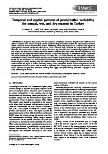
1.2 Study area and gauge data The Tianshan mountains range in the Xinjiang Uygur Autonomous Region of China extends about 1,700 km from east to west and 400 km from north to south. It divides the area in two with north and south having very different natural and geographic landscapes. Unusually, the Tianshan Mountains are high altitude wetlands, and precipitation here regulates water balance and regional environment. Although also affected by the cold, dry air from the Arctic Ocean, the moist air in this region is mainly supplied from the zonal westerly circulation (Wei and Hu 1990). This moist air is forced over the mid Tianshan Mountains, (altitude greater than 3,000 m), giving abundant precipitation. Our study region extended between latitudes 42° and 45°N and longitudes 83° and 88°E that included the mid Tianshan Mountains. The distribution of the stations, regions and DEM (digital elevation model) are shown in Figure 1. The area has seasonal precipitation and a very abrupt orography, with altitudes ranging from 400 to over 5,000 m within 150 km. Precipitation data for 16 stations in this

Figure 1 Terrain of the study area and distribution of the 16 observation stations in this study. The white borders are two typical watersheds and the three rectangles with dash outline are profiles crossed the south - north of mid Tianshan Mountains.

630

J. Mt. Sci. (2012) 9: 628–645

region were collected (Table 1). Five of them are hydrological stations that only have monthly precipitation data between 2000 and 2007 (except Kensiwate). Daily precipitation data for other 11 weather stations were obtained from the Climatic Data Center of the China Meteorological Administration, and were summed to get monthly values. The data have passed rigorous QAQC procedures, with all extreme values being checked and validated. Furthermore, it is well known that snow and/or wind cause errors in rain gauge data (Legates and Willmott 1990); however, in this study we have taken the precipitation data as the actual values. There was no missing data from the monthly precipitation time series for any of the 16 stations; however, because the duration of the precipitation data we collected is not uniform across all stations, we choose to overlap the period between the observed and TRMM 3B43 data.

1.3 DEM data In this study we used the ASTER (Advanced Spaceborne Thermal Emission and Reflection Radiometer) DEM data. This data has a global coverage between 83º N-S latitude with a cell size of 1 arc second (30 m horizontal posting at the Equator). Data used in this study was resampled to 1 km × 1 km resolution. It has been available free

from the NASA WIST since it was released in 2009. DEM data was used to carry out topographic analysis and delineate the major watersheds (see Correction Methodology section).

1.4 Bilinear interpolation method The TRMM 3B43 data can be considered as the representative precipitation value of the 0.25° × 0.25° box. Because the estimation of precipitation by satellites and from observation stations have different spatial and temporal characteristics, it is difficult to match the two datasets well. Instead of using the grid value or the averaging of adjacent grids for a particular point location, bilinear weighted interpolation has been used to calculate the raster value at any point position. Brito et al. (2003) used this method to resample the TRMM 3B43 data for a specific location. In this study we used this method to extract precipitation data at the spatial location of the observed precipitation station from the satellite data. An illustration is shown in Figure 2. In the bilinear interpolation, a simple explanation is followed, i.e. four nearest grid values are used for calculating the value of a particular point (T), and the closer the grid is to the point (Ti), the more influence (weight) it will have. The weights are derived from the spatial locations in a two-

Table 1 Observation stations from which the precipitation data used in this study was taken. Bold represents the five hydrological stations. Station names Bajiahu Baluntai Bayinbuluke Caijiahu Daxigou Manasi Meiyao Shiyanzhan Qingshuihezi Shihezi Shimenzi Wulanwusu Wulumuqi Wusu Xiaoquzi Kensiwate

Elevation (m) 1,302.0 1,738.3 2,458.9 441.0 3,539.0 473.1 1,161.0 1,930.0 1,176.0 443.7 1,886.0 469.3 918.7 478.3 1,871.8 885.0

Latitude (°) 43.950 42.733 43.033 44.200 43.100 44.317 43.900 43.450 43.917 44.316 43.800 44.284 43.783 44.433 43.483 43.950

Longitude (°) 85.417 86.300 84.150 87.533 86.833 86.200 85.850 87.183 86.050 86.050 86.217 85.817 87.617 84.667 87.100 85.417

Precipitation (mm/y) 400.8 210.1 290.2 141.2 453.5 190.9 417.2 450.5 445.0 210.0 495.0 224.7 267.1 169.1 552.1 345.0

Time span 2000.1-2007.12 1958.1-2009.12 1958.1-2009.12 1959.1-2009.12 1959.1-2007.9 1961.1-2007.9 2000.1-2007.12 1978.1-2007.9 2000.1-2007.12 1953.1-2008.12 2000.1-2007.12 1991.1-2007.9 1951.1-2009.12 1957.1-2009.12 1957.1-2007.9 1956.1-2007.12

631

J. Mt. Sci. (2012) 9: 628–645

dimensional space (Gribbon and Bailey 2004). The bilinear interpolation weights can be calculated as follows (Arnold et al. 2002): n

T = ∑ Ti ⋅Wi

(1)

i =1

S Wi = i R

(2)

where n = 4, T is the particular point value, R is the area of the TRMM grid, Wi is the weight. As figure 2 shows, the particular point (T) divides the rectangle surrounding it by the four nearest points into the new four parts; Si is the area of each part.

T2

T3 S2

S3

T

S1

T1

S4

T4

Figure 2 Illustration of bilinear interpolation

This is viewed as a downscaling approach in this study to interpolate the TRMM grid value after correction into a smaller grid (0.01° × 0.01°). This approach could reduce the boundary bias along the border of the 0.25° × 0.25° boxes and generate a continuous surface to allow analysis of the differences of precipitation patterns between the north and south slopes of the Tianshan Mountains (see Results section).

1.5 Correction method Bias-adjustment methods rely either on establishing a relationship between satellite and gauge-based precipitation (where gauge-based measurements are available) or on a combination of several satellite-based estimates in regions with no gauges (Boushaki et al. 2009). In this study, the relationship is derived from regression models for one month periods. The regression analyses were

632

carried out based on observed precipitation data and TRMM 3B43, particularly included location and terrain factors which are the spatial variables for bias correction.

P ′= P ( TRMM ， LCT ， TRR)

(3)

P′ is the estimated value after correction; P(Var1,Var2,…Varn) represents the empirical relationships between observed precipitation data and variables; LCT represents location variables (latitude and longitude) to determine whether there are spatial trends in the performance of the approach; TRR represents terrain variables which are based on local topographic features such as elevation, slope, aspect and roughness. These terrain variables are also commonly used in studies of orographic effects on precipitation (Goodale et al.1998; Katzfey 1994; Bradley et al. 1998; Kurtzman and Kadmon 1999; Wotling et al. 2000; Weisse and Bois 2001). Table 2 summarizes the variables considered in this study. For some variables, the summary value of the topographic feature in a region close to a given point has a greater significance than the value at the point itself (Daly et al. 1994; Wotling et al. 2000). A region the same size as a box in the TRMM grid (0.25° × 0.25°) was generated to extract the terrain features. The box region size matched the spatial resolution of the satellite data, so that the terrain features around the precipitation station would have comparable local scales. To carry out the topographic analysis and generate surfaces of precipitation estimates, GIS was used. For example, values of raster surfaces, such as topographic variables were extracted using zonal statistics and tabulated area functions of the Spatial Analyst Module in ArcGIS (ESRI, Redlands, California). We also used the hydrology analysis function of ArcGIS to delineate the typical river watershed based on the DEM data. The ridgeline of the mid Tianshan south-north slope is also defined. In this study, the flow direction of Manasi river basin is south to north, and the Wulasitai river basin is north to south, and the ridgeline can be clearly seen (shown in Figure 1). To determine which location and terrain variables made significant contributions to the improvement of the precipitation estimates, we used correlation and multiple linear regression analyses. A correlation analysis between the

J. Mt. Sci. (2012) 9: 628–645

Table 2 Description of terrain variables used in this study Variables ID 1 2 3 4 5 6 7 8 9 10 11 12 13 14 15 16 17

Variables Name Elvavg Elvmin Elvmax Elvstd Elvrng Slpavg Slpmin Slpmax Slpstd AspN AspNE AspE AspSE AspS AspSW AspW AspNW

18

Rgh

Description Average elevation in the box region Min elevation in the box region Max elevation in the box region Standard deviation of elevation in the box region Range of elevation in the box region Average slope in the box region Min slope in the box region Max slope in the box region Standard deviation of slope in the box region Proportion of area with north-facing slopes in the box region Proportion of area with northeast-facing slopes in the box region Proportion of area with east-facing slopes in the box region Proportion of area with southeast-facing slopes in the box region Proportion of area with south-facing slopes in the box region Proportion of area with southwest-facing slopes in the box region Proportion of area with west-facing slopes in the box region Proportion of area with northwest-facing slopes in the box region Surface Roughness in the box region: the ratio of curved surface area and projected area

eighteen terrain variables and observed precipitation was performed, and the insignificant variables in that linear relationship were directly excluded from the analysis. Regression analysis was then used to determine the other variables. Regression was carried out stepwise, selecting the variables backwards. In the regression analysis, we first used only the TRMM 3B43 data as the independent variable, then added the location variables (latitude and longitude) into the models, and finally added the terrain variables. While all other variables were selected by a stepwise procedure, only variables that were significant at the 0.05 level were allowed to enter and remain in the models. The advantage for this method is that a variable selected in one step can be eliminated in a later step. In this way, initially all the variables are introduced in a single step and subsequently discarded one by one based on the outset criteria. Each time a variable is removed from the function, the model is recalculated so the variance must be explained globally. This process is continued until a robust regression model between the observed precipitation and the TRMM 3B43 data, station locations and the terrain variables was obtained. The determination coefficient (R2) is considered as a measure of the goodness of fit of the model, and it represents the proportion of the

variation of the dependent variable (monthly precipitation) explained by the regression model. Since the R2 tends to overestimate the goodness of fit of the model, we also calculated an adjusted R2, which compensates for the optimistic trait in the determination coefficient. Unlike R2, the adjusted determination coefficient does not necessarily increase when additional variables are added to an equation. The reliability of the corrected TRMM 3B43 estimates was evaluated using the RMSE (rootmean-square error), which is frequently used as a measure of the differences between values predicted by a model and those actually observed. This error is absolute and maintains the unit of measurement, and represents that of the best estimation parameters. We also validated these correction factors based on a comparison with the observed monthly precipitation data for each station, especially the Kensiwate station, which was not used in the regression models. The aim was to show the improvement in the estimation of precipitation. n

RMSE =

∑ (T − O ) i =1

i

2

i

n

(4)

633

J. Mt. Sci. (2012) 9: 628–645

n

R2 =

∑ (T

− O )2

∑ (O

−O)

i =1 n

i =1

i

i

(5)

Ra2 = 1 −（1 − R 2）⋅

2

n −1 n − k −1

(6)

Ti is the TRMM 3B43 estimation after correction, Oi is the observed precipitation value, O is the mean of the observed data, k is the total number of variables, n is the sample size. We extracted the necessary terrain variables for each TRMM 3B43 data grid in our study area, and then calculated the estimation precipitation value using the best regression models. However, due to the low resolution (0.25° × 0.25°), the corrected precipitation value changed in a nonuniform step manner, and was inconsistent with the scale of our study.We interpolated the grid to a small (0.01° × 0.01°) grid using the bilinear interpolation method introduced above. Once this was done, spatial variation analysis of precipitation was carried out. We selected three profiles that were perpendicular to the ridgeline of mid Tianshan Mountains to analyze the vertical distribution differences of precipitation between the north and south slopes. We also chose one typical river basin for both of the north and south slopes of the Tianshan Mountains to analyze the characteristics of the precipitation on a basin scale. For the purposes of the comparison, we chose the Manasi river basin (north slope) and Wulasitai river basin (south slope) because they have comparable features, i.e. similar basin areas and flows (Figure 1).

2

small proportion of annual precipitation. For the summer months, the range of the bias between satellite estimates and observed data is large (e.g. +64 to -139 mm in July), a quite different spatial pattern to that of the winter. The spatial distribution of the mean absolute relative biases between the TRMM 3B43 and observed data over all years of the study period is shown in Figure 4. It generally shows that TRMM 3B43 data tended to underestimate precipitation consistently in mountainous regions, especially on the north slopes. For example, the annual precipitation is almost 50% underestimated at the Xiaoquzi station. We also calculated the correlation coefficients between the observed and TRMM 3B43 estimated values for each station over all months. As Figure 5 shows, the performance of TRMM 3B43 estimates appeared to have strong correlations to the observed precipitation values in the mountainous regions, but was only weakly correlated in the low elevation areas. Overall, we can conclude that the TRMM 3B43 data has strong correlation and large bias with the observed data in mountain area, and they must be corrected before being used. We found that the performance of TRMM 3B43 data in south slope situations is different from that in the north. The estimation bias is low

Results

2.1 Performance of the TRMM 3B43 data Figure 3 shows the difference of monthly precipitation between observed and TRMM 3B43 data averaged for all the months of the study period with all stations pooled together. In general, TRMM 3B43 underestimated the station precipitation except for a small winter overestimation for January, February, and December. The overestimation was a relatively

634

Figure 3 Box plot of the monthly variations of the deviation between the TRMM 3B43 and observed data for all station. The box plot summarizes five numbers: the minimum, the maximum, the lower quartile, the median, the upper quartile. There are 159 data samples for January to September respectively and 154 samples for October to December respectively used in the calculation. In general, the TRMM 3B43 data underestimated the observed data during the wet period.

J. Mt. Sci. (2012) 9: 628–645

Figure 4 Spatial distribution of the mean absolute relative biases between TRMM 3B43 and observed data averaged for all the year during study period (TRMM 3B43 precipitation estimates as ratios to the station observations).

Figure 5 Correlation coefficients between TRMM 3B43 and observed data at each station. (At the 0.01 level)

and the estimates are in very good correlation with the observed precipitation at the two south slope stations. It seems the TRMM 3B43 monthly precipitation has a high accuracy on the southern slopes of the Tianshan Mountains. However, due to the modest number of stations, this conclusion remains uncertain.

2.2 Correction of the TRMM 3B43 data We extracted 18 potential terrain variables that could affect precipitation distribution in the study area (Table 2). To select those variables that can make statistically significant contributions to predicting the spatial pattern of precipitation, we

635

J. Mt. Sci. (2012) 9: 628–645

conducted correlation analysis using station precipitation data for each month against the topographic variables. Fifteen terrain variables had statistically significant correlation coefficients (at the 0.05 level) with the station precipitation for at least 1 month when all data in the study period were pooled together. Three variables that did not have any significant correlation coefficients were Elvrng and Aspsw, Aspw; these were excluded from the subsequent regression analysis. Table 3 shows the result of stepwise regression on observed data. With each step, the R2 values or explained variances improved. For stepwise regression using location variables, latitude entered all models except for May, but longitude was only included for May, June, July, August (Table 3a). These results appear to show that longitude mainly influences the precipitation distribution in summer months, when the weather is rainy and a westerly circulation prevails. On average, the adjusted R2 values increased from 0.4375 when using TRMM 3B43 alone, to 0.4766 when location variables were added, and to 0.6302 when the terrain was added to the models (Table 3). For comparison, the reported correlations between satellite estimates and gauge observations in several studies would be equivalent to R2 values of 0.3 to 0.6 in most cases (Yin et al. 2008; Adler et al. 2001; Sealy et al. 2003).

It is noteworthy that the performance of the models in the cold season is not as good as that in the warm seasons. Possibly this is because the original satellite estimates, which perform worse in the cold season, have the dominant influence. However, the final models represent a significant improvement compared with only the TRMM 3B43 data. Table 4 represents the variables and regression coefficients of the final models to illustrate how terrain variables can be used as correction factors with different monthly weights to improve TRMM 3B43 precipitation estimates. Four variables (Elvstd, Slpmin, Slpmax and Slpstd ) that were not significant (P = 0.05 ) were excluded in the process of regression analysis. Hence, only 11 terrain variables retained in the final model. We plotted the monthly precipitation of the TRMM 3B43 estimates, and the model-estimated values against the station observed values in Figure 6. The improvement over the original TRMM3B43 estimates is obvious. The corrected precipitation estimates explained over 81% of the variance in the observed precipitation as compared to 64% by TRMM3B43 alone, and the RMSE decreased 34% after correction. The fit of the lines clearly show that the TRMM3B43 data generally underestimated precipitation and became very close to observed data after correction.

Table 3 Results of regression analysis are based on all study period data pooled together for each month. (a). R2 of regression models: observed precipitation VS TRMM 3B43 Jan.

Feb.

Mar.

Apr.

May

Jun.

Jul.

Aug.

Sep.

Oct.

Nov.

Dec.

R²

0.26

0.57

0.30

0.23

0.40

0.59

0.50

0.59

0.42

0.34

0.49

0.44

Adjusted R²

0.25

0.57

0.29

0.23

0.39

0.59

0.49

0.58

0.41

0.34

0.48

0.44

(b). R2 of regression models: observed precipitation VS TRMM 3B43 (forced) and location variables (stepwise) Jan.

Feb.

Mar.

Apr.

May

Jun.

Jul.

Aug.

Sep.

Oct.

Nov.

Dec.

R²

0.32

0.58

0.32

0.25

0.40

0.67

0.68

0.72

0.43

0.40

0.54

0.50

Adjusted R²

0.31

0.57

0.31

0.24

0.40

0.66

0.67

0.71

0.42

0.39

0.53

0.50

Variables entered

Lat

Lat

Lat

Lat

Lat

Lat

Lat

Lat

Lat

Lat

Lat

Lon

Lon

Lon

Lon

(c). R2 of regression models: station precipitation VS TRMM 3B43 (forced), location, and terrain variables (stepwise). The entered variables are shown in Table 4 Jan.

Feb.

Mar.

Apr.

May

Jun.

Jul.

Aug.

Sep.

Oct.

Nov.

Dec.

R²

0.48

0.68

0.57

0.68

0.70

0.76

0.71

0.77

0.63

0.60

0.64

0.62

Adjusted R²

0.44

0.66

0.54

0.66

0.69

0.74

0.70

0.76

0.61

0.58

0.61

0.60

636

J. Mt. Sci. (2012) 9: 628–645

Table 4 Regression models to predict station precipitation using satellite estimates, geographic location, and terrain variables. All independent variables in the models are statistically significant at the 0.05 level except the blanks, which represent the variables not entered the model. Var. TRMM

Jan.

Feb.

Mar.

Apr.

Regression coefficients May Jun. Jul. Aug.

Sep.

Oct.

Nov.

Dec.

0.487

0.900

0.852

0.847

1.1566

0.856

0.933

1.043

0.782

0.641

-2.583

-9.755

-8.481

3.369

3.305

-4.917

-3.023

-3.571

-2.909

-70.725

-31.919

-76.367

-58.119

-34.720

-36.308

-28.346

0.039

0.096

-0.024

-0.020

-0.045

-0.084

Lon Lat

-11.810

-25.003

-68.626

Eleavg Elemin

-0.073

-0.036

0.062

0.074

0.023

-0.099

Elemax

-0.006

Slpavg

15.109

-0.039

0.925

0.815

0.027

-0.028

-0.015

-0.021 4.475

-16.669

15.1685

558.673

146.971

531.106 -65.055

Rgh

-278.675

Aspe

-152.323

-79.456

-174.214

Aspn

-125.808

-35.448

-95.897

Aspne

-122.006

-54.333

-56.765

-170.975

Aspnw

-155.623

-71.039

-152.267

-256.325

Asps

-366.741

-198.295

-169.510

-560.656

Aspse Con.

-156.788

-91.499

966.699

1398.324

3383.577

3891.460

2.010 97.558 136.465 129.063

-40.354

3.497

-156.506

-87.945 -316.131 253.004

543.218

1049.106

3318.294

-296.045

116.424

156.373

-77.623

-100.598

-43.067

-83.979

-79.793

-84.137

-105.124

-154.297

-123.431

-161.427

-247.313

-251.103

-260.677

-24.224

-140.015

-71.33

1913.412

1364.218

151.504

48.616

203.987

-62.958

3.131

2970.175

1881.809

Note: Var. = Variables; Con. = Constant

Figure 7 Mean monthly precipitation of TRMM3B43 and corrected estimations compared to the observed at Kensiwate station. It shows obvious improvement in April and May, and a more reasonable distribution during the year.

Figure 6 TRMM 3B43, and model estimates plotted against the observed monthly precipitation values at all stations. The dash line indicated fit line of the original TRMM3b43 and observed data, and the solid is after corrected.

The R² and RMSE were also calculated at each station to illustrate the effects of correction (Table 5). It shows that the R²of corrected and observed data ranged from 0.7 to 0.96 at mountain stations, and the RMSE decreased to an average of 14. The R2 did not improve very much at Baluntai and Bayinbuluke stations on the south slope.

Nevertheless, it does explain over 90% of the variance in the observed precipitation, and the RMSE was smaller. The Kensiwate station, which did not participate in the regression models, showed an improvement in its R2 value of 33.85%, and a drop in the RMSE of 23.71%. Additionally, according to Figure 7, the mean of monthly corrected precipitation was very close to the observed data at this station especially in April and May, and the distribution during the year is more reasonable. Compared with the original TRMM 3B43 data, the corrected estimations were also significantly improved on an annual time scale (Figure 8).

637

J. Mt. Sci. (2012) 9: 628–645

Table 5 R² and RMSE of the TRMM 3B43, and model estimates compare to the observed monthly precipitation values at each station. (Bold represent the station in mountain area and the Italic indicate the station did not participate in the regression analysis) Station Name Bajiahu Bayinbuluke Baluntai Caijiahu Daxigou Manasi Meiyao Qingshuihezi Shihezi Shimenzi Shiyanzhan Wulanwusu Wulumuqi Wusu Xiaoquzi Kensiwate

Original TRMM 3B43 R² RMSE 0.63 21.36 0.88 11.68 0.96 8.51 0.52 10.52 0.75 29.04 0.29 15.34 0.55 22.36 0.57 23.84 0.36 14.02 0.68 25.35 0.67 29.58 0.341 14.92 0.81 12.34 0.25 13.19 0.71 38.07 0.53 19.50

Corrected estimates R² RMSE 0.75 17.03 0.915 8.94 0.965 6.09 0.515 8.59 0.88 17.67 0.38 12.99 0.70 16.01 0.73 16.14 0.55 10.50 0.82 15.37 0.81 18.04 0.56 10.71 0.85 9.30 0.42 10.90 0.83 18.99 0.71 15.27

also provides the possibility of understanding the spatial variability of precipitation that exists in the mid Tianshan Mountains.

2.3 Spatial pattern of precipitation over the middle Tianshan Mountains

Figure 8 Annual precipitation of TRMM3B43 and corrected estimations compared to the observed at each station (averaged from all study periods).

These results suggest that terrain and location variables can further improve the 3B43 data for all months by using the regression models. It is impossible to eliminate the bias completely，but our results show that the bias can be significantly reduced and the corrections have reasonable annual distribution. In general, the corrected estimations were very close to the observed data at all stations in the study area. The corrected data

638

All the TRMM 3B43 monthly precipitation grids during 1998-2009 in our study area were corrected using the best regression models, and then the estimated precipitation values were interpolated to a small grid (0.01° × 0.01°) by the bilinear interpolation method. Figure 9 represents the spatial distribution of annual average precipitation in the mid Tianshan Mountains. It shows that the spatial variations of precipitation are more complex in mountainous areas than on the plains. The precipitation increases slightly with elevation in the low mountain area of the northern slopes, and shows irregular zonation of high precipitation in the medium-high mountain area. Although the precipitation amount changes from area to area, it can be clearly seen that precipitation over the mountains is much higher than that over the plain. According to Figure 9, the maximum precipitation reached about 600-800 mm on the northern slopes of the mid Tianshan Mountains. In sharp contrast,

J. Mt. Sci. (2012) 9: 628–645

Figure 9 Spatial distribution of 12-yr averaged (1998-2009) annual precipitation over the mid Tianshan Mountains.

Figure 10 Profiles of topography and precipitation. The black lines and dark gray shading show the mean elevation (m) and range of elevations along the profiles indicated in Figure 1. The dashed line is the 12yr average annual precipitation (mm/yr) estimated with the corrected TRMM3B43 precipitation data. Light gray shading indicates the range of precipitation values.

a low precipitation center exists in the Small Youerdus Basin which has only about 150 mm annual precipitation. It indicates that the mountains influence the amount of precipitation and the importance of the mountain range on the spatial distribution of precipitation is highlighted by the confinement of the precipitation maxima to the northern slopes. To further analyze the differences in

precipitation distribution between northern and southern slope, we selected three topographic profiles which cross the ridgeline of the mountains (The ridgeline was defined by the two typical watersheds in this study, shown in Figure 1). Figure 10 shows the relationship between precipitation and topography on the three profiles. The Small Youerdus Basin on the southern slope is a low precipitation region that was clearly shown again

639

J. Mt. Sci. (2012) 9: 628–645

Figure 11 Correlation of annual average precipitation and elevation in basins.

on profile A and B. In comparison with profiles A and B, the correlation of precipitation and topography is simple on profile C, but still quite different between the two sides of the mountains. It shows that precipitation on northern slopes is always greater than on the southern slopes at the same altitude; as there is a high mountain peak, the precipitation on the leeward slope declined slightly (Note that the highest peak in these profiles is not necessarily on the ridgeline we defined). Precipitation decreases with increasing elevation at a certain altitude on the northern slopes on all three profiles. In other words, Figure 10 shows that the distribution of precipitation does not always increase monotonically with elevation. The spatial variation of precipitation was analyzed on the basin scale. Two typical river basins (Manasi River and Wulasitai River) were divided into several elevation bands with a range of about 200 m. The average elevation and annual precipitation in each band were calculated. Although this leads to a homogenization of the different elevations in each band, the results still reflect the general trend. As Figure 11 shows, there were significant differences in vertical distribution of precipitation between the two watersheds. In the Manasi river basin, the vertical increase in the rate of annual precipitation is 143.05 mm/km (below about 2,500 m); between about 2,500 m and 3,700 m the precipitation decreased with altitude (81.81mm/km), and then increased again(65.7 mm/km) above 3,700 m (Table 6). This is probably due to the orographic precipitation effect of the high mountains, so that the incoming moist

640

Table 6 Increasing rate of precipitation in different elevation range of two typical river basins. (The correlations were all significant at the 0.01 level) BN

Manasi River

Wulasitai River

ER 1,0002,500 2,5003,700 3,7005,000 1,4003,200 3,2004,200

IR

CC

143.05

0.9715

-81.01

0.9947

65.7

0.9415

76.57

0.9836

268.64

0.9852

BP

545.38

323.65

Note: BN = Basin Name; ER = Elevation Range (m); IR = Increasing Rate (mm/km); CC = Correlation Coefficient; BP = Basin Precipitation (mm)

northwesterly air is denuded of the bulk of its water and hence delivers very little rainfall to the southern slope. In sharp contrast, precipitation increased monotonically with elevation in the Wulasitai river basin, showing a moderate increase below 3,200 m, a dramatic increase (about 268 mm/km) above 3,200 m. The rain shadow mechanism above also explains the annual average precipitation to the Manasi River basin. The spatial patterns also changed with season in the mid Tianshan Mountains (Figure 12). Although precipitation in summer (June, July and August) accounts for more than half of yearly amount in both watersheds, it shows different morphology. In the area below the elevation of 2,500 m in the Manasi River basin, April to August are the main precipitation months of the year, and compared to the high altitude region, the

J. Mt. Sci. (2012) 9: 628–645

Figure 12 Variations of monthly precipitation in watersheds at different elevations

precipitation changes are moderate in these months. Seasonal variation of precipitation in all elevation bands of the Wulasitai river basin is similar to that in high mountain area of Manasi river basin, i.e. the precipitation changes significantly from month to month. July has the highest precipitation, and had the highest rainfall in the highest band of both watersheds. Figure 12 also shows a remarkable phenomenon: the precipitation in the high attitude area is less than the low area in the Manasi River basin in cold seasons.

3

Discussion

mountainous regions are usually in solid form (snowfall). At present, remote sensing of snowfall is still a difficult process, as snowflakes (or frozen precipitation) have different sizes, shapes, and densities resulting in complex radar echoes (Bookhagen and Burbank 2010).The only input into the combined TRMM 3B43 product for snow comes from the AMSU-B precipitation data: first regions of falling snow over land is identified through the use of AMSU-A measurements at 53.8 GHz, and then falling snow is assigned a rate of 0.1 mm/hr（Huffman and Bolvin 2012). The simple assigned snowfall rate may be the reason resulting in underestimating precipitation for high mountainous area.

3.1 The uncertainty of the TRMM 3B43 precipitation estimates

3.2 The orographic effect of topographic features on precipitation

Although TRMM 3B43 data has many advantages, it also has some uncertainty. There are sampling and instrumental errors, and inevitable random error caused by different kinds of sensor. These errors affect the accuracy of the precipitation product. Also for using these data, Barros et al. (2006) found that the TRMM PR had difficulties in detecting precipitation at high elevations. And many studies showed that these data sets are often underestimated for mountainous regions (Berg et al. 2006; Huffman et al. 2007; Barros et al. 2004; Anders et al. 2006). In this study, we also found the TRMM 3B43 product underestimated the precipitation in mid Tianshan Mountains. This is probably due to precipitation occurred in the high

The orographic effect of topographic features on precipitation has a well-documented and significant influence on precipitation patterns. For example, Smith (1979) found that topography itself has a profound effect on spatial patterns of precipitation both globally and regionally. It is well known that mountains influence the flow of air and disturb the vertical stratification of the atmosphere by acting as physical barriers and as heat sources or sinks (Barros and Lettenmaier 1994). Roe et al. (2003) described the mechanisms of orographic precipitation, including forced ascent on windward slopes and adiabatic warming on the leeward slopes when mountain ranges lie across the prevailing moisture-laden wind flows. These

641

J. Mt. Sci. (2012) 9: 628–645

mechanisms depend on both topography and the conditions of the air parcel upwind of the mountains (Anders et al. 2006). The temperature, moisture content, and velocity of the incoming air, as well as the topographic characteristics, work together to determine how the atmosphere interacts with the mountains (Houze 1993). This work has not explained the spatial variation of precipitation in detail based on the mechanisms of the physical processes of the multiple factors determined, for the reason that limitations of the spatial and temporal resolution of the datasets. However, we have shown that topographic variables, which are easily extracted from the DEM, contributed significantly in the correction of the biases in satellite rainfall estimates (Table 4). Additionally, this approach still allows understanding of the effect of topographic structure on the spatial pattern of precipitation in the mid Tianshan Mountains, to some extent still based on a statistical approach. Many studies in the Himalayas have indicated that the pattern of precipitation is strongly controlled by the topography, and there is a dramatic reduction of precipitation in the rain shadow north of the Himalayas (Barros et al. 2004; Bodo and Douglas 2006; Anders et al. 2006). Similarly, we have concluded that topographic features dominate the significant differences of spatial distribution of precipitation in the mid Tianshan Mountains. Wei and Hu (1990) found that the relative humidity on the northern slopes is 40% higher than that of the southern. It can be interpreted as south being in the rain shadow of the north. Therefore, there is a significant difference in the spatial pattern of precipitation between the north and south slopes of the mid Tianshan Mountains.

3.3 Special features of precipitation distribution in the mid Tianshan Mountains Based on our limited data, we were unsure about the reasons for the formation of second maximum precipitation zone in the northern slope of the mid Tianshan Mountains, according to other studies (Fu 1992; Chen et al. 1980; Wei and Hu 1990; Shen and Liang 2004), it seems likely that the strong evaporation of permanent snow and

642

glaciers (above about 3,700 m), allows the humidity to increase, making it possible to form abundant precipitation. In cold seasons, the precipitation in the high attitude area is less than the low area in the Manasi River basin in northern slope. A reasonable explanation is that this is caused by a temperature inversion that occurred over the northern slopes of the mid Tianshan Mountains (Han et al. 2002; Aizen et al. 1996). This variation of precipitation returned to normal when the temperature inversion ended. This phenomenon was not observed in the Wulasitai river basin on the southern slopes of the Tianshan Mountains. Similar seasonal gradients have been observed before (Han et al. 2004). Additionally, the lack of sufficient and well distributed sites on the southern slopes of the Tianshan Mountains means that there may be some uncertainty about the estimations of precipitation in this area when building the regression models. However, the good performance of the original TRMM 3B43 data on the southern slopes (Table 5) and consistency with the results from a previous study (Han et al. 2004) increases our confidence in our results.

4

Conclusions

In this study, we first analyzed the biases of TRMM 3B43 monthly precipitation estimates over the mid Tianshan Mountains. The biases of the TRMM 3B43 data have different regional patterns, and largely underestimate the precipitation for most parts of the study region, especially in the high altitude mountain area on the northern slopes. The spatial patterns of the biases varied monthly, suggesting seasonal patterns of the influencing factors. In order to select the variables that can be used as correction factors to improve TRMM3B43 precipitation estimates over the study area, we extracted terrain variables around the stations. After a preliminary correlation analysis, 15 terrain variables were included in stepwise regression analysis. By adding the topographic variables to the regression models, the performance of the satellite estimates can be improved significantly. These results suggest that it is feasible to use these terrain

J. Mt. Sci. (2012) 9: 628–645

and location variables to improve satellite estimates. We recalculated all the TRMM 3B43 monthly precipitation grids between 1998 and 2009 in our study area using the best regression models. On this basis, variation patterns of precipitation in the mid Tianshan Mountains show that there is more precipitation on the northern than the southern slopes. Clearly, the mountains have a strong effect on the amount and spatial distribution of precipitation in the area. This is underscored by the confinement of the precipitation maxima to the northern slope. To a great extent the results are well explained by a general understanding of and the orographic effects of the mountains. The annual amount of precipitation on windward (northern slope) is always greater than that on the leeward (southern slope) at the same attitude. The precipitation on the leeward slope changes slightly with elevation. The correlations of topography with precipitation indicate the importance of the mountain range in providing the moisture for the precipitation events. A negative increasing rate of annual precipitation in the vertical direction exists on the northern slope shows that annual precipitation does not always increase monotonically with the elevation. Basin scale analysis of the spatial variations of precipitation showed there were significant differences in the vertical distribution of precipitation. That is mainly affected by topography. The spatial distribution of precipitation also shows different seasonal patterns in different regions. It is quite unique that the precipitation in the higher attitude area is less than that over the lower area on the northern slopes in

cold seasons. The large gradients in seasonal precipitation found in this work are not simply related to elevation. It supports the view the distribution of precipitation may also be affected by some seasonal variables, such as sources of moist air, wind direction and temperature. Finally, it should be noted that our approach in correcting the TRMM 3B43 data is entirely empirical and limited by the spatial and temporal resolution. Although we cannot identify the specific physical mechanisms of the orographic effect, the correction much improved the prediction, and we can explain the external features of the spatial pattern over the mid Tianshan Mountains. However, much work remains to be done in this data-scarce mountain region. Measuring and modeling spatial variability of precipitation in mountainous areas will no doubt provide new and interesting insights into the interrelationships among climate, hydrology and topography.

Acknowledgments The TRMM3B43 data were provided by the NASA/Goddard Space Flight Center's Mesoscale Atmospheric Processes Laboratory and PPS. We thank the Climate Data Center at the National Meteorological Information Center of the China Meteorological Administration for providing the station precipitation data used in this study. This study is supported by the 973 Program of China (Grant No. 2010CB951002), Natural Science Foundation of China (Grant No. 41130641). We thank the three referees for the very good comments.

References Adler RF, Huffman GJ, Chang A, et al. (2003) The version-2 global precipitation climatology project (GPCP) monthly precipitation analysis (1979-present). Journal of Hydrometeorology 4: 1147-1167. Adler RF, Kidd C, Petty G, et al. (2001) Intercomparison of global precipitation products: The third precipitation intercomparison project (PIP-3). Bulletin of the American Meteorological Society 82: 1377-1396. AghaKouchak A, Nasrollahi N, Habib E (2009) Accounting for uncertainties of the TRMM satellite estimates. Remote Sensing 13: 606-619. AizenVB, Aizen EM, Melack JM (1996) Precipitation, melt and runoff in the northern Tien Shan. Journal of

Hydrometeorology 186: 229-251. Almazroui M (2011) Calibration of TRMM rainfall climatology over Saudi Arabia during 1998-2009. Atmospheric Research 99: 400-414. Anders AM, Roe GH, Hallet B, et al. (2006) Spatial patterns of precipitation and topography in the Himalaya. Geological Society of America Special Paper 398, Geological Society of America. pp 39-53. Anderson NF, Cedric AG, Jeffrey LS (2005) Characteristics of Strong Updrafts in Precipitation Systems over the Central Tropical Pacific Ocean and in the Amazon. Journal of Applied Meteorology and Climatology 44: 731-738. Aragao LEOC, Malhi Y, Cuesta RMR, et al. (2007) Spatial

643

J. Mt. Sci. (2012) 9: 628–645

patterns and fire response of recent Amazonian droughts. Geophysical Research Letters 34: L07701. Arnold DN, Boffi D, Falk RS (2002) Approximation by quadrilateral finite element. Mathematics of Computation 71: 909-922. Barros AP, Chiao S, Lang TJ, et al. (2006) From weather to climate—seasonal and interannual variability of storms and implications for erosion process in the Himalaya. Geological Society of America Spatial Paper 398. Penrose Conference Series. pp 17-38. Barros AP, Kim G, Williams E, et al. (2004) Probing orographic controls in the Himalayas during the monsoon using satellite imagery. Natural Hazards and Earth System Sciences 4: 29-51. Barros AP, Lettenmaier DP (1994) Dynamic modeling of orographically induced precipitation. Review of Geophysics 32: 265-284. Bell TL, Abdullah A, Martin RL, et al. (1990) Sampling errors for satellite-derived tropical rainfall: Monte Carlo study using a space–time stochastic model. Journal of Geophysical Research 95(D3): 2195-2205. Beniston M, Diaz HF, Bradley R S (1997) Climatic change at high elevation sites an overview. Climatic Change 36: 233-251. Berg W, Ecuyer T, Kummerow C (2006) Rainfall climate regimes: the relationship of regional TRMM rainfall biases to the environment. Journal of Applied Meteorology and Climatology 45: 434-453. Bodo B, Douglas WB (2006) Topography, relief, and TRMMderived rainfall variations along the Himalaya. Geophysical Research Letters 33: L08405. Bookhagen B, Burbank DW (2010) Toward a complete Himalayan hydrologic budget: Spatiotemporal distribution of snowmelt and rainfall and their impact on river discharge. Journal of Geophysical Research 115: F03019. Boushaki FI, KL Hsu, Sorooshian S, et al. (2009) Bias adjustment of satellite precipitation estimation using groundbased measurement: A case study evaluation over the southwestern United States. Journal of Hydrometeorology 10: 231-1242. Bradley SG, Dirks KN, Stow CD (1998) High resolution studies of rainfall on Norfolk Island, Part III: a model for rainfall redistribution. Journal of Hydrometeorology 208: 194-203. Brito AE, Chan SH, Cabrera SD (2003) SAR image super resolution via 2-D adaptive extrapolation. Multidimensional Systems and Signal Processing 14: 83-104. Chen WL, Weng DM, QianLQ, et al. (1980) Discussions about calculation method of temperature and precipitation in mesoscale mountain area. Journal of Nanjing Institute of Meteorology 1: 95-104. Collischonn B, Collischonn W, MorelliC (2008) Daily hydrological modeling in the Amazon basin using TRMM rainfall estimates. Journal of Hydrology 360(1-4): 207-216. Condom TRP, Espinoza JC (2011) Correction of TRMM 3B43 monthly precipitation data over the mountainous areas of Peru during the period 1998–2007. Hydrological Processes 25(12): 1924-1933. Daly C, Neilson RP, Phillips DL (1994) A statistical topographic model for mapping climatologically precipitation over mountainous terrain. Journal of Applied Meteorology33: 140158. Dingman SL (2002) Physical hydrology: Upper Saddle River, New Jersey, Prentice Hall. pp 646. Franchito SH, Brahmananda R, Vasques AC, et al. (2009) Validation of TRMM PR Monthly rainfall over Brazil. Journal of Geophysical Research 114: D02105. Fu BP (1992) The impaction of topography and elevation on precipitation distribution. Acta Geographical Sinica 4: 302314. (In Chinese) Gao ZY, Zang JX, Liao FJ, et al. (2003) Change of Summer Precipitation during 40 years Period at North Slope of Middle Tiansan Mountains of Xinjiang. Journal of Desert Research 23(5): 581-585. (In Chinese) Gebremichael M, Anagnostou EN, BitewMM (2010) Critical

644

Steps for Continuing Advancement of Satellite Rainfall Applications for Surface Hydrology in the Nile River Basin. JAWRA Journal of the American Water Resources Association 46: 361-366. GoodaleCL, Alber JD, OllingerSV (1998) Mapping monthly precipitation, temperature and solar radiation for Ireland with polynomial regression and digital elevation model. Climate Research 10: 35-49. Grecu M, AnagnostouEN (2001) Overland precipitation estimation from TRMM passive microwave observations. Journal of Applied Meteorology 40: 367-1380. Gribbon KT, Bailey DG (2004) A novel approach to real time bilinear interpolation. In: Proceedings of the Second IEEE International Workshop on Electronic Design, Test and Applications. pp 126. Groisman PV, Legates DR (1994) The accuracy of United States precipitation data, Bulletin of the American Meteorological Society 75: 215-227. Han TD, Ye BH , Jiao KQ (2002) Temperature variations in the southern and northern slopes of Mt. Tianger in the Tianshan Mountains. Journal of Glaciology and Geocryology 24(5): 567-570. (In Chinese) Han TD，Ding YJ，Ye BS, et al. (2004) Precipitation Variations on the Southern and Northern Slopes of the Tianger Range in Tianshan Mountains. Journal of Glaciology and Geocryology 6: 761-766. (In Chinese) Houze RA (1993) Cloud dynamics. Academic Press, Boston. p 573. Huffman GJ, Adler R F, Arkin P, et al. (1997) The Global Precipitation Climatology multi satellite Project (GPCP) combined precipitation dataset. Bulletin of the American Meteorological Society 78: 5-20. Huffman GJ, Adler RF, Bolvin DT, et al. (2007) The TRMM multi-satellite precipitation analysis: quasi-global, multi-year, combined-sensor precipitation estimates at fine scale. Journal of Hydrometeorology 8(1): 38-55. Huffman GJ, Adler RF, Rudolph B, et al. (1995) Global precipitation estimates based on a technique for combining satellite based estimates, rain gauge analysis, and NWP model precipitation information. Journal of Climate 8: 1284-1295. Huffman GJ, Bolvin DT (2012) TRMM and other data precipitation data set documentation. Laboratory for Atmospheres, NASA Goddard Space Flight Center and Science Systems and Applications, pp 25. [Available online at ftp://precip.gsfc.nasa.gov/pub/trmmdocs/3B42_3B43_doc.p df] Immerzeel WW, van Beek LPH, Bierkens MFP (2010) Climate change will affect the Asian water towers. Science 328: 1382– 1385. KatzfeyJJ (1994) Simulation of extreme New Zealand precipitation events. Part I: sensitivity to orography and resolution. Monthly Weather Rev 123(3): 737-754. Kurtzman D, Kadmon R (1999) Mapping of temperature variables in Israel: a comparison of different interpolation methods, Climate Research 13: 33-43. Legates DR, Willmott CJ (1990) Mean seasonal and spatial variability in gauge-corrected, global precipitation. International Journal of Climate 10: 111-127. Li X, Ren YY, Tan GH, et al. (2005) Precipitation over the Middle Tianshan Mountains and Their Northern Slopes: Variations and Their Cause. Journal of Glaciology and Geocryology 27(3): 381-388. (In Chinese) Muhammad JMC, Wim GMB (2011) Local calibration of remotely sensed rainfall from the TRMM satellite for different periods and spatial scales in the Indus Basin, International Journal of Remote Sensing 8(33): 2603-2627. Nesbitt SW, Zipser EJ (2003) The diurnal cycle of rainfall and convective intensity according to three years of TRMM measurements. Journal of Climate 16: 1456-1475. North G, NakamotoS (1989) Formalism for comparing rain estimation designs. Journal of Atmospheric and Oceanic Technology 6: 985-992.

J. Mt. Sci. (2012) 9: 628–645

Roe GH, Montgomery DR, HalletB (2003) Orographic precipitation and the relief of mountain ranges. Journal of Geophysical Research 108(2315). p 12. Sealy A, Jenkins GS, Walford SC (2003) Seasonal/ regional comparisons of rain rates and rain characteristics in West Africa using TRMM observations. Journal of Geophysical Research 108(4306). p 21. Shen YP, Liang H (2004) High Precipitation in Glacial Region of High Mountains in High Asia: Possible Cause. Journal of Glaciology and Geocryology 24(6): 806-809. (In Chinese) Shin KS, North GR (1988) Sampling error study for rainfall estimate by satellite using a stochastic model. Journal of Applied Meteorology and Climatology 27: 1218-1231. Sinclair MR, Wratt DS, Henderson RD, Gray WR (1997) Factors affecting the distribution and spillover of precipitation in the Southern Alps of New Zealand—A case study: Journal of Applied Meteorology 36: 428-442. Smith RB (1979) The influence of mountains on the atmosphere. Advances in Geophysics 21:87-230 Tian YD, Christa D. Peters-Lidard, John B. Eylander (2010) Real-Time Bias Reduction for Satellite-Based Precipitation Estimates. Journal of Hydrometeorology, 11: 1275-1285. Tobin KJ, Marvin EB (2010) Adjusting Satellite Precipitation Data to Facilitate Hydrologic Modeling. Journal of Hydrometeorology 11: 966-978. Wei WS, Hu RJ (1990) Precipitation and climate conditions in

Tianshan Mountains. Arid Land Geography 13(1): 29-36. (In Chinese) Weisse AK, Bois P (2001) Topographic effects on statistical characteristics of heavy rainfall and mapping in the French Alps. Journal of Applied Meteorology 40 (4): 720-740. Wentz F J (1991) User’s manual SSM/I antenna temperature tapes, revision1. Remote Sensing System (RSS) Technology Report 120191. p 70. Wilk J, Kniveton D, Andersson L, et al. (2006) Estimating rainfall and water balance over the Okavango River Basin for hydrological applications. Journal of Hydrology 331: 18-29. Wotling G, Bouvier C, Danloux J, Fritsch J M (2000) Regionalization of extreme precipitation distribution using the principal components of the topographical environment. Journal of Hydrology 233: 86-101. Yan J, Gebremichael M (2009) Estimating actual rainfall from satellite rainfall products. Atmospheric Research 92: 481-488. Yin ZY, Liu X, Zhang X, et al. (2004) Using a geographic information system to improve special sensor microwave imager (SSM/I) precipitation estimates over the Tibetan Plateau. Journal of Geophysical Research 109: D03110. Yin ZY, Zhang XQ, Liu XD, et al. (2008) An assessment of the biases of satellite rainfall estimates over the Tibetan plateau and correction methods based on topographic analysis. Journal of Hydrometeorology 9(3): 301-326.

645