invalidate a two-vector test for a network break just as charge sharing can. Furthermore, ... approach needs to use the worst case capacitance value.
Charge-Based Fault Simulation for CMOS Network Breaks Haluk Konuk
F. Joel Ferguson
Tracy Larrabee
Abstract We de ne a network break as a break fault in the p-network or in the n-network of a CMOS cell that breaks one or more transistor paths between the cell output and Vdd or GND. Previous work, mostly in the context of transistor stuck-open faults, studied test invalidation due to transient paths to Vdd or GND, and due to charge sharing. In this paper we show the importance of Miller feedthrough and feedback capacitances in network break test invalidation, which was ignored by previous work. We present a new fault simulation algorithm for network breaks, with the following novelties: First, the electrical charge coming from Miller and pn junction capacitances is computed using a transistor charge model [18]; this automatically handles the non-linear nature of transistor capacitances accurately, as opposed to assuming constant capacitance values as was done in previous work. Next, we use only six voltage levels for charge computations, which allows us to create look-up tables that dramatically reduce the computation time. Finally, the maximum voltage an internal node in an n-network can acquire is about three-fourths of the Vdd voltage (instead of Vdd as assumed by previous work), and similarly, a p-network node cannot discharge all the way down to the GND voltage. Using our simulator to analyze test sets for the ISCAS85 circuits, we found that the charge coming from Miller capacitances has a larger share in test invalidation than the charge from p-n junction capacitances. Our simulator spends less time for charge computations than it spends for transient path identi cation.
1 Introduction Defects that occur during the IC manufacturing process can be categorized into three classes according to Hawkins et al. [6]. These classes are bridge, break, and parametric defects. Breaks in the conducting materials in the layout cause unintended open circuits, and contacts are particularly susceptible to such breaks. Breaks can be divided into two categories: those that
1
physically disconnect one or more transistor gates from their drivers, and those that disconnect transistors from each other in the p-network or n-network of a CMOS cell [12]. We de ne a network break as a break fault in the p-network or in the n-network of a cell that breaks one or more transistor paths between the cell output and Vdd or GND. A transistor path is a sequence of transistors physically connected through their drain and source terminals. Note that transistor stuck-open faults form a subset of network break faults. Renovell and Cambon [16], and Champac et al. [2] showed that a transistor stuck-open test set can detect some of the breaks that create oating transistor gates. So, a network break test set is useful not only for detecting network breaks but also other breaks that cause oating transistor gates. There are usually several di�usion contacts in a CMOS cell in order to connect the di�usion regions of transistors to each other or to make power and ground connections. A break in one of these contacts will create a network break. As the smallest feature size is shrinking, contacts are becoming more susceptible to breaks, making it more important to test for network breaks. Detection of a network break with voltage measurements requires a two-vector test. Reddy et al. [15] showed that transient paths to Vdd or GND can invalidate a two-vector test in transistor stuck-open testing, and Barzilai et al. [1] showed that charge sharing between the internal nodes of the faulty cell and the high impedance faulty cell output can also invalidate a test. Lee and Breuer [11] proposed a scheme for handling charge sharing in transistor stuckopen fault testing using both IDDQ and voltage measurements, but measuring both current and voltage may not be feasible during testing. Barzilai et al. [1] described a fault simulator for transistor stuck-open and stuck-on faults. For handling charge sharing, they partitioned all the nodes in every cell into two classes. Nodes in the rst class were assumed to have small enough capacitances so that they could be ignored. If a node in the second class can share charge with the oating cell output, then the test is declared invalidated. Di and Jess [4] developed a fault simulator for network breaks, but they ignored static hazards, and their detecting conditions considered charge sharing only with the nodes on the broken paths. Favalli et al. [5] proposed a set of detection conditions for network breaks, but they considered neither transient paths to Vdd or GND, nor charge sharing. In this paper we present a fault simulation algorithm for network breaks that takes into account the transient paths to Vdd or GND, charge sharing, Miller feedback e�ect, and the Miller feedthrough e�ect [9]. The following is a list of the major contributions of this paper that distinguishes our work from previous research. 1. We demonstrate in Section 2 that Miller feedback and Miller feedthrough capacitances can
2
invalidate a two-vector test for a network break just as charge sharing can. Furthermore, our experimental results in Section 4 show that Miller capacitances have a much greater e�ect on test invalidation than the p-n junction capacitances considered by previous work on charge sharing. We describe a charge-based approach in Section 3.1 that considers the worst case e�ects of Miller capacitances and charge sharing together on test invalidation. 2. Because we have a charge-based approach, the non-linear nature of Miller and p-n junction capacitances are accurately modeled compared to previous capacitance-based approaches. In Section 2 we show that a Miller capacitance and a p-n junction capacitance can change by more than a factor of ve and a factor of two, respectively. A capacitance-based approach needs to use the worst case capacitance value. Our simulator is less pessimistic by using the correct charge value on a transistor capacitance. 3. Our fault simulator uses only six voltage levels to compute the worst case charge di�erences, as described in Section 3.2, so the charge equations can be precomputed into look-up tables. Our experimental results in Section 4 show that our look-up table based charge computations take less CPU time than transient path identi cation. Our overall CPU times are very competitive with previous, less accurate, fault simulation methods. 4. The maximum voltage an internal node in an n-network can acquire is about three-fourth of the Vdd voltage, and similarly the minimumvoltage an internal node in a p-network can acquire is about one-fourth of the Vdd voltage, as shown by our HSPICE simulations using Orbit 1.2�, HP 0.8�, and HP 0.6� process parameters obtained from MOSIS. Previous charge sharing approaches assumed that internal nodes can acquire any voltage from GND to Vdd. Again, we are less pessimistic by using the correct voltage levels for internal nodes in our fault simulator. 5. We identify static hazards on the circuit wires, and this enables us, among other things, to determine whether a faulty-cell internal node has an intermittent or a stable connection to the cell output during charge sharing. This makes a di�erence, because the resulting voltage when a group of capacitors are sharing charge at the same time is di�erent from the case where the same group of capacitors connect with each other in a certain sequence but not at the same time. This also makes a di�erence for the worst case Miller feedthrough e�ects as shown in Section 3.2.
3
2 Detection of Network Breaks To guarantee the detection of a network break with voltage measurements, a two-vector test is necessary. Without loss of generality, let us assume that the break is in the p-network. Then, the rst vector must initialize the cell output to GND, and the second vector must activate only the broken paths in the p-network and no other path. Activating a path means applying ON voltages to the gates of all the transistors on the path. The second vector makes the fault-free cell output voltage equal to Vdd, but the faulty cell output is high impedance|retaining its initial GND voltage. If the faulty cell output keeps its logic 0 value until the circuit outputs are sampled, and the second vector is a test for the cell output stuck-at-0 fault, then the network break is detected. If certain mechanisms, which can raise the high-impedance cell output voltage from GND to a higher value, which might be interpreted as logic 1, are not taken into account, then a two-vector sequence may be incorrectly classi ed as a test for the break. Two mechanisms that may invalidate a test, transient paths to Vdd or GND and charge sharing, have been studied in the context of transistor stuck-open faults and CMOS opens by many researchers [15], [8], [21], [3], [1], [11], [4]. In this paper, we show that Miller e�ects due to the gate-drain and gate-source capacitances of the CMOS transistors can modify the voltage of the faulty cell output when it is at high impedance. We refer to these capacitances as Miller feedthrough [14] when they are inside the faulty cell, and as Miller feedback [14] when they are inside the fanout cells driven by the faulty cell. Table 1 shows in three di�erent fabrication technologies that Miller and p-n junction capacitances have comparable values. Each Miller capacitance has its minimum value when the transistor is o�, and has its maximum value when the transistor is fully on, that is, when the gate voltage is 0V with drain and source at 5V. Each p-n junction capacitance has its minimum value when the reverse bias voltage is 5V, and has its maximum value when the bias voltage is 0V. Orbit 1.2� HP 1.2� HP 0.8� Miller cap. (fF) 4.2 - 22.5 4.0 - 17.6 6.2 - 17.7 p-n junc. cap. (fF) 13.5 - 29.8 10.6 - 23.0 10.4 - 20.4
Table 1: Miller and p-n junction capacitances computed by HSPICE for a 32� wide pMOS transistor with 3� di�usion length Note that p-n junction capacitances only in the faulty cell can contribute to test invalidation, but Miller capacitances in the fanout cells driven by the faulty cell as well as the Miller
4
00
S0 00
S0
10
10
Figure 1: An AND gate output with and without a static hazard capacitances in the faulty cell can contribute to test invalidation. In this paper, we describe all these test invalidation mechanisms in detail, and show how our fault simulator handles them e�ciently and accurately using a charge-based, instead of a capacitance-based, approach that solves all of the Miller feedthrough, Miller feedback, and the charge sharing problems together. We now introduce some terminology that will be used in the rest of the paper. Using the path-delay fault testing terminology, let time-frame 1 denote the time interval beginning with the application of the rst vector and ending with the application of the second vector, and let time-frame 2 begin with the application of the second vector and end with the sampling of the circuit outputs. We assume that all the signals in the circuit will be stable by the end of time-frames 1 and 2. We use an eleven-value logic algebra to denote the logic values of wires in the two time frames. Let ab denote one of the nine values of our logic algebra, where a; b 2 f0; 1; X g, and a and b are the nal values of a wire in time frame 1 and 2, respectively. Thus, 00 on wire l means that the nal value of l is 0 in both time frames. Due to multiple paths from circuit inputs to line l, the value on l may temporarily change to 1 and change back to 0 again, which is called a static hazard in logic design terminology. As the other two values of our eleven-value logic algebra, we use S0 to represent a 00 with no static hazard, and S1 to represent a 11 with no static hazard, and refer to them as stable 0 and stable 1 [19], respectively. Figure 1 shows two cases for an output assignment of 00 and S0 for an AND gate. Other researchers studied the e�ect of transient paths to Vdd or GND on test invalidation extensively [15], [8], [21], [1], and we now show this e�ect with an example. Consider the pnetwork break in Figure 2. The cell input assignments shown form a proposed test for this break. Time frame 1 initializes line out to 0V, and time frame 2 attempts to charge up out to Vdd only through the broken path. In this test, if a1 was 11 instead of S1, then a1, a2, and a3 could be logic-0 at the same time momentarily due to glitches on a1 and a3 after out starts
oating with b at logic-0. This would momentarily establish a conducting path from Vdd to out, and could raise the out voltage to a logic-1 value, thus invalidating the test. In this paper, our emphasis is on how Miller feedback and feedthrough e�ects, and charge sharing can invalidate a test. We would like to emphasize that the Miller e�ect is an entirely
5
a1 = S1 a2 = 01
Vdd a1 p1
a3 = 11 b = 10
b
a2
Vdd x p3
x = 10
p2 a3
out b a1
a2
m 35fF
a3
GND
x GND
GND
Figure 2: The circuit to demonstrate test invalidation for a network break di�erent mechanism than charge sharing. Charge sharing is the transfer of charge between two previously isolated electrical nodes. But, Miller e�ect is the transfer of charge from one capacitive plate to other capacitive plates connected to the same electrical node. We use the circuit in Figure 2 to demonstrate these test invalidation mechanisms. The cell on the left in Figure 2 with a p-network break in it is an OAI31 in the MCNC cell library, and the cell on the right is a 2-input NOR gate, again from the MCNC cell library. We used level 13 (the BSIM model) in HSPICE to simulate this circuit, because this model guarantees charge conservation. We obtained the BSIM model parameters from MOSIS for the 1.2� Orbit n-well fabrication process. The 35fF capacitance shown in Figure 2 is used to model a metal-1 wire that is 160� long in this 1.2� process.
2.1 Miller Feedback E�ect We now show that the voltage changes on the drain/source terminals of the Miller feedback capacitances can signi cantly change the voltage of a oating node. We want to emphasize that a Miller feedback capacitance is not only due to the overlap between the gate and di�usion regions of a transistor, but it is also due to the charge stored in the channel region, and can be up to half of the total gate capacitance when the transistor is on. For the pMOS transistor connected to out in the NOR gate in Figure 2, the Miller feedback capacitance changes from 4.1fF to 20.8fF according to HSPICE when the transistor gate voltage changes from 5V to 0V with drain and source voltages held at 5V.
6
Part of Time Frame 2 Time Frame 1 initializing out starts Miller charge Miller p1, p2, p3
oating feedback sharing feedthrough 0ns 1ns 4ns 5ns 6ns 7ns 9ns 10ns 12ns 13ns 14ns 15ns x a1 a2 a3 b
0V 0V
5V 5V
0V 5V 5V
0V 5V 5V
5V 5V 0V 5V
5V 5V 0V 5V
5V 0V
5V 0V 0V 5V 0V 5V 0V
5V 0V 5V 0V
5V 0V
0V 5V 0V
0V
5V
0V
0V 0V
0V 0V
5V 0V 0V
0V 5V
0V 5V
0V 5V 5V
0V 5V 5V
0V
5V
0V
0V
Table 2: The simulated behavior of the cell input signals in Figure 2 Consider the proposed test shown in Figure 2. Table 2 shows the simulated behavior of all the cell input signals in time frame 2 and in part of time frame 1. We assume that the circuit in Figure 2 is embedded in a larger circuit, and that the cell inputs are not the primary inputs. The rst transition in time frame 2 happens at line b making the OAI31 output oating with a slightly negative initial voltage as shown in Figure 3. The next transition is at x between 6ns and 7ns. Just before this transition, the NOR output m was at 0V, and the internal node p3 in the NOR gate was at around 1.2V, which is about the minimum voltage an internal p-di�usion node can acquire in the process we used. After x becomes 0V turning on the pMOS transistor it is connected to, p3 and m both rise to around 5V. These rising transitions on p3 and m raise the out voltage due to Miller feedback to 1.1V from 6ns to 9ns as shown in Figure 3. In time frame 1 we started x at 0V in order to rst charge up p3 to 5V, and then let it drain down to 1.2V at the time b becomes high impedance.
2.2 Charge Sharing We assume that the next transition in time frame 2 is at line a3 between 9ns and 10ns due to a glitch. Now, out is connected to internal nodes p1 and p2 in the OAI31 cell. Since p1 and p2 were initialized to 5V during time frame 1 by starting a1 at 0V, charge transfer from p1 and p2 to out raises the out voltage to 2.3V from 9ns to 12ns as shown in Figure 3. The p-n junction capacitance of node p2 changes from 26.7fF to 14.9fF when the voltage at p2 changes from 5V to 2.3V. When the voltage at p2 drops to 1V, its capacitance drops to 13.2fF.
7
Figure 3: Test invalidation by Miller feedback, charge sharing, and Miller feedthrough
2.3 Miller Feedthrough E�ect The next event is a rising transition at line a2 between 12ns and 13ns. Due to the gate-drain and gate-source (Miller feedthrough) capacitances of the pMOS transistor a2 is connected to, this transition raises the voltages on p1 and p2. Please note that the Miller feedthrough capacitance is not only due to the gate-di�usion overlap, but it can go up to half of the total gate capacitance when the transistor is on as in the case of Miller feedback. The voltage increase on p2 enables additional charge transfer from p2 to out between 12ns and 14ns. The nal event is a rising transition at line a3 between 14ns and 15ns, which bumps up the out voltage to its nal value of 2.63V. At this point, the output of the second inverter in Figure 2 is a perfect 0V, the same value as in the fault-free circuit, so the test is completely invalidated.
3 The Fault Simulation Algorithm Our fault simulation algorithm declares a two-vector sequence to be a test for a network break if the sequence cannot be invalidated by transient paths to Vdd or GND, Miller feedback and feedthrough e�ects, and charge sharing. The rst thing we do with a two-vector sequence is to perform gate level simulation using our eleven-value logic algebra. We assume that if a primary
8
input of the circuit has the same logic value in time frames 1 and 2, then that input has no static hazard, that is, it is glitch-free. For an AND gate to have an S0 value at its output, at least one of its inputs must be S0, and to have an S1 at its output, all of its inputs must be S1. An OR gate is processed similarly. In order to guarantee that no transient path to Vdd invalidates a test for a p-network break, all the paths from the faulty cell output to Vdd in the p-network must have at least one transistor with S1 value at its gate. This is a necessary condition for no transient path, because if a path has no transistor with an S1 at its gate, then that path can be momentarily activated causing current to ow from Vdd to the faulty cell output, making the faulty cell behave like the faultfree one. It is also a su�cient condition, because having at least one pMOS transistor turned o� for every possible path in the p-network of the faulty cell throughout time frame 2 guarantees that no current can ow from Vdd to the faulty cell output. Similarly, in order to guarantee no transient path to GND for an n-network break, all the paths from the faulty cell output to GND must have at least one transistor with S0 value at its gate. In order to guarantee that a test will not be invalidated by Miller e�ects and charge sharing, our fault simulator uses a charge-based approach that computes the worst case charge di�erence on the oating faulty cell output. This approach is described next.
3.1 A Charge-Based Approach When a test for a network break is applied, the faulty cell output becomes oating at some point during time frame 2 and stays oating in the rest of time frame 2. We refer to this time period as the oating period. We assume that time frame 2 is short enough so that the transistor leakage currents can be ignored. During the oating period, voltage changes at the gates of the transistors in the faulty cell can displace charge from, or bring in more charge to, the drain and source terminals (Miller feedthrough e�ect); the output may be connected to some internal nodes in the faulty cell resulting in charge sharing; and voltage changes at the internal nodes of the fanout cells can displace charge from, or bring in more charge to, the gate terminals of the transistors fed by the oating output (Miller feedback e�ect). Assuming constant values for the Miller and p-n junction capacitances would be too pessimistic or too optimistic, because the Miller capacitances can vary up to a factor of ve, and the p-n junction capacitances can vary more than a factor of two, as shown in Table 1. So, our approach is based on computing the worst case changes in electrical charge as a function of the worst case voltage changes at the inputs of the faulty cell and its fanout cells.
9
Let us now identify the components of the charge stored at the faulty cell output O, and at a faulty cell internal node. Let I denote the set formed by the faulty cell internal nodes that might be connected to O during the oating period, and FCN = I [ fOg where FCN stands for the set of Faulty Cell Nodes. The following two components exist for the charge stored on any faulty cell node fcn 2 FCN. 1. Each transistor drain or source terminal ds connected to fcn stores charge in the intrinsic, or channel, area of the transistor when the transistor is on [18]. This charge is a function of the voltages at the terminals of the transistor t and the size of t. Some charge is also stored on ds due to the gate overlap capacitance, which is a linear function of the gate-drain or gate-source voltage and the width of t. We denote the charge on ds of t as Qds;t. This charge is on the di�usion plates of the Miller capacitances in Figure 4. 2. Charge is stored in the di�usion regions that make up the transistor terminals connected to fcn, because of the reverse biased p-n junctions between these di�usion regions and the transistor bulks. This charge is a function of the reverse bias voltage and the size of the p-n junctions, and we denote it as Qjunction;fcn. This charge is on the di�usion plate of the p-n junction capacitance in Figure 4. Another component of the charge stored on fcn can be due to a capacitance from fcn to a wire passing over it. We expect the size of this capacitance to be negligible compared to the Miller and p-n junction capacitances. Analyzing such internal nodes in some of the MCNC cells showed that their capacitance to an overhead wire is indeed around 1/100 of the associated Miller and p-n junction capacitances. The following two charge components exist only for the faulty cell output O: 3. Charge is stored on each transistor gate connected to O. This charge is a function of the voltages at the terminals of the fanout transistor f and the size of this transistor. We denote this charge as Qg;f , which is on the gate plates of the Miller capacitances in Figure 4. 4. Charge is stored on the metal wire that connects the faulty cell to its fanout cells, due to the linear capacitances from this wire to Vdd, to GND, and to nearby wires. We call the summation of all these capacitances for a wire the wiring capacitance, and denote the charge on it as Qwiring. Note that voltage changes on the nearby wires during the
oating period can a�ect the voltage on the oating wire. In this paper, we assume that rising and falling transitions on nearby wires during the oating period cancel each other in the sense that they will not have a net e�ect on the oating wire voltage.
10
gate Miller capacitance
Miller capacitance diffusion
diffusion
channel p-n junction capacitance
p-n junction capacitance
substrate
Figure 4: Cross section of a CMOS transistor to show charge storage Let us assume for now that the total charge stored at the nodes in FCN at tinit is the same as the charge stored at tfinal , where tinit denotes the beginning of the oating period, and t nal denotes the end of the oating period, which is also the end of time frame 2. So, we will assume that the net charge di�erence in the nodes of FCN is zero, that is, charge is conserved during the oating period. We are interested in the worst case charge di�erence on the wiring capacitance CO;wiring, because this charge di�erence �Qwiring gives us the worst case voltage change on O. Because the net charge di�erence in the nodes of FCN is zero, any charge di�erence on the wiring capacitance, which represents only component 4 of the total charge stored on O, must come from the charge di�erences on the remaining three charge components of O and from the charge di�erences in the nodes of I. Therefore, �Qwiring can be expressed as follows.
0 1 X X �Qfcn + �Qg;f A �Qwiring = ? @ fcn2FCN
�Qfcn = �Qjunction;fcn +
f 2F
X t2Tfcn
�Qds;t
(1) (2)
where F is the set of transistors whose gates are connected to O, and Tfcn is the set of transistors whose drain or source terminals are connected to fcn. Given a circuit, the worst case charge di�erences are determined only by the worst case voltage di�erences from tinit to tfinal . Section 3.2 describes how we obtain these worst case voltages at tinit and at tfinal from the elements of our eleven-value logic algebra described in Section 2. In Equation 2, the �Qjunction;fcn term is for charge sharing between nodes fcn and O, and the summation term is for the Miller feedthrough e�ect of the transistors in Tfcn . In Equation 1, the second summation
11
term is for the Miller feedback e�ect. If �Qwiring creates a su�cient voltage di�erence on O, then the test is invalidated. Let L0 th and L1 th denote the maximum voltage that is still a logic 0 and the minimum voltage that is still a logic 1, respectively. If the faulty cell output O is initialized to 0V in time frame 1, implying a p-network break, then we assume that O will reach L0 th at the end of time frame 2, because L0 th is the maximum tolerable voltage without test invalidation. Similarly, if O is initialized to Vdd, implying an n-network break, we assume that O will be reduced to L1 th at the end of time frame 2. The test becomes invalidated if CO;wiring � L0 th < �Qwiring when O is initialized to GND; and CO;wiring � (V dd ? L1 th) < ?�Qwiring when O is initialized to Vdd: Otherwise, the test is declared to be valid if there are no transient paths to Vdd or GND that will invalidate the test. Note that a cell in a library will most likely have di�erent logic 0 and logic 1 threshold voltages from another cell in the same library. So, L0 th needs to be the minimum among all the logic 0 thresholds, and L1 th needs to be the maximum among all the logic 1 thresholds. Using individual threshold values for every input of every cell may result in a large number of threshold values, such that the usage of look-up tables as we describe in Section 4 may not be feasible, anymore. The following equations, 3 through 7, are taken from Sheu, Hsu, and Ko [18] to express the charge stored on a transistor gate, denoted by Qg , and the charge stored by the source and the drain terminals in the channel of a transistor, denoted by Qd and Qs. The interested reader can nd the derivations of these equations in the Sheu, Hsu, and Ko [18] paper. Additionally, we included the sensitivity of model parameters to transistor lengths and widths. These equations are for an nMOS transistor. For a pMOS transistor, the right hand sides of Equations 3 to 7 need to be negated together with the interterminal voltages. Subthreshold region, Vgs � Vth and Vgb > zvfb:
r
2 Qg = cap �2zk1 � (?1 + 1 + 4 � (Vgbzk1?2zvfb) )
(3)
Qd = Qs = 0
(4)
Triode region, Vgs > Vth and Vds � VDSAT : Qg = cap � (Vgs ? zvfb ? zphi) with Vds = 0
12
(5)
Qd = Qs = ?0:5 � cap � (Vgs ? Vth ) with Vds = 0
(6)
Saturation region, Vgs > Vth and Vds > VDSAT : Qg = cap � (Vgs ? zvfb ? zphi ? Vgs3 �?�Vth ) x
(7)
The terms Vth , �x , and VDSAT used in the preceding equations are de ned as follows [13] [18], but in these de nitions we assumed the BSIM model parameters k2, �, and U1 [13] [18] to be zero in order to match the de nitions in HSPICE [14].
p
Vth = zvfb + zphi + zk1 � zphi + Vsb �x = 1 +
pg � zk1 2 � zphi + Vsb
g = 1 ? 1:744 + 0:83641 � (zphi + V ) sb VDSAT = Vgs �? Vth x
Any term that starts with \z" in the equations above such as zvfb or zphi is a BSIM electrical parameter taking the transistor size into account, and we compute it as follows [13]: zP = P + L ?PLDL + W ?PWDW where P is a process parameter such as vfb or phi, PL and PW are the length and width sensitivities of parameter P, W and L are the drawn transistor width and length, and DW and DL are the size changes to W and L due to various fabrication steps. The values of P, PL, PW , DL, and DW are all determined by the fabrication process. We obtained the values of all the BSIM parameters from MOSIS. Finally, cap = Cox � (W ? DW) � (L ? DL) where Cox is the gate-oxide capacitance per unit area. We assumed Vds to be zero in Equation 5, which is used for computing the gate charge of a fanout transistor from the faulty cell. The static current might be non-zero in a fanout cell when O reaches L0 th or L1 th, but this static current will not cause a substantial voltage drop across the drain and source of a transistor in triode region. Let us show this for the case when O is initialized to 0V. The nal value for O is L0 th; thus the nMOS transistor connected to O
13
in the fanout cell fc will be turned on. If the output of fc is sensitized to O, then some static current will be owing through the nMOS transistor which is now in saturation region. The output of fc is now at logic 1, because O is at logic 0 even with L0 th voltage on it. Therefore, the pMOS transistor connected to O in fc is in triode region, and the voltage drop across its channel is about Vdd minus the voltage at fc's output. Since fc's output is at logic 1, we ignore this voltage drop. We also assumed Vds to be zero in Equation 6, which is used for computing the drain or source part of the channel charge for a transistor in the faulty cell. If this transistor is in triode region at the beginning or end of the oating period, we do not expect a drain current owing through this transistor, since there is no conducting path from Vdd to GND. We did not need an equation for the drain or source part of the channel charge for a transistor in saturation region, because no transistor in the faulty cell will be in saturation at the boundaries of the
oating period. To compute �Qg;f in Equation 1 we use Equations 3, 5, and 7 depending on the region the fanout transistor f is in with the initial and nal voltages at its terminals. To compute �Qds;t in Equation 2 we use Equations 4 and 6 depending again on the region transistor t is in. We also include in �Qg;f and �Qds;t the charge di�erence due to the gate-di�usion overlap capacitances. The reverse biased p-n junction between the di�usion region and the bulk of a transistor forms the capacitance Cjunction. The di�usion region is either the source or the drain of a transistor. From Massobrio and Antognetti [13], Cjunction can be expressed as a function of the reverse bias voltage Vr as follows:
� Pdiff Cjunction = (1 C+j V� A=�diff)m + (1 C+jsw Vr =�j )m r j j
jsw
where Cj and Cjsw are the capacitances at zero-bias voltage, for unit area and for unit perimeter of the di�usion; mj and mjsw are the substrate-junction and perimeter capacitance grading coe�cient; and �j is the junction potential. All of these parameters have constant values for the nMOS and pMOS transistors depending on the fabrication process used. Finally, Adiff and Pdiff denote the area and the perimeter of the di�usion. Integrating Cjunction, we obtain the charge expression for the p-n junction as follows: �Qjunction =
ZV
r;final
Vr;init
Cjunction � dVr
14
V
� �j � �1 + Vr �(1?m ) = Cj �1A?diff V mj �j j
Cjsw � Pdiff � �j � �1 + Vr � 1 ? mjsw �j
?m
(1
r;final
V V
+
r;init
jsw )
r;final
(8)
r;init
The �Qjunction;fcn term in Equation 2 is computed using Equation 8 for node fcn.
3.2 Initial and Final Voltages for Charge Computations In this section, we describe how we determine the worst case voltage values at transistor terminals at tinit and at tfinal in order to compute �Qwiring in Equation 1. We use only six voltage values as the initial and nal voltages of transistor terminals to compute the charge di�erences given by Equations 3 to 8. These values are Vdd, GND, L0 th, L1 th, max n, and min p, where max n is the maximum voltage an internal node in an n-network can achieve through a path to Vdd without any Miller feedthrough e�ect, and min p is the minimum voltage an internal node in a p-network can achieve through a path to GND without any Miller feedthrough e�ect. For the Orbit 1.2� process, max n and min p are approximately 3.3V and 1.2V, respectively, with Vdd equal to 5V. For the HP 0.6� process, max n is 2.45V, and min p is 0.91V with Vdd equal to 3.3V. In order to compute �Qds;t and �Qjunction;fcn in Equation 2, we need the gate voltages at tinit and at tfinal for every transistor t connected to fcn, which we denote as Vg;t;init and Vg;t; nal, and we need the initial and nal voltages of fcn, which we denote as Vfcn;init and Vfcn; nal. Let us assume that node fcn is an internal node in the faulty cell, and not the output node. There are three cases to consider, which are brie y described in Table 3 together with their subcases. Following paragraphs present a detailed formal analysis of these three cases. CASE 1 : There is at least one path of transistors from fcn to O such that the gates of all these transistors are S0 if fcn is in the p-network, and S1 if fcn is in the n-network. This case can be loosely stated as fcn having a constant connection to O. Under this, there are four subcases depending on whether fcn is in the p-network or in the n-network, and whether O is initialized to GND (p-network break) or Vdd (n-network break). Due to lack of space, we discuss only two subcases, where fcn is in the n-network. The other two subcases where fcn is in the p-network are similar. Subcase 1.1 : Node fcn is in the n-network, and O is initialized to GND. In this case, Vfcn;init = GND, and Vfcn;final = L0 th. Table 4 shows the worst case Vg;t;init and Vg;t;final values for each transistor t connected to node fcn, depending on the logic value at t's gate gt.
15
CASE 1 CASE 2 fcn has a constant fcn is guaranteed stable connection to be disconnected to O during the from O given any
oating period. time during the
oating period. Subcase 1 fcn and break both in n-network. Subcase 2 fcn in n-network, break in p-network. Subcase 3 fcn in p-network, break in n-network. Subcase 4 fcn and break both in p-network.
CASE 3 fcn can have intermittent connections to O during the
oating period. fcn and break both in n-network. fcn in n-network, break in p-network. fcn in p-network, break in n-network. fcn and break both in p-network.
Table 3: Cases for determining the initial and nal voltages in a faulty cell. In general, the worst case is when Vg;t;init is GND and Vg;t;final is Vdd, because the Miller feedthrough e�ect will increase the voltage at fcn, which has a constant connection to O when below the max n voltage. Logic value at gt
Vg;t;init Vg;t;final 01, 11, 0X, X1, XX, 1X GND Vdd S0, 00, 10, X0 GND GND S1 Vdd Vdd
Table 4: The worst case gate initial and nal voltages for Subcase 1.1 The non-obvious cases in Table 4 are when the logic values at gt are 11 and 10. When the logic value is 11, it is possible due to a glitch that the voltage at gt is GND at tinit. Even when the voltage of gt at tinit is Vdd, the following scenario might occur after tinit: While O is at GND voltage, a glitch causes a falling transition at gt, which forces the voltage at fcn below GND, which makes the p-n junction between fcn and the bulk of t forward-biased, because the bulk of an nMOS transistor is connected to GND. In this way, positive charge is transferred from t's bulk to node fcn. Note that this charge transfer is happening during the oating period, which will violate our charge conservation assumption of Section 3.1 during the oating period.
16
So, by assuming Vg;t;init to be GND, we are e�ectively moving the beginning of the oating period from tinit to the point when this charge transfer is completed; thus we can still assume charge conservation. The reason we take Vg;t;init to be GND when the logic value at gt is 10 is the same. Subcase 1.2 : Node fcn is in the n-network, and O is initialized to Vdd. In this case, Vfcn;init = max n. Consider the case where max n � L1 th. Then, Vfcn;final = L1 th, and Table 5 shows how the worst case Vg;t;init and Vg;t;final values are determined for transistor t connected to node fcn, depending on the logic value at t's gate gt. Logic value at gt Vg;t;init Vg;t;final 10, 1X, X0, XX Vdd GND S0, 00, 0X GND GND S1, 11, X1 Vdd Vdd 01 GND Vdd
Table 5: The worst case gate initial and nal voltages for Subcase 1.2, max n � L1 th When max n < L1 th, then Vfcn;final = max n, because max n is the maximum voltage fcn can acquire while connected to O. Table 6 shows the worst case initial and nal voltages for the gate of transistor t. The di�erence between Tables 5 and 6 is that the initial and nal gate voltages for 11 and X1 were both Vdd in Table 5, but they changed to Vdd and GND in Table 6. The reason is as follows. Due to a glitch during the oating period, gt can make a falling transition absorbing charge from oating O. Because the voltage of O may never go below L1 th during the oating period, and max n < L1 th, the charge absorbed may not be transferred back to O when gt rises back to Vdd. Another di�erence with the case max n < L1 th is that if �Qfcn in Equation 2 comes out to be a negative value implying that net positive charge will be transferred from fcn to O, we make �Qfcn equal to zero, because charge transfer from fcn to O is not guaranteed since O may never go below L1 th during the oating period. CASE 2 : All the transistor paths from fcn to O have at least one transistor with its gate at S1 value if fcn is in the p-network, and at S0 value if fcn is in the n-network. This case is for when fcn is disconnected from O during the whole oating period; therefore, this fcn does not play any role in disturbing or helping O keep its initial charge. CASE 3 : The conditions for CASE 1 and CASE 2 are not satis ed. This case is for intermittent connections between fcn and O during the oating period. As in CASE 1, there are four subcases depending on whether fcn is in the p-network or in the n-network, and whether
17
Logic value at gt
Vg;t;init Vg;t;final
11, X1, 10, 1X, X0, XX S0, 00, 0X S1 01
Vdd GND Vdd GND
GND GND Vdd Vdd
Table 6: The worst case gate initial and nal voltages for Subcase 1.2, max n < L1 th O is initialized to GND or Vdd. Due to lack of space, we discuss only two subcases, where fcn is in the n-network. The other two subcases where fcn is in the p-network are similar. Subcase 3.1 : Node fcn is in the n-network, and O is initialized to GND. In this case, if fcn is connected to GND at the end of time frame 1, then Vfcn;init = GND, otherwise Vfcn;init = max n. Note that if the p-network break disconnects the whole p-network from O, only the Miller feedthrough and feedback mechanisms can create an initial voltage of max n at fcn; therefore, max n is a pretty pessimistic initial voltage, but not impossible. If fcn is connected to O at the end of time frame 2, then Vfcn;final = L0 th, otherwise Vfcn;final = GND because even when Vfcn;init = max n, fcn might be connected to O while O is still at GND voltage, and this may pull down the fcn voltage very close to GND because the total capacitance of O might be much larger than the capacitance of fcn, and fcn may never connect to O again in the rest of time frame 2. For any transistor t connected to fcn, if the logic value at t's gate gt is S0 or S1, then the initial and nal gt voltages are both GND or both Vdd, respectively. Otherwise, we take the initial voltage for gt as GND, and the nal voltage as Vdd. This might sound counter-intuitive for the case when 10 is the logic value for gt, but consider the following scenario during the
oating period. While the voltage of fcn is GND, a falling transition arrives at gt. This will bring in more charge to the drain or source terminal (whichever is connected to fcn) of t. But, this charge will be coming from the bulk of transistor t due to the forward biased p-n junction between fcn and the bulk. In order to make our charge conservation assumption we made in Section 3.1 hold, we treat even a 10 at gt as 01, because a 10 can create a rising transition between two falling transitions, and the falling transitions may cause charge transfer from the bulk. Repetitive falling and rising transitions at gt coupled with connections of fcn to O at appropriate times can create an e�ect of pumping charge from the bulk to node O. But, we ignore this seemingly unlikely e�ect, and leave its detailed discussion to another paper. In fact, a similar phenomenon can also happen in Subcase 1.1.
18
Subcase 3.2 : Node fcn is in the n-network, and O is initialized to Vdd. If fcn is connected
to O at the end of time frame 1, then Vfcn;init = max n, otherwise Vfcn;init = GND. If fcn is connected to O at the end of time frame 2, and L1 th < max n, then Vfcn;final = L1 th, otherwise Vfcn;final = max n. If fcn is disconnected from O at the end of time frame 2, the actual fcn voltage might be larger than max n due to Miller feedthrough e�ect around fcn, but when the fcn voltage exceeds max n, charge cannot be transferred from O to fcn. For any transistor t connected to fcn, if the logic value at t's gate gt is neither S0 nor S1, then we take the initial voltage for gt as Vdd, and the nal voltage as GND. We do this even when gt's logic value is 01, because a 01 can create a falling transition between two rising transitions, and during the falling transition the voltage at fcn may be max n or lower thus enabling charge transfer from O to the drain or source (whichever is connected to fcn) of t, but during the rising transitions the voltage at fcn may be max n or higher thus preventing charge transfer onto O. When gt's logic value is S0 or S1, then the initial and nal gt voltages are both GND or both Vdd, respectively. This completes Subcase 3.2. 2 So far in Section 3.2, we assumed that fcn was an internal node. We now describe how to determine the initial and nal voltages when fcn is the same as node O. When O is initialized to GND, we determine the initial and nal gate voltages of all the transistors, either in the n-network or p-network, connected to O as shown in Table 4. Obviously, Vfcn;init = GND and Vfcn;final = L0 th in this case. The case when O is initialized to Vdd is similar. In order to estimate the worst case Miller feedback e�ects, we need to compute �Qg;f in Equation 1 for each fanout transistor f of O. For this, the initial and nal voltages at the gate, drain, and source terminals of f are needed. There are four cases to consider depending on whether f is an nMOS or a pMOS transistor, and whether O is initialized to GND or Vdd. We discuss only two cases, where f is an nMOS transistor. The other two cases, where f is a pMOS transistor, are similar. Let Vg;f ;init and Vg;f ; nal denote the initial and nal voltages at f's gate. Obviously, Vg;f;init = GND and Vg;f;final = L0 th when O is initialized to GND, and Vg;f;init = V dd and Vg;f;final = L1 th when O is initialized to Vdd. Let ds denote the drain or the source terminal of f. Let us assume that ds is an internal node, that is, it is neither GND nor the output of cell fc in which f is located, then routines GetNodeInitFinal and Get MFB InitFinal in Figures 5 and 6 show how we determine the initial and nal voltages Vds;init and Vds; nal for f's drain and source. In the case where O is initialized to GND, when O reaches L0 th
19
GetNodeInitFinal( Vds;init, Vds;final , static current possible ) BEGIN static current possible = TRUE; IF (O is initialized to GND) THEN IF (there is at least one path of transistors from ds to Vdd such that the gates of all these transistors are S1) THEN Vds;init = max n; Vds;final = max n; ELSE Vds;init = GND; IF (ds is connected to GND at the end of time frame 2) THEN Vds;final = GND; ELSE Vds;final = max n; IF (ds is disconnected from the cell output at the end of time frame 2 OR the cell output is logic-0 at the end of time frame 2) THEN static current possible = FALSE; ENDIF ELSE /* O is initialized to Vdd */ IF (there is at least one path of transistors from ds to GND such that the gates of all these transistors are S1) THEN Vds;init = GND; Vds;final = GND; ELSE Vds;init = max n; IF (ds is connected to Vdd at the end of time frame 2) THEN Vds;final = max n; ELSE Vds;final = GND; END
Figure 5: Determining the initial and nal voltages of a drain or source node in a fanout cell 20
Get MFB InitFinal() BEGIN GetNodeInitFinal( Vdrain;init, Vdrain;final , drain SCP ); GetNodeInitFinal( Vsource;init, Vsource;final , source SCP ); IF (O is initialized to GND) THEN IF (drain SCP == FALSE AND Vsource;final == GND ) THEN Vdrain;final = GND; ELSE IF ( source SCP == FALSE AND Vdrain;final == GND ) THEN Vsource;final = GND; END
Figure 6: Determining the initial and nal voltages for the Miller feedback e�ect at the end of time frame 2, the nMOS transistor f will be weakly turned on. If the output of fc is sensitized to O, then a static current will be owing in fc as we discussed in Section 3.1. The ag static current possible in routine GetNodeInitFinal is used to determine when it is impossible for fc's output to be sensitized to O due to the logic values at the side-inputs of fc. When ds is fc's output, then the max n terms in Figure 5 will be replaced by Vdd.
4 Implementation and Experimental Results We implemented the fault simulation algorithm described in the previous section on top of the Nemesis single-stuck-at fault simulator [10]. We used the ISCAS85 benchmark circuits implemented with the MCNC standard cell library for our experiments. For charge di�erence computations, we used the BSIM model parameters for the HP 0.6� n-well fabrication process. We extracted the wiring capacitance of each wire in a circuit using Magic with this 0.6� technology. Using iterative HSPICE simulations, we computed L0 th to be 1.05V and L1 th to be 1.90V, where Vdd is 3.3V. For every standard cell used in the ISCAS85 benchmark circuits, we performed the following tasks. We used the public domain ext2spice program to determine the area and the perimeter of the di�usion region for the drain and source terminals of each transistor in the cell. We used an inductive fault analysis tool, Carafe [7] [17], to get a list of realistic break faults in the cell, and eliminated the breaks that are not network breaks.
21
For each internal node in each faulty cell, our program generates the connection function between the internal node and the faulty cell output, where the connection function between two nodes in a cell denotes a sum-of-products expression, where each product term describes the condition to activate a transistor path between the two nodes, and a product term exists for every possible transistor path between the two nodes. This function is used in determining the initial and nal voltages in the faulty cell as described in Section 3.2. We rst generate the described connection function for each internal node of the fault-free cell. For every faulty cell produced from this fault-free cell with a network break, we list the faulty cell internal nodes that are identical to the ones in the fault-free cell. We then list the new internal nodes with their connection functions. This way, we save memory by generating a connection function only for a new internal node in a faulty cell. Again for each faulty cell, our program generates the connection function between the cell output and either Vdd or GND depending on whether the break is in the p-network or in the n-network. This function is used to determine whether the faulty cell output will oat in time frame 2, and whether a transient path to Vdd or GND is possible to invalidate a test. For each internal node in a fault-free cell, our program generates the connection function to the Vdd or GND node depending on whether the internal node is in the p-network or in the n-network. This function together with the connection function to the cell output is used in determining the initial and nal voltages for Miller feedback e�ect as described in Section 3.2. The standard cells are processed as described above only once, not every time before a circuit is fault simulated. Our program performs parallel pattern simulation using our eleven-value logic algebra to determine the logic value on each wire in time frames 1 and 2 in the fault-free circuit. Then, we perform PPSFP (parallel pattern single fault propagation) [20] only in time frame 2 to determine the stuck-at-0 and stuck-at-1 detectability of the wires. If a stuck-at-0 on a wire is detectable in time frame 2 and the wire is logic-0 in time frame 1, then our program checks for possible transient paths to Vdd and computes the �Qwiring in Equation 1 for the p-network breaks in the cell that drives the wire. The n-network breaks are processed similarly. Even though only the c432 and the c499 have XOR or XNOR gates in their gate level descriptions among all the ISCAS85 benchmark circuits, when these circuits are technology mapped using the MCNC cell library, all the circuits but the c1355 and the c6288 end up having XOR or XNOR gates in their implementations. An XOR gate is implemented using a NOR gate and an AOI21 gate, and an XNOR gate is implemented using a NAND gate and an OAI21 gate in the MCNC library. Figure 7 shows an XOR gate with two n-network breaks in it. In
22
Vdd Vdd b
a
b out
a
b T2
a
a
b T1 GND
Figure 7: Two network breaks in an XOR gate caused by a single contact break in the layout the layout of this gate, transistors T1 and T2 share a di�usion contact to connect to the GND terminal. A break in this di�usion contact causes the two network breaks shown in Figure 7. Because we assumed a single network break in our fault simulation algorithm described in previous sections, we handle this case as follows: One possible solution is to exercise the AOI21 gate in a fault-free manner so that we can assume the network break exists only in the NOR gate. The only two-vector sequence that might detect the NOR gate network break is a = S0 and b = 01. But, this sequence activates the broken path in the AOI21 gate in both time frames 1 and 2, therefore we cannot use this sequence. The other solution is to exercise the NOR gate in a fault-free manner so that we can assume the network break exists only in the AOI21 gate. In this case, a = 10 and b = S0 is the only potential test, and will detect this break fault if the XOR output is observable in time frame 2, and the wire driven by the XOR gate is big enough to handle Miller e�ects. Two simultaneous breaks in the p-networks of an XOR gate, and two simultaneous network breaks in an XNOR gate are treated similarly. Because we use only six voltage levels for our charge di�erence computations, look-up tables can be constructed for all possible combinations of these voltages and di�erent transistor widths used in the cell library. We used fteen entries per transistor width, with a total of forty di�erent nMOS and pMOS transistor widths used in the ISCAS85 circuits. Each entry corresponds to a particular value of Equation 3, 5, 6, or 7 for a given transistor width and type. These fteen values cover all possible cases for these equations. Also, the (1 + Vr =�j )(1?m ) and (1 + Vr =�j )(1?m ) terms in Equation 8 need ve entries each for an nMOS transistor, and ve entries each for a pMOS transistor, because an n-network node can take any of the six voltage levels except min p, and a p-network node can take any of the six voltages except max n as its j
jsw
23
initial or nal value as explained in Section 3.2. This total of twenty entries save us taking the powers of real numbers, which is a computationally expensive operation. Therefore, the total size of our look-up tables is 15 � 40+20 = 620 oating point values, which is a very low memory overhead. We ran our fault simulator with the ISCAS85 benchmark circuits on a DECstation 5000/240 with 128Mb of memory. Table 7 shows our results using uncompacted single-stuck-at (SSA) test sets. A two-vector pattern is formed by using two successive SSA vectors v1 and v2, and the next two-vector pattern is formed by using v2 and v3, where v3 is the SSA vector following v2. We call a wire in a circuit a short wire if its wiring capacitance, as we de ned in Section 3.1, is less than or equal to 15fF. We chose 15fF arbitrarily, mostly because the 35fF wiring capacitance we used in Figure 2 corresponds to 15fF in the HP 0.6� technology. All circuits but the c1355 and the c6288 have double digit short wire percentages, because all these circuits have XOR or XNOR gates in them, and such a gate consists of two primitive gates with about 4fF wiring between them. In Table 7 \TP" means transient paths, and \SH" means static hazards. Column 4 gives the fault coverage with both transient paths and charge from Miller and p-n junction capacitances ignored. A value in this column might be greater than the SSA coverage of the circuit. For instance, the value for the c6288 in column 4 is 99.8% while the SSA coverage for this circuit is 99.4%, because most of the undetectable SSA faults in the c6288 are on fanout branches, and the SSA detectability of fanout branches are not relevant in network break detection; only the SSA detectability of fanout stems are important. Column 5 includes only transient paths, and column 6 includes both transient paths and charge for test invalidation. In Table 7, the di�erence between columns 5 and 6 shows the test invalidatione�ects of charge from Miller and p-n junction capacitances. Note that it is easier for a test to be invalidated by this charge as the wiring capacitance gets smaller. Circuit c6288 has 9.9% short wires, whereas the c1908 has 35.4% short wires. But, the decrease in coverage due to charge for the c6288 is 18.4 percentage points, while this decrease is only 12.0 for c1908. This shows that other factors in a circuit in addition to wiring capacitance sizes, such as the number of reconvergent fanouts, types of cells used, etc., can also signi cantly a�ect the fault coverage. The low coverage values in column 6 suggest a need for test generation for network breaks. The last column in Table 7 gives network break coverage values with static hazards ignored, but transient paths, and charge included. Ignoring static hazards during fault simulation means that every 00 is treated as S0, and every 11 is treated as S1. The coverage values jumped up signi cantly compared to the preceding column, showing how important the static hazard
24
identi cation is. Ct.
# of % of Fault coverage (%) with SSA tests network short no TP TP and TP and SH ignored. breaks wires no charge no charge charge TP and charge
c432 c499 c880 c1355 c1908 c2670 c3540 c5315 c6288 c7552
931 1403 1337 2174 2235 3427 4947 7607 10760 9955
33.5 40.3 22.6 6.6 35.4 19.4 17.0 22.0 9.9 22.4
91.2 99.0 96.6 93.2 92.3 94.8 95.8 97.3 99.8 96.4
68.1 70.2 83.1 71.8 67.7 75.7 72.9 78.7 71.9 77.1
55.5 55.0 72.9 56.6 55.7 66.1 64.8 71.3 53.5 68.3
69.7 70.9 79.2 71.9 66.5 76.0 77.4 81.8 82.4 80.9
Table 7: Results for ISCAS85 circuits using single-stuck-at test vectors
Ct. c432 c499 c880 c1355 c1908 c2670 c3540 c5315 c6288 c7552
Transient paths included 1.2�, TP, no TP no p-n Miller and Miller and no charge charge junc. Miller p-n junc. p-n junc. 99.7 100.0 100.0 100.0 100.0 86.9 98.8 100.0 99.9 95.2
91.5 75.6 97.6 82.2 82.6 81.3 94.1 96.5 89.5 90.2
91.0 75.6 97.5 82.1 82.5 81.3 94.0 96.5 89.4 90.2
83.9 60.9 92.6 65.0 71.1 76.5 90.3 92.2 79.9 84.3
84.6 62.6 93.0 69.4 71.9 76.4 90.7 92.4 80.6 84.4
84.8 62.7 93.2 69.7 72.3 76.9 90.9 92.4 80.8 84.4
Table 8: Fault coverage results using random vectors Table 8 shows our fault coverage results using random vectors. For each circuit, the number
25
of random vectors is ten times the circuit number. For instance, 19080 random vectors are simulated for circuit c1908. Transient paths are included from the third through the seventh columns. In the fourth column, we included the charge only from p-n junction capacitances. The decrease in fault coverage is very small compared to the \no charge" case. In the fth column labeled as \Miller", we included the charge only from the Miller capacitances. This time, the decrease in fault coverage is signi cant compared to the \no charge" case. This shows that Miller capacitances have a much greater e�ect on test invalidation than p-n junction capacitances have. This must be due to the facts that (i) Miller capacitances in the fanout cells connected to the faulty cell output as well as the Miller capacitances in the faulty cell can contribute to test invalidation, while the p-n junction capacitances only in the faulty cell can a�ect test invalidation, and (ii) while one terminal of a p-n junction capacitance is always xed at either Vdd or GND, both terminals of a Miller capacitance can change their voltages. In the sixth column, we ran the full fault simulator including both Miller and p-n junction charges. It is very interesting that fault coverage slightly increased compared to the fth column where only Miller charge was included. This shows that the charge di�erence on the p-n junction capacitances is in many cases in the direction of helping the faulty cell output retain its initial charge, instead of disturbing it. This happens, for instance, when an n-network node fcn in the faulty cell has a stable connection to the cell output through a path of transistors with their gates at S1 value. Assuming that the break is in the p-network, the cell output will be initialized to logic 0 in time frame 1. When a positive amount of charge �Q is transferred onto the cell output to increase its voltage, part of this �Q will be taken by fcn, because it has a stable connection to the cell output e�ectively increasing its capacitance, thus helping the cell output retain its initial charge. The last column in Table 8 lists the coverage values using the Orbit 1.2� technology available through MOSIS. We used the full fault simulator for this column as we did for the preceding sixth column. For each signal in the ISCAS85 circuits, we computed the ratio of that signal's wiring capacitance in the 1:2� technology to its wiring capacitance in the 0:6� technology. The average ratio over all the signals was 2.35. The gate-oxide thickness in the 1:2� technology was 264 Angstroms, whereas it was 100 Angstroms in the 0:6� technology. The charge on a Miller capacitance, given by Equations 3 through 7, is proportional to cap = Cox � (W ? DW) � (L ? DL), where Cox is the gate-oxide capacitance per unit area, W and L are the drawn transistor width and length, and DW and DL are the size changes to W and L due to various fabrication steps. Assuming DW and DL to be zero for a rough calculation, Table 9 shows the changes in a Miller
26
and a wiring capacitance going from the 1:2� process to the 0:6� process. The ratio of a Miller capacitance to a wiring capacitance grows going from 1:2� to 0:6� because of the reduction in the gate-oxide thickness. Note that if the gate-oxide thickness remained the same, then the entry in Table 9 for the charge on a Miller capacitance in 0:6� would be 1 unit instead of 2.64 units. If we used the HP 1:2� process parameters instead of Orbit's, then this entry would be 2.37, still much larger than 1.70. Orbit 1:2� process HP 0:6� process Charge on a Miller cap. 4 units 2.64 units Charge on a wiring cap. 4 units 1.70 units
Table 9: The change in wiring and Miller capacitances with the process This increase in the relative importance of Miller capacitances going from the Orbit 1:2� to HP 0:6� explains why we got slightly better coverage numbers in the last column of Table 8. Circuit
no TP TP but both TP no charge no charge and charge
c432 c499 c880 c1355 c1908 c2670 c3540 c5315 c6288 c7552
2.5 2.6 2.9 3.5 5.4 5.7 10.7 10.1 30.9 13.5
5.8 6.0 3.9 9.2 9.4 9.4 35.7 23.6 221.3 28.4
7.9 11.0 5.5 16.3 16.4 12.6 43.6 32.0 357.0 41.6
Total
87.8 sec.
352.7 sec.
543.9 sec.
Table 10: The CPU times in seconds using 1024 random vectors Table 10 shows our CPU times using 1024 random vectors for each circuit. Taking the fact that we simulated 2.6 to 3.9 times more network breaks per circuit into account, our CPU times per vector are better than the ones reported by Di and Jess [4], where they used an HP9000/700. Moreover, Di and Jess [4] ignored static hazards, ignored Miller e�ects, and assumed
27
constant capacitances for internal nodes of a cell. The total time Carafe took for break fault extraction for the whole cell library was less than 20 seconds. Note that Carafe does not need to be run for every circuit, but once for the cell library. Table 10 shows that in all the circuits larger than c1908, the CPU time necessary to compute the charge from Miller and p-n junction capacitances is less than the time necessary to identify the transient paths. When the total times from the three CPU time columns are compared, again the charge computation time is less than the transient path identi cation time.
5 Conclusions The main conclusion from this work is that Miller capacitances play a signi cant role in test invalidation as demonstrated by Table 8 and by the example used to plot Figure 3. In fact, Miller capacitances, which until now were never considered as a source of test invalidation, are much more important than charge sharing with p-n junction capacitances. Another important conclusion is that a very accurate fault simulator for network breaks that takes into account transient paths, and Miller and p-n junction capacitances is feasible. Even though the transient paths to Vdd/GND form the most important test invalidation mechanism as shown by Tables 7 and 8, Miller and p-n junction capacitances are also important when a signi cant number of interconnect wires have capacitances that are comparable to these transistor capacitances. The interconnect capacitances will be comparable when the wires are relatively short. Even though the interconnect capacitances are not shrinking as fast as the transistor capacitances are shrinking as feature sizes decrease, transistor capacitances can still not be ignored. This is especially true when there are logic blocks in the cell library that are made up of primitive cells packed together tightly using short interconnecting wires. One simple example is an XOR, or an XNOR gate. Careful placement and routing can keep the percentage of short wires used in the interconnect at a substantial level even when there are very long wires in the layout. Finally, the gate-oxide thickness is shrinking as the fabrication technology advances, which has an increasing e�ect on the Miller capacitances.
References [1] Z. Barzilai, J.L. Carter, V.S. Iyengar, I. Nair, B.K. Rosen, J. Rutledge, and G.M. Silberman. E�cient fault simulation of CMOS circuits with accurate models. In Proceedings of International Test Conference, pages 520{529, October 1986.
28
[2] V.H. Champac, A. Rubio, and J. Figueras. Electrical model of the oating gate defect in CMOS IC's: Implications on IDDQ testing. IEEE Transactions on Computer-Aided Design, pages 359{369, March 1994. [3] H. Cox and J. Rajski. Stuck-open and transition fault testing in CMOS complex gates. In Proceedings of International Test Conference, pages 688{694, October 1988. [4] C. Di and J.A.G. Jess. On accurate modeling and e�cient simulation of CMOS opens. In Proceedings of International Test Conference, pages 875{882, October 1993. [5] M. Favalli, M. Dalpasso, P. Olivo, and B. Ricco. Modeling of broken connections faults in CMOS ICs. In Proceedings of European Design and Test Conference, 1994. [6] C.F. Hawkins, J.M. Soden, A.W. Righter, and F.J. Ferguson. Defect classes - an overdue paradigm for CMOS IC testing. In Proceedings of International Test Conference, pages 413{425, October 1994. [7] Alvin Jee and F. Joel Ferguson. Carafe: An inductive fault analysis tool for CMOS VLSI circuits. In Proceedings of the IEEE VLSI Test Symposium, 1993. [8] N.K. Jha and J.A. Abraham. Design of testable CMOS logic circuits under arbitrary delays. IEEE Transactions on Computer-Aided Design, pages 264{269, July 1985. [9] H. Konuk, F.J. Ferguson, and T. Larrabee. Accurate and e�cient fault simulation of realistic CMOS network breaks. In Proceedings of Design Automation Conference, pages 345{351, June 1995. [10] Tracy Larrabee. Test pattern generation using Boolean satis ability. IEEE Transactions on Computer-Aided Design, pages 6{22, January 1992. [11] K.-J. Lee and M.A. Breuer. On the charge sharing problem in CMOS stuck-open fault testing. In Proceedings of International Test Conference, pages 417{425, October 1990. [12] W.M. Maly, P.K. Nag, and P. Nigh. Testing oriented analysis of CMOS ICs with opens. In Proceedings of International Conference on Computer-Aided Design, pages 344{347, November 1988. [13] G. Massobrio and P. Antognetti. Semiconductor Device Modeling with SPICE. McGrawHill, 1993. [14] Meta-Software. HSPICE User's Manual: Elements and Models. 1992. [15] S.M. Reddy, M.K. Reddy, and J.G. Kuhl. On testable design for CMOS logic circuits. In Proceedings of International Test Conference, pages 435{445, October 1983.
29
[16] M. Renovell and G. Cambon. Electrical analysis and modeling of oating-gate fault. IEEE Transactions on Computer-Aided Design, pages 1450{1458, November 1992. [17] Je�rey Rogenski and F. Joel Ferguson. Characterization of opens in logic circuits. In Proceedings of IEEE ASIC Conference, 1994. [18] B.J. Sheu, W.-J. Hsu, and P.K. Ko. An MOS transistor charge model for VLSI design. IEEE Transactions on Computer-Aided Design, pages 520{527, April 1988. [19] B. Underwood, S. Kang, W.-O. Law, and H. Konuk. Fastpath: Robust path-delay test generator for standard scan designs. In Proceedings of International Test Conference, pages 154{163, October 1994. [20] J.A. Waicukauski, E.B. Eichelberger, D.O. Forlenza, E. Lindbloom, and Th. McCarthy. Fault simulation for structured VLSI. In VLSI Systems Design, pages 20{32, Dec. 1985. [21] J.-F. Wang, T.-Y. Kuo, and J.-Y. Lee. A new approach to derive robust tests for stuckopen faults in CMOS combinational logic circuits. In Proceedings of Design Automation Conference, pages 726{729, June 1989.
30