ASIAN JOURNAL OF CIVIL ENGINEERING (BUILDING AND HOUSING) VOL. 12, NO. 6 (2011) PAGES 703-718
CHARGED SYSTEM SEARCH ALGORITHM FOR MINIMAX AND MINISUM FACILITY LAYOUT PROBLEMS A. Kaveha* and P. Sharafib Centre of Excellence for Fundamental Studies in Structural Engineering, Iran University of Science and Technology, Narmak, Tehran-16, Iran 2 School of Civil, Mining and Environmental Engineering, University of Wollongong, Wollongong, NSW 2522, Australia
a
D I
Received: 5 December 2010, Accepted: 7 March 2011
S f
ABSTRACT
In this paper, the recently developed meta-heuristic optimization algorithm, known as the charged system search (CSS), is utilized for the problems of facility locations on a network. The CSS is an optimization algorithm that acts on the basis of the interaction between charged particles (CPs) considering the governing laws of Coulomb and Gauss from electrical physics and laws of motion from Newtonian mechanics.
o e
v i h
Keywords: Combinatorial optimization; charged system search; graph theory; medians; centers; weighted graphs; facility locations
c r
1. INTRODUCTION
The problem of finding optimal facilities on a network or a directed graph as a discrete optimization problem has attracted the attention of many researchers. The problems of this kind, which have combinatorial nature, are often investigated in the following two forms; First, minimax problems in which the maximum cost of serving clients is minimized known as center finding, and second the minisum problems in which the sum of the costs of serving clients is minimized. The latter is known as the median finding problem. Since the nature of these two problems are the same and the only difference between them are on the way costs are calculated, many evolutionary algorithms for solving one type is capable of dealing with the second type. In this paper, the main focus will be on the second type known as the median finding problem. By a small modification in the algorithm, a solution for the center problems is easily obtained. Layout optimization of facilities such as airports, reservoirs and stores, universities and educational centers, and shopping centers are some of the applications of the median finding
A
*
E-mail address of the corresponding author:
[email protected] (A. Kaveh)
www.SID.ir
A. Kaveh and P. Sharafi
704
problem. The layout optimization of emergency services is the main application of the center finding problem. For optimum location, finding many parameters such as physical, economical, social, environmental and political factors are considered. Each of these factors can be incorporated in the solution, by assigning weights to the nodes and/or edges of the corresponding graph. In fact, the problem can be formulated as finding some points on a network (construction graph). In this way, some facilities or services should be selected such that the average cost (or the maximum cost in the center problem) of the trips or the average time for reaching these facilities become minimum [1]. Facility layout problem is an NPhard combinatorial optimization problem [2], and as it will be discussed, the exact solution of the problem is complex and highly time consuming for graphs with a large number of nodes. Therefore, many approximate algorithms are developed for finding the location of such facilities [3-11]. For selecting k nodes as medians out of N nodes of a graph, the number of cases that must be considered, is equal to the number of combinations of N nodes taken k at a time. Due to the factorial nature of this selection, the dimension of the problem is high and it requires a non-polynomial algorithm. Recently, meta-heuristics such as Genetic algorithms and Ant Colony optimization are being employed to deal with this problem. An Ant based algorithm was proposed by Kaveh and Sharafi [12] for finding k-median of the weighted graphs. Meta-heuristic algorithms mostly tend to perform properly for the optimization problems. This is because such methods avoid simplifying or making shortening assumptions about the original form. Evidence of this is their successful applications to a vast variety of fields, such as engineering, art, biology, economics, marketing, genetics, operations research, robotics, social sciences, physics, politics and chemistry. As a newly developed type of meta-heuristic algorithm, the charged system search (CSS) was introduced for design of structural problems by Kaveh and Talatahari [13-15]. This method utilizes the governing Coulomb and Gauss laws from electrostatics and the Newtonian law of mechanics. Inspired by these laws, a model is created to formulate the facility layout optimization problem. CSS contains a number of agents which are called charged particle (CP). Each CP is considered as a charged sphere which exerts an electric force on other CPs according to the Coulomb and Gauss laws. The resultant forces and the motion laws determine the new location of the CPs. Using these laws provides a good balance between the exploration and the exploitation of the algorithm. As a result, CSS can easily be utilized for both discrete and continues optimization problems [13]. In this paper, the CSS is employed for facility location finding as a discrete optimization problem.
D I
S f
o e
v i h
c r
A
2. BACKGROUND 2.1 Electrical laws In physics, the space surrounding an electric charge has a property known as the electric field of that charge. This field exerts a force on other electrically charged objects. The electric field surrounding a point charge is given by Coulomb’s law. Coulomb has confirmed that the electric force between two small charged spheres is proportional to the inverse square of their separation distance rij . Therefore, it provides the magnitude of the
www.SID.ir
CHARGED SYSTEM SEARCH ALGORITHM FOR MINIMAX AND...
705
electric force (Coulomb force) between two charged points (CPs). This force on a CP q j at position ri , experiencing a field due to the presence of another CP q j at position ri , can be expressed as
Fij = k e
qi q j ri − r j rij
2
(1)
ri − r j
where ke is a constant known as the Coulomb constant; rij is the separation of the two CPs, Halliday et. al. [16]. Consider an insulating solid sphere of radius which has a uniform volume charge density and carries a total charge of magnitude qi . The magnitude of the electric force at a point outside the sphere is defined by Eq. (1), while this force can be obtained using Gauss’s law at a point inside the sphere as qi q j ri − r j Fij = k e 3 rij a ri − r j (2)
D I
S f
o e
In order to calculate the electric force on a CP ( q j ) at a point ( r j ) due to a group of CPs, the principle of superposition can be applied to electric forces as
v i h Fj =
N
∑F
i =1,i ≠ j
ij
(3)
where N is the total number of CPs, and Fij is equal to
c r
A
⎧ qi ⎪ k e 3 rij ⎪ a Fij = ⎨ r ⎪ k e qi i ⎪ rij2 ri ⎩
ri − r j
ri − r j − rj − rj
if rij < a (4)
if rij ≥ a
Therefore, the resulting electric force can be obtained as
⎛q q ⎞ ri − r j F j = k e q j ∑ ⎜ 3i rij .i1 + 2i .i2 ⎟ ⎜a rij ⎟⎠ ri − r j ⎝
⎧i1 = 1,i2 = 0 ⇔ rij < a ⎫ ⎨i = 0,i = 1 ⇔ r ≥ a ⎬ 2 ij ⎩1 ⎭
(5)
2.2 Newtonian mechanics laws Newtonian mechanics studies the motion of objects. In the study of motion, the moving object is considered as a particle regardless of its size. In general, a particle is a point-like mass having infinitesimal size. The motion of a particle is completely known if the particle’s
www.SID.ir
A. Kaveh and P. Sharafi
706
position in a space is known at all times. The displacement of a particle is defined as its change in position. As it moves from an initial position rold to a final position rnew , its displacement is given by ∆r = rnew − rold (6) The slope of tangent line of the particle position represents the velocity of this particle as
v=
rnew − rold rnew − rold = t new − t old ∆t
(7)
D I
When the velocity of a particle changes with time, the particle is said to be accelerating. The acceleration of the particle is defined as the change in the velocity divided by the time interval ∆t during which that change has occurred:
α=
S f
vnew − vold ∆t
o e
(8)
The displacement of any object as a function of time is obtained by using Eq. (8) as
1 rnew = α.∆t 2 + vold .∆∆+ rold 2
v i h
(9)
Also according to Newton’s second law, we have
F = m.α
c r
(10)
where m is the mass of the object. Substituting Eq. (10) in Eq. (9), we have
A
rnew =
1F 2 .∆t + vold .∆t + rold 2m
(11)
2.3 The rules of the charged system search In this section, an optimization algorithm is presented utilizing the aforementioned physics laws, which is called Charged System Search (CSS). In the CSS, each solution candidate X i containing a number of decision variables (i.e. X i = { xi , j }) is considered as a CP. A CP is affected by the electrical fields of the other CPs. The quantity of the resultant force is determined by using the electrostatics laws as discussed in Sect. 2.1, and the amount of the movement is determined using the Newtonian mechanics laws of section 2.2. It seems that a CP with good results must exert a stronger force than the bad one, so the amount of the charge will be defined considering the objective function value, fit(i). In order to introduce CSS, the following rules are developed:
www.SID.ir
CHARGED SYSTEM SEARCH ALGORITHM FOR MINIMAX AND...
707
Rule 1: Many of the natural evolution algorithms maintain a population of solutions which are evolved through random alterations and selection [13-15]. Similarly, CSS considers a number of CPs. Each CP has a magnitude of charge ( qi ) and as a result creates an electrical field around its space. The magnitude of the charge is defined considering the quality of its solution as
qi =
fit( i ) − fit best fit best − fit worst
i=1, 2,…, C
(12)
where fitbest and fit worst are the so far best and the worst fitness of all CPs; fit(i) represents the objective function value or the fitness of the ith CP, and N is the total number of CPs. The separation distance rij between two CPs is defined as follows:
rij =
D I
S f
Xi − X j
( X i + X j ) / 2 − X best + ε
(13)
o e
where X i and X j are the positions of the ith and jth CPs, X best is the position of the best current CP, and ε is a small positive number to avoid singularities. Rule 2: The initial positions of CPs are determined randomly in the search space and the initial velocities of charged particles are assumed to be zero. Rule 3: Electric forces between any two CPs are attractive. Utilizing this rule increases the exploitation ability of the algorithm. It is also possible to define repelling force between CPs. When a search space is a noisy domain, having a complete search before converging to a result is necessary. In such a condition, the addition of the ability of repelling forces to the algorithm may improve its performance. Rule 4: Good CPs can attract the other agents and bad CPs repel the others, proportional to their rank, that is
v i h
c r
⎧0 < cij ≤ +1 cij ∝ rank( CPj ) ∧ ⎨ ⎩− 1 ≤ cij < 0
A
if the CP is above average if the CP is below average
(14)
where cij is a coefficient which determines the type and the degree of influence of each CP on the other CPs, considering their fitness apart from their charges. This means that good agents are awarded the capability of attraction and bad ones are given the repelling feature, which will improve the exploration and exploitation abilities of the algorithm. In one hand, when a good agent attracts a bad one, the exploitation ability is provided for the algorithm. On the other hand, when a bad agent repels a good CP, the exploration is provided. Rule 5: The value of the resultant electrical force affecting a CP is determined using Eq. (5) as
www.SID.ir
A. Kaveh and P. Sharafi
708
⎛q q ⎞ F j = q j ∑ ⎜ 3i rij .i1 + 2i .i2 ⎟.cij .( X i − X j ) ⎜ rij ⎟⎠ i ,i ≠ j ⎝ a
j = 1, 2,...,C i1 = 1,i2 = 0 ⇔ rij < a
(15)
i1 = 0,i2 = 1 ⇔ rij ≥ a where F j is the resultant force acting on the jth CP, as illustrated in Figure 1. In this algorithm, each CP is considered as a charged sphere with radius “a” having a uniform volume charge density. In this paper, a is set to unity.
D I
S f
o e
v i h
Figure 1. Determining the resultant electrical force acting on a CP [14]
c r
Rule 6: The new position and velocity of each CP is determined considering Eq. (7) and Eq. (11) as follows: Fj x j ,new = rand j1 .k a . (16) .∆t 2 + rand j 2 .k v .v j ,old .∆t + x j ,old mj
A
v j ,new =
x j ,new − x j ,old ∆t
(17)
where, k a is the acceleration coefficient; kv is the velocity coefficient to control the influence of the previous velocity; and rand j1 and rand j 2 are two random numbers uniformly distributed in the range of (0,1). m j is the mass of the jth CP which is equal to q j in this paper. ∆t is the time step and is set to one. Figure 2 illustrates the movement of a CP to its new position using this rule.
www.SID.ir
CHARGED SYSTEM SEARCH ALGORITHM FOR MINIMAX AND...
709
D I
S f
Figure 2. Movement of a CP to its new position [14]
o e
The effect of the pervious velocity and the resultant force acting on a CP can be decreased or increased based on the values of the kv and k a , respectively. Excessive search in the early iterations may improve the exploration ability; however, it must be deceased gradually, as described before. Since k a is the parameter related to the attracting forces, selecting a large value for this parameter may cause a fast convergence and choosing a small value can increase the computational time. In fact k a is a control parameter of the exploitation. Therefore, choosing an incremental function can improve the performance of the algorithm. Also, the direction of the pervious velocity of a CP is not necessarily the same as the resultant force. Thus, it can be concluded that the velocity coefficient kv controls the
v i h
c r
exploration process and therefore a decreasing function can be selected. Thus kv and k a are defined as
A
kv = 0.5( 1 - iter/itermax ) , k a = 0.5( 1 + iter/itermax )
(18)
Rule 7: Charged memory (CM) is utilized to save a number of the best so far solutions. Also, the vectors stored in the CM can have influence on the CPs. This may increase the computational cost, and therefore it is assumed that the same number of the worst particles cannot attract others. Rule 8: Those CPs violating the limits of the variables are regenerated using the harmony search-based handling approach as described by Kaveh and Talatahari [13,14]. Rule 9: Maximum number of iterations is considered as the terminating criterion. The general flowchart of the CSS algorithm is illustrated in Figure 3.
www.SID.ir
A. Kaveh and P. Sharafi
710
D I
S f
o e
v i h
c r
A
Figure 3. The general flowchart of the CSS algorithm [14]
3. MATHEMATICAL FORMULATION OF THE MEDIAN PROBLEM 3.1 Medians problem (Minisum problems) Consider a weighted and directed graph G = (N, E) with N nodes and E edges. If d(i,j)
www.SID.ir
CHARGED SYSTEM SEARCH ALGORITHM FOR MINIMAX AND...
711
denotes the shortest distance from node i to node j (in general d (i, j ) ≠ d ( j , i ) ) and vi shows the weight of the node i, then
⎧σ 0 (i ) = ∑ v j d (i, j ) ⎪ j∈N ⎨ σ ( i ) v j d ( j, i) = ∑ ⎪ t j ∈ N ⎩
(19)
σ 0 (i ) and σ t (i) are called the out-transmission and in-transmission of the node i, respectively. The number σ 0 (i ) is the sum of the entries of row i of a matrix obtained by multiplying every column j of the distance matrix [ d ij ] by vj, and σ t (i) is the sum of the
D I
entries of column i of a matrix obtained by multiplying every row j of the distance matrix by vj. The node io ∈ N for which σ o (io ) becomes minimum is the out-median of the graph and
S f
it ∈ N which corresponds to minimum σ t (it ) is called the in-median of the graph. Now let Nk be a subset of N with k nodes, then each Nk will have its own in- and out-transmissions, as follows: ⎧σ 0 ( N k ) = ∑ v j d ( N k , j ) ⎪ j∈N (20) ⎨ σ ( N ) v j d ( j, N k ) = ∑ ⎪ t k j∈N ⎩ where d is defined as follows:
v i h
o e
⎧d ( N k , j ) = min[ d ( i ′, j )] : ( i ′ ∈ N k ) ⎨d ( j , N ) = min[ d ( j ,i ′ )] : ( i ′ ∈ N ) k k ⎩
(21)
c r
Let i ′ be the node of N K which produces the minimum in Eq. (21), then we say the node j is allocated to i ′ . The concept of allocating one node to a node of a subset N K is the basis of the approximate algorithms for finding the medians. Now we find the subset with k elements, N ko ∈ N, such that σ o ( N ko ) becomes minimum. Then N ko is a set containing the
A
k-out medians. Similarly, the subset N kt ∈ N, which makes σ t ( N kt ) a minimum, is known as the k-in medians. Due to the similarity of the process for finding in- and out-medians, from now on the word medians will refer to the out-medians of a graph. Using the algorithms of the next section, with small alterations, the in-medians can also be found. For symmetric problems and undirected graphs, where the costs or the distances between the nodes are not dependent on the directions, these two medians become identical. Therefore, the problem of finding k medians of a graph becomes the same as the minimization of the function σ ( N k ) during which a set of k elements is found which minimizes the above function. Now we define allocation matrix [ ξ ij ] such that an entry ξ ij
www.SID.ir
A. Kaveh and P. Sharafi
712
is 1 if the node j is allocated to i, and 0 otherwise, i.e. ξ ij = 1 shows that the node i is a median and ξ ij = 0 otherwise. The problem of k-median can be expressed in an integer programming form as follows: n
n
Minimize : σ = ∑∑ d ij ξ ij
(22)
i =1 j =1
n
Subjected to : ∑ ξ ij = 1 for j = 1,2,...,n
(23)
i =1
n
∑ξ i =1
ii
D I
=k
S f
ξ ij ≤ ξ ii for all i,j = 1,2,...,n ξ ij = 0 or 1
o e
(24)
(25) (26)
In the above relationships, [dij] is the weighted distance matrix, i.e. it is the distance matrix with every column j multiplied by vj. Eq. (23) ensures that any given node j is allocated to one and only one median i. Eq. (24) ensures that there are only k medians, and Eq. (25) guaranties that allocations are made only to the median nodes. Another type of k-median is formulated as the minimization of
v i h
σ 0 ( N k ) = ∑ v j D( N k , j ) , where D( N k , j ) is the distance matrix (not the shortest
c r
j∈N
distance) between the nodes. Although the nature of this optimization problem seems to be different with that of Eq. (20), however, algorithms with small changes in the definitions are applicable to this problem as well.
A
3.2 Centers problem (Minimax problems) For the above-mentioned graph, if Np is a subset of N with p nodes each Np will have its own in- and out-separation, associated with in- and out-centers, as follows:
⎧so ( i ) = Max[ v j d ( N p , j )] ⎨ s ( i ) = Max[ v d ( j , N )] j p ⎩ t
j∈N j∈N
(27)
When each of the following criteria is satisfied for a set of p, it is called p-out centers or p-in centers, respectively.
www.SID.ir
CHARGED SYSTEM SEARCH ALGORITHM FOR MINIMAX AND...
⎧s0 ( N *po ) = Min[ so ( N p )] ⎨ * ⎩ s0 ( N pt ) = Min[ st ( N p )]
Np ∈ N Np ∈ N
713
(28)
4. THE CSS ALGORITHM FOR FACILITY LAYOUT PROBLEM This algorithm attempts to find the medians or centers of a weighted graph using the CSS method. As mentioned before, due to the similarities between the median and center finding problems, the basis of these algorithms are identical. The only difference is in defining the objective functions. That is, the main procedure of the CSS algorithm for finding the facility locations is the same but the objective function for centers finding problem comes from Eq. (21) while for medians finding problem it comes from Eq. (28). As a result, in the following algorithm the word “location” can be referred to both medians and centers locations. Imposing a small modification in the objective function, k-center of the graph can easily be found through the k-median algorithm and vice versa. The aim is to find k optimum nodes on a weighted graph G = (N, E) with N nodes and E edges in order to minimize the objective function of the problem. Each solution candidate X i , containing a number of decision variables xi , j , is considered as a CP and each xi , j ,
D I
S f
o e
showing the position of the CP, indicates whether or not the node j is capable of being a location. That is, each solution candidate, as an n-dimensional array, contains n elements xi , j (j=1,2,…,n) and each xi , j shows the status of a node. The higher amount of each xi , j
v i h
indicates the higher probability of belonging to the locations set for the node j. In fact, for a solution candidate X i the indices of k biggest xi , j ’s are considered as the k desirable locations of the solution. The algorithm for facility layout follows the nine above mentioned general rules of the CSS algorithm. This algorithm consists of nine steps as follows: Step 1: The number of CPs, i.e. candidate agents, is determined. For the algorithm of finding k locations, this number is set to C=[fix(n/k)+1]. This is because we need to give each node a chance of being chosen as a facility location. Using larger number of CPs may result in more accurate results, but it significantly increases the computational time. On the other hand, using smaller number of them may lead to undesirable results. The considered number of CPs is capable to keep the balance in a moderate level. Step 2: The CPs are defined and settled in their initial positions. As mentioned, the amount of each position element xi , j of solution candidates is proportional to the probability
c r
A
of node j to be chosen as a median in that solution. For this purpose, the positions of CPs are defined in a way that all the n elements of each CP are set to zero but k of them, which are set to unity provided the CPs cover the entire nodes. That is, for example for defining the position of CP1, k random elements are set to unity. Then for defining the position of CP2, the next k nodes, which have not been chosen yet, are randomly set to unity and so on until the last CP is defined. Obviously, for defining the last CP some elements might be set to unity that, have been chosen in last CPs. Therefore, for the agent X i with n elements
www.SID.ir
A. Kaveh and P. Sharafi
714
x (0)i , j = 1 indicates that j is considered as an initial median for the solution i. In this way, every node is given a chance for being chosen as a median. Now, the initial candidate solutions X i and as a result, their positions { x (0)i , j } are randomly nominated. In other words, in this phase, C candidate solution X i (i=1,2,…,C) which are located in their positions presented by x (0)i , j are defined. (j=1,2,…,n). The initial velocity for all the CPs is considered to be zero. ( v (0)i , j =0 ∀ i,j) Step 3: The magnitude of charge for each CP is calculated using Rule 1. For this purpose, the objective functions for each agent must be calculated. As mentioned before, this is the only phase which is different for the center and median finding algorithms. The objective function for median finding problem is obtained from Eq. (21) while for center finding this is calculated from Eq. (23). In this step when the objective functions are calculated, they should be put in order and the best and the worst ones should be saved. This will help the algorithm to judge better in subsequent steps. Then the magnitude of charge for each CP, qi , is obtained through the Eq. (12). Step 4: The separation distance between CPs are calculated. In the previous step, the position of each CP was defined by a coordinate of n elements. Having the X i for all the CPs, the separation distance between them are calculated using the Eq. (13). It should be mentioned that in problems where X i is an n-dimensional array, the intention of calculating distance between every two CPs is to find how far the two assumed nodes are in the ndimensional space. In fact, the calculations of distance, velocity and acceleration are all performed in a multi-dimensional space. Step 5: The type and the degree of influence of each CP on the other agents are determined. For this purpose, using the rank of the CPs obtained in step 3, a number between +1 and −1 is assigned to each agent proportional to its rank. That is, the number +1 is assigned to the best agent and −1 to the worst one, and so on. Such an assignment leads to improvement in simultaneous exploration and exploitation abilities. Step 6: The value of the resultant electrical force affecting a CP is determined using the Eq. (15). Each F j is an n-dimensional array and shows the tendency of agent j towards other CPs.
D I
S f
o e
v i h
c r
A
Step 7: New position and velocity of each CP is determined considering Eqs. (16) and (17). As mentioned before, each new position determined by an n-dimensional array shows the new probability of each node to be selected as a median for each CP. Step 8: The agents violating the limits of the variables are regenerated using the harmony search-based handling approach. Then the best so far solutions are saved. Step 9: Maximum number of iterations is considered as the terminating criterion.
5. NUMERICAL EXAMPLES In this section three examples are presented and the results are compared to those of the ACO algorithm with local search [17] in Table 1. Then the comparisons of convergence rates for the two algorithms for each instance are made.
www.SID.ir
CHARGED SYSTEM SEARCH ALGORITHM FOR MINIMAX AND...
715
The topological properties of the finite element models are transferred to the connectivity properties of graphs, by the clique graphs [18]. This graph has the same nodes as those of the corresponding finite element model, and the nodes of each element are cliqued, avoiding the multiple edges for the entire graph. Example 1: Consider a circular finite element mesh (FEM) as shown in Figure 4. The element clique garph of this model contain 1248 nodes and 4704 edges. The performance of the CSS and ACO are tested on this model, and the results are presented in Table 1. Quality of the results is provided in this table. The number of medians in this example are considered to be k={5,10}.
D I
S f
o e
v i h
Figure 4. A graph with 1248 nodes and 4704 elements with the weights of all the edges, and the demands of all nodes being taken as unity
Example 2: A graph with 1575 nodes and 2925 elements is considered as shown in Figure 5. Similar to the previous example, the performance of the CSS and ACO are provided in Table 1. The numbers of the medians in this example are considered to be k={5,10}.
c r
A
Figure 5. A fan-shaped finite element model with 1575 nodes and 2925 elements with the weights of all the edges, and the demands of all nodes being taken as unity
www.SID.ir
A. Kaveh and P. Sharafi
716
Example 3: An H-shape finite element mesh (FEM) is considered as shown in Figure 6. The element clique garph of this model contain 4949 nodes and 9688 beam element (edges). The performance of the CSS and ACO are tested on this model, and the results are presented in Table 1. The numbers of medians in this example are considered to be k={5,10}. Figures 7 and 8 illustrate the convergence history of this example.
D I
S f
o e
Figure 6. An H-Shaped graph with 4949 nodes and 9688 elements with the weights of all the edges, and the demands of all nodes being taken as unity
v i h CSS Algorithm
ACO Algorithm
CSS Algorithm
ACO Algorithm
k=5
Cost=17449
Cost=17471
Cost=50
Cost=53
k=10
Cost=9872
Cost=9888
Cost=31
Cost=31
k=5
Cost=18195
Cost=18140
Cost=44
Cost=44
k=10
Cost=10257
Cost=10266
Cost=28
Cost=27
k=5
Cost=120339
Cost=121004
Cost=119
Cost=127
k=10
Cost=79663
Cost=79812
Cost=69
Cost=74
Table 1: Results of the CSS and ACO algorithms for the examples
Instance
Example 1
c r
Number of Facilities
A
Medians
Centers
Example 2
Example 3
www.SID.ir
CHARGED SYSTEM SEARCH ALGORITHM FOR MINIMAX AND...
717
D I
S f
Figure 7. The convergence history of example 3 for the CSS compared to the ACO with local search for finding medians
o e
v i h
c r
A
Figure 8. The convergence history of example 3 for the CSS compared to the ACO with local search for finding centers
6. CONCLUSIONS The main objective of this paper was to show the applicability and robustness of the CSS for facility layout problem as a combinatorial optimization problem. From Table 1, it can be observed that the results are quite satisfactory, comparing to those of the Ant Colony Optimization algorithm. Figures 7 and 8 show that the convergence histories for the CSS and ACO are to some extent similar, and move towards their optimum in a relatively identical manner. However, the outcomes suggest that the CSS can achieve better results in shorter time compared to the
www.SID.ir
A. Kaveh and P. Sharafi
718
ACO. In fact, in many instances for which the factor of time is more important, one may achieve relatively better results by the CSS algorithm.
Acknowledgement: The first author is grateful to the Iranian Academy of Sciences for the support.
REFERENCES 1. 2. 3. 4.
5. 6. 7. 8. 9. 10. 11. 12. 13.
Christofides N. Graph Theory: An Algorithmic Approach. Academic Press, New York, 1975. Kariv O, Hakimi SL. An algorithmic approach to network location problems, SIAM Journal on Applied Mathematics, No. 3, 37(1979) 539-60. Hakimi SL. Optimum locations of switching centres and the absolute centres and medians of a graph, Operations Research, No. 3, 12(1964) 450-9. Christofides N, Beasley JE. A tree search algorithm for the p-median problem. European Journal of Operational Research, No. 2, 10(1982)196-204. Megiddo N, Supowi K. On the complexity of some common geometric location problems, Society for Industrial and Applied Mathematics, (1984). Galvao RD. A dual-bounded algorithm for the p-median problem, Operations Research, 28(1980)1112-21. Daskin MS. Network and Discrete Location, Wiley, 1995. Erlenkotter D. A dual-based procedure for uncapacitated facility location, Operations Research, No. 6, 26(1987)992-1009. Correa ES, Steiner MTA, Freitas AA, Carnieri C. A genetic algorithm for the pmedian problem, Genetic and Evolutionary Computation Conference, 2001, pp. 1268-1275. Alba E, Domínguez E. Comparative analysis of modern optimization tools for the pmedian problem, Statistics and Computing, 16(2006) 251-60. Alp O, Erkut E, Drezner Z. An efficient genetic algorithm for the p-median problem, Annals of Operations Research, 122(2003)21-42. Kaveh A, Sharafi P. Ant colony optimization for finding medians of weighted graphs. Engineering Computations, No. 2, 25(2008)102-14. Kaveh A, Talatahari S. A novel heuristic optimization method: charged system search,
D I
S f
o e
v i h
c r
A
Acta Mechanica, Nos. (3-4), 213(2010)267-86. 14. Kaveh A, Talatahari S. Optimal design of truss structures via the charged system search algorithm, Structural Multidisplinary Optimization, No. 6, 37(2010)893-911. 15. Kaveh A, Talatahari S. Charged system search for optimum grillage systems design using the LRFD-AISC code, Journal of Constructional Steel Research, 66(2010)767-71. 16. Halliday D, Resnick R, Walker J. Fundamentals of Physics, 8th edition, Wiley, New York, 2008. 17. Kaveh A, Talatahari S. Particle swarm optimizer, ant colony strategy and harmony search scheme hybridized for optimization of truss structures, Computers and Structures, 87(2009) 267-83. 18. Kaveh A. Optimal Structural Analysis, 2nd edition, Wiley, Chichister, UK, 2006.
www.SID.ir