price moves in patterns and these patterns can be used to. forecast ... CPL is a domain-specific language embedded in Haskell. ..... It looks like as its name.
Charting Patterns on Price History Saswat Anand and Wei-Ngan Chin and Siau-Cheng Khoo School of Computing National University of Singapore {saswatan,chinwn,khoosc}@comp.nus.edu.sg
ABSTRACT It is an established notion among financial analysts that price moves in patterns and these patterns can be used to forecast future price. As the definitions of these patterns are often subjective, every analyst has a need to define and search meaningful patterns from historical time series quickly and efficiently. However, such discovery process can be extremely laborious and technically challenging in the absence of a high level pattern definition language. In this paper, we propose a chart-pattern language (CPL for short) to facilitate pattern discovery process. Our language enables financial analysts to (1) define patterns with subjective criteria, through introduction of fuzzy constraints, and (2) incrementally compose complex patterns from simpler patterns. We demonstrate through an array of examples how real life patterns can be expressed in CPL. In short, CPL provides a high-level platform upon which analysts can define and search patterns easily and without any programming expertise. CPL is a domain-specific language embedded in Haskell. We show how various features of a functional language, such as pattern matching, higher-order functions, lazy evaluation, facilitate pattern definitions and implementation. Furthermore, Haskell’s type system frees the programmers from annotating the programs with types.
1. INTRODUCTION “A picture is worth a thousand numbers” when we talk about stock market. Financial analyst is inundated with innumerable sources of information when faced with the challenge to forecast future movement of price. There have been many attempts among both researchers and practitioners to crunch these numbers to forecast more accurately. But for centuries, traders have relied on something other than numbers that tell much more: pictures of price movement(price chart). On price charts, patterns occur and reoccur and every time they bode of similar future events. Because patterns are manifestation of the eternal struggle between bulls
and bears. A strong school of market analysts known as technical analysts [5, 1] assert that patterns can be used to forecast future price movement. For example, the famous head-and-shoulder is a precursor of substantial decline of price. Therefore, the goal of an investor is to discover meaningful patterns that forecast ensuing price movement from historical market data. But doing so can be a daunting task because of following three reasons: 1. The size of the historical data which the analysts want to search is huge. It is typically of the order of 3000 years of data(300 companies for 10 years). 2. Definitions and interpretations of patterns are very much subjective and reflect individual investor’s investment personality. Study of patterns has always been considered an art, rather than a science. Thus, a software with hard-coded definitions for patterns does not cater to the need of all investors. 3. This process of discovering patterns is an iterative process. For example, let us say a user wants to search for head-and-shoulder patterns in the history. To begin the process, he starts with a rough definition of the pattern, and the system fetches him all instances of head-and-shoulder from history that satisfy his definition. But that result set may contain some instances of head-and-shoulder which are not followed by a decline in price. The user can then refine his definition to filter out those undesirable instances. This process of refining definition and pattern mining may continue iteratively. In this paper, we propose a high-level language to facilitate pattern discovery process. The language enables financial analysts to do the following tasks: 1. Define patterns with fuzzy constraints. Through incremental addition of fuzzy constraints to a pattern, the user is able to refine patterns iteratively. 2. Reuse patterns. Complex patterns are built by composing simpler patterns and adding further constraints on them.
Permission to make digital or hard copies of all or part of this work for personal or classroom use is granted without fee provided that copies are not made or distributed for pro£t or commercial advantage and that copies bear this notice and the full citation on the £rst page. To copy otherwise, to republish, to post on servers or to redistribute to lists, requires prior speci£c permission and/or a fee. ICFP’01, September 3-5, 2001, Florence, Italy. Copyright 2001 ACM 1-58113-415-0/01/0009 ...$5.00.
We call our language Chart Pattern Language(CPL). By embedding this language within Haskell, the user can reap benefits from various nice features of Haskell. Specifically, • Haskell’s strong type system infers the type of pattern definition automatically. This frees programmers, who
are financial analysts by profession, from the mundane task of declaring variables and specifying types – a task which they are not at all comfortable with or enjoy doing. • Higher-order functions are used extensively throughout the system to create a natural and concise syntax for the language. CPL has been designed with the aim of making it similar to spread-sheet formula language, which all financial analysts feel familiar with. • Searching for patterns in price history involves multiple constraints satisfaction, which has a worst case exponential running time. Lazy Evaluation plays a crucial role by automatically avoiding unnecessary computation during searching for patterns. The paper is organized as follows: In Section 2, we give an overview of patterns used for financial forecasting. We then describe, in Section 3, a set of combinators for expressing technical indicators. In Section 4, we show how simple patterns can be defined in CPL, followed by defining composite patterns in Section 5. A formal treatment of CPL is then presented in Section 6. We address the issue of pattern reusability in Section 7. Next, we share some notes on implementation of CPL in Section 8. We list the related work in Section 9 before concluding in Section 10.
2. WHAT IS IN A CHART PATTERN? Imagine you are the manager of a mutual fund. Over the years you have purchased a few hundred thousand shares of a company. After seeing the stock rise for almost a year (Figure 1), you are getting nervous about continuing to hold the stock. So you tell your trading department to dump all your shares as long as it gets 13 34 . Since your fund has a large block of share to get rid of, price cannot rise above 13 43 . Word gets around and other big players jump in and start selling. This aggressive selling satiates the demand and price goes down. Eager buyers, viewing the price of the stock as a steal, demand more shares and price starts rising. But when the price touches 13 43 level, your fund sells more shares, effectively halting its advance. The share keeps wriggling up and down a few times and forms a triangle shape-like pattern on the chart, as shown in Figure 1. When you are done with selling and supply depletes, buying pressure catapults price above 13 43 level and strong bullish trend is established. So if a chart analyst detects this triangle pattern, he knows what is cooking in the pit, and may wish to get into buying spree once price breaks out from the pattern. This story tells how patterns are formed on charts under particular circumstances and hence it is logical to believe that price can repeat its feat. Some examples of popular patterns are head-and-shoulder, cup-with-handle, rectangle, triangle, flag, wedge, bump-and-run-reversal , etc.. Chart patterns define the movement of raw price like closing or opening price or their derivatives. For example, moving average is a running average of price. We call these raw prices and their derivatives technical indicators, because they indicate the state of the market. Indicators like moving average are mathematical formulae expressed in terms of the prices/volume associated with a discrete set of time periods. Stock charts are usually displayed as bar charts. Figure 2 shows a bar chart. Here, there is one bar for each time
period. One time period can be a day on a daily chart, or a week on a weekly chart, etc.. Each bar is associated with five kinds of values for that time period; they are: the close price, open price, high price, low price, and the number of transactions (volume) for that time period. Throughout the paper we use bar, time and “a day” interchangeably without loss of generality.
3.
TECHNICAL INDICATORS
We represent bars by integers, and technical indicators are hence functions from bars to values. type Indicator a = Bar → (Maybe a) Indicator takes a bar b and returns an indicator value for that bar. Since each bar is associated with five basic fields: high, low, open, close price, and transaction volume, we have five primitive indicators: high, low , open, close and volume. Thus, we have high, low , open, close :: Indicator Price volume :: Indicator Volume More complicated indicators can be composed of the simpler ones, with the help of a combinator library. As the first example, we define a technical indicator for typical price, which is the average of the high, low and close prices of a day: tPrice :: Indicator Price tPrice = (high + low + close)/3.0 Note that any arithmetic combination of indicators is also an indicator, because indicators are an instance of the Num class (declaration 11 in Figure 3 ), which has operations for addition, subtraction, multiplication, etc.:1 Indicators and their operations are reminiscent of Frans’ behaviours [8], and of observable used in composing financial contracts [18]; operations on them are supported by combinators like lift1, lift2, etc. that lift functions to the indicator level, We omit the detail here. It is very common while defining indicators to use past values of an indicator. To support this, we have a combinator (♯) which enables relative indexing into past data. Given a bar (time), while an indicator, say high, evaluates to the high price at the bar, high ♯ n yields the high price of nth previous bar. (♯) is defined as follows:2 (♯) :: Indicator a → Integer → Indicator a ind ♯ n = λ b . ind (b − n) Relative indexing is used to define Moving average. It is a popular indicator which represents current market trend by smoothing small price fluctuations. An “n-day” moving average of an indicator on a given day is calculated by averaging the values of the indicator for previous n days: movingAvg :: (Num a) ⇒ Integer → Indicator a → Indicator a movingAvg n price = (sum lastnbar )/n where lastnbar = takeI n price 1 It suffices to understand that the usual arithmetic operations work on indicators too. 2 In Haskell, an infix operator can be turned into a function by enclosing it in braces. Conversely, a function can be turned into an infix operator by enclosing it in backquotes.
Figure 1: Triangle
Figure 2: Inside day
Function sum is a standard Haskell function for summing up a list. takeI retrieves the value of an indicator for the last n days, and is defined through relative indexing: takeI :: Integer → Indicator a → [Indicator a] takeI n f = map (f ♯) [0 .. (n − 1)] Day Close Price Day Close Price
0 4.2 8 4.2
1 4.5 9 4.3
2 4.3 10 4.4
3 4.1 11 4.1
4 4.5 12 3.9
5 4.6 13 3.6
6 4.3 14 3.7
7 4.4 15 3.8
In the above table if we evaluate (takeI 5 close) 15, we get a list of closing prices from 15th day down to 11th day. Now we can explain why an indicator evaluates to a value of the Maybe type. Maybe is defined in Haskell as follows [19]: data Maybe a = Nothing | Just a From the “n-day” moving average definition we can see that the first bar in the price history when moving average can be calculated is the nth bar. Before this bar, computation of “n-day” moving average will require prices before the start of history, which is not available. By making the result of indicator Maybe type, successful computation of an indicator will return a value of the form Just v , where v is the desired value. Value Nothing denotes an error in computation, as explained above. One of the popular use of moving average is to compare it with the raw price, say close price. A buy signal is generated when the security’s current price rises from below its moving average to above it, and a sell signal is generated if current price falls from above its moving average to below it. Following are definitions of the above rule in CPL: buy, sell :: Indicator Bool buy =close ‘riseAbove‘ (movingAvg close 13) sell =close ‘fallBelow ‘ (movingAvg close 13) riseAbove, fallBelow :: (Num a) ⇒ Indicator a → Indicator a → Indicator Bool f 1 ‘riseAbove‘ f 2 =(f 1 > f 2) && (f 1 ♯ 1) < (f 2 ♯ 1) f 1 ‘fallBelow ‘ f 2 =(f 1 < f 2) && (f 1 ♯ 1) > (f 2 ♯ 1) As shown in Figure 3, as a result of declaration 4 and making Indicator Bool type an instance of Logic class, indicators can be compared and logically combined through (&&) and (||) operations as in the above example. A more complex example of technical indicator is momentum. This formula computes a number (between 0 and 1) that signifies the momentum of the last 14-day trend. If the
momentum is high (closer to 1), the trend is bullish, and money should be put along the trend. Momentum is calculated in terms of the total price increase in all the “up days” and the total decrease in all the “down days”. A day is called an “up day” if its close is greater than its previous day’s close; otherwise, it is called a “down day”. For example, in the preceding table the up days are 1,4,5,7,9,10,14,15 and the down days are 2,3,6,8,11,12,13. The momentum is calculated by the following formula: momentum = sum up / (sum down + sum up) where sum up sums up the “diff. of a day” for all up days, and sum down sums up the “diff. of a day” for all down days. A “diff. of a day” is the absolute difference between the day’s close and the previous day’s close. In CPL this translates to: momentum :: Integer → Indicator Price momentum n = sum up / (sum down + sum up) where sum up =sum (takeI n up day) sum down =sum (takeI n down day) =ifI (close > close ♯ 1) (close − close ♯ 1) 0 up day down day =ifI (close ≤ close ♯ 1) (close ♯ 1 − close) 0 Function ifI mimics the conditional operation at the indicator level; it is defined as follows: ifI :: Indicator Bool → Indicator a → Indicator a ifI cond f 1 f 2 = λ e . case (cond e) of Nothing → Nothing Just True → f 1 e Just False → f 2 e To a (non-functional) programmer, the fact that momentum is defined over a period of time may indicate a use of for-loop construct. But to many financial analysts, this seemingly innocuous control structure pose a steep learning curve, whereas they are very comfortable with the formulalike language of spreadsheets. A little reflection on how momentum is calculated in a spreadsheet application reveals much similarity to the above definition. So, anybody who can work with a spreadsheet will find CPL easy to use. To this effect, higher-order functions play a crucial role in creating such an intuitive spreadsheet-like syntax. We end this section by introducing a technical indicator which is recursively defined. One of the popular recursive indicators is exponential moving average. This variant of moving average is exponentially weighted such that more recent values are given higher weight than older values. The formula for an exponential moving average (for closing price) at time t, emvgt , is as follows:
emvgt = α ∗ emvgt−1 + (1 − α) ∗ closet , 0 < α < 1 emvg0 = close0 The exponential moving average for the first day (day 0) in a price history is just its closing price. At any other day, the exponential moving average is computed by summing the weighted closing price of that day and the weighted moving average of the previous day. In CPL, this can be defined as follows: emvg :: Indicator Price emvg = (0.8 ∗ (emvg♯1) + 0.2 ∗ close) ‘seed ‘ close seed :: Indicator a → Indicator a → Indicator a seed i1 i2 = λ b . if (r == Nothing) then i2 b else r where r = i1 b In the definition above, α is taken as 0.8. seed function takes two indicators i1 and i2, where i2 represents the seed indicator. Given a bar b, seed returns the value of seed indicator i2 if (i1 b) cannot be evaluated. Otherwise, it returns the value (i1 b).
4. CHART PATTERNS Chart patterns are geometrical shapes. They capture general trends or movements of price over a period of time. We adopt a constructive approach for defining chart patterns: chart patterns are built from six primitive patterns – bar, up, down, horizontal, resistance line and support line, their derivatives and composites. 1. The pattern bar characterizes price movement at a particular time. 2. The price movement from a time a to a time b constitutes an up pattern if hight < highb , for all t ∈ [a, b) and lowt > lowa , for all t ∈ (a, b]. 3. The price movement from a time a to b constitutes a down pattern if lowt > lowb , for all t ∈ [a, b) and hight < higha , for all t ∈ (a, b]. 4. The price movement from a time a to b constitutes a horizontal pattern if closet is approximately the same as closeb , for all t ∈ [a, b). 5. A line segment from a time a to b constitutes a resistance line pattern if for all t ∈ [a, b], hight falls on or below the line, and there are at least 2 days in (a, b) when the respective high prices falls on the line. 6. A line segment from a time a to b constitutes a support line if for all t ∈ (a, b), lowt falls on or above the line, and there are at least 2 days when (a, b) when the respective low prices falls on the line. We distinguish between a pattern and a pattern instance. A pattern is a description of a shape and a pattern instance is an occurrence of the pattern in the price history. Type-wise, patterns are of type Pattern, and pattern instances are of type Patt. Primitive patterns are defined by the primitive functions bar , up, down, hor , res and sprt, respectively.
4.1
Landmarks & Components
Study in human vision system [6] shows that humans find it natural to describe patterns based on their anchor points. In their proposal of a new model for pattern matching in time-series databases [17], Perng et al. call these anchor points landmarks, and show that they are crucial for effective pattern matching. We follow the same terminology for the anchor points of a chart pattern/pattern instance. Furthermore, we often use landmarks to define constraints of complex patterns. Landmarks are referred to by their positions in the price history, i.e., the values of type Bar in CPL. Thus, an up pattern instance has two landmarks: the start and end points of the instance and so have the other primitive “line” patterns: down, horizontal, resistance and support lines. On the other hand, a bar pattern instance has just one landmark, indicating the time when the bar occurs. We will describe the landmarks of complex pattern instances when we discuss pattern composition. In CPL, we have a built-in function lms :: Patt → [Bar ], that takes in a pattern instance and returns its list of landmarks. Besides using landmarks, we can also directly access the sub-components of a composite pattern. sub :: Patt → [Patt] returns a list of the component pattern instances of a composite pattern instance. For primitive pattern instances, sub returns a singleton list containing the primitive. We shall provide details of lms and sub in Section 5.
4.2
Constrained-by Operation
The first pattern we shall present is a bar pattern called inside day. This pattern describes the market behavior of a stock for one day. In Figure 2, each inside day has a circular mark above it. Following is a definition of inside day: insideDay :: Pattern insideDay = bar ⊲⊳ λ u . let [t] = lms u in [ low t > (low ♯ 1) t, high t < (high ♯ 1) t] The above declaration can be interpreted as follows: An inside day is a bar pattern such that, for any of its pattern instances occurring at a time t, its low price is greater than the previous day’s low, and its high price is less than the previous day’s high. The (⊲⊳) operation associates a constraint function to a pattern. It has the following type: (⊲⊳) :: (ToFuzzy a) ⇒ Pattern → (Patt → [a]) → Pattern This operation provides an elegant and high-level way of defining patterns. A pattern can be defined in two parts: in the first part, sub-components are defined. In the second part, a constraint function specifies a list of global constraints about the pattern. These constraints are usually expressed in terms of the pattern’s landmarks and sub-components. They will be evaluated to values, the types of which belong to the class ToFuzzy. class ToFuzzy a where toFuzzy :: a → Fuzzy Basically, a type belongs to the class ToFuzzy if its values can be converted to fuzzy values. Currently, these types are: Fuzzy, Bool , Maybe Fuzzy, and Maybe Bool . We refer the reader to [4] for detail definition.
In the definition of Inside Day operands to (>) and (), ( 5 and 4.9 = 5 have the truth value False. Evaluation of fuzzy constraints is done through the support of fuzzy membership functions [13]. In the example of 4.9 ≍ 5.0, we can use the following triangular function to compute the fuzzy value: ( (x +a)−y ,y > x a f a x y = y−(x −a) , y ≤ x a The function f computes the fuzzy value for y ≍ x . The value of a in the function determines the amount of fuzziness. The bigger a’s value is, the more values lying farther from x will have non-zero truth value. In CPL, a default value is set for a that can be tuned by experienced users. For further details on coding fuzzy logic in Haskell readers are referred to the work by Meeham and Joy [15]. To enable the co-existence of fuzzy and crisp operations, we define two classes of comparators: FuzzyOrd and CrispOrd as shown in Figure 3. The CrispOrd class consists of conventional crisp operators >, < and ==, which return values of types Bool , MaybeBool or Indicator Bool depending on the type of operands. The FuzzyOrd class of operators are ≻, ≺, ≍. Similar to crisp operators these fuzzy operators too return Fuzzy, Maybe Fuzzy and IndicatorFuzzy types depending on the type of operands. Note that like Indicator , (Num a) ⇒ Maybe a can be arithmetically operated as in the example of bigUp . This is supported by making (Num a) ⇒ Maybe a type an instance Num class for as shown in Figure 3(declaration 10) .
5. Figure 3: A Partial List of Haskell Type Classes for CPL Notice that the constraint function is defined over a pattern instance, rather than a pattern. This is necessary, as the constraint function is evaluated with respect to a pattern instance. However, it is not wrong to view the constraint function as part of a pattern, since the constraint function applies consistently to all instances of that pattern. Similarly, we apply lms function to a pattern instance, even though we frequently talk about the landmarks of a pattern. Now let us introduce fuzzy constraints through a simple pattern called bigUp. This is a primitive up pattern with a constraint function specifying that increase in price is usually greater than 10 units. In CPL, this can be defined as follows: bigUp :: Pattern bigUp = up ⊲⊳ λ u. let [p, q] = lms u in [(high q − low p) ≻ 10] Note the use of fuzzy operator ≻ in defining the constraint. This reflects some degree of subjectivity in the definition of a pattern, as is frequently done in describing patterns that cannot be quantified exactly. Consequently, it is necessary to attach each pattern instance with a fuzzy value, so as
— [0.0, 1.0]
COMPOSING PATTERNS
In this section, we describe how simple patterns can be composed to construct interesting and useful chart patterns. We introduce two operations, “followed-by” and “overlay”, which enables the construction of most of the line patterns described in the Encyclopedia of Chart Patterns [5].
5.1
Followed-By Composition
We demonstrate followed-by composition by defining a pattern hill , which has an up pattern followed by a down pattern, such that the two “bottoms” of the hill (i.e., the start point of up and the end point of down) are almost at the same level . In CPL, we use the followed-by operation, denoted by (≫), to concatenate these two patterns, and the constrained-by operation (⊲⊳) to express the global constraint of the hill . hill = (up ≫ down) ⊲⊳ λ h. let [a, b, c] = lms h in [low a ≍ low c] The (≫) operation has the following type: (≫) :: Pattern → Pattern → Pattern It takes in two patterns and concatenates them so that the two sub-patterns join at one point. Specifically, the rightmost landmark of the left pattern-operand must be identical to the leftmost landmark of the right pattern-operand.
Figure 4: Head and Shoulder In listing its landmarks, we list the landmarks of its left operand, followed by the landmarks of its right operand, while ensuring that the common landmark is not duplicated. Consequently, the number of landmarks of the composite pattern will be one less than the sum of the number of landmarks of the two sub-patterns. A hill pattern instance thus has three landmarks: the left hill bottom, the peak, and the right hill bottom, in that order. We mentioned briefly in Section 4 that function sub retrieves sub-components of a pattern instance. For a pattern composed via followed-by operation, sub operates recursively on its components to retrieve a list of componentpattern instances which are either primitive or overlay pattern instances. An overlay pattern is a composite pattern whose top-level composition is an overlay operation. In this list, components of left operand are placed before those of right operand. For example, applying sub to a hill pattern instance will yield a list [p, q], where p and q are the up instance and the down instance respectively. We now use the hill pattern to further compose a pattern that can actually earn you big money. Head-and-Shoulder is one of the most popular patterns. It looks like as its name suggests. As Figure 4 shows, we can define this pattern as a back to back concatenation of three hills, such that the middle hill (head) is higher than the other two (shoulders), and the peaks of the shoulders are almost at the same height. In CPL, this translates to, head shoulder = (hill ≫ hill ≫ hill ) ⊲⊳ λ hs . let [a, b, c, d , e, f , g] = lms hs in [ high d > high b, high d > high f , high b ≍ high f ]
5.2 Overlay Composition It is not uncommon to see multiple patterns appearing during a single time interval of the price history, with each pattern measuring different aspects of price movement. In CPL, this is accomplished by the overlay operation, denoted by (). () :: Pattern → Pattern → Pattern This takes in two patterns, and produces a composite pattern, where the two input patterns occur exactly at the same time period. Specifically, both patterns have the same left-
Figure 5: Rectangle most landmark, as well as the same rightmost landmark. In listing its landmarks, we list the landmarks of its left operand, followed by the landmarks of its right operand, while ensuring that the common landmarks are not duplicated. Furthermore, the first and last landmarks in the result list is the first and last landmarks of any of its operand respectively. Consequently, the number of landmarks of the composite pattern will be two less than the sum of the number of landmarks of the component patterns. Applying sub function to an overlay pattern returns components that are either primitive or followed-by instances. A followed-by instance is a composite instance whose toplevel composition is the followed-by operation. Like in case of followed-by operation, this list of pattern instances are then ordered such that components of the left operand of the overlay operator are listed before the components of the right operand. As an example of overlay operation, we define an area pattern which is obtained by overlaying a support-line pattern on a resistance-line pattern. The resulting pattern is so simple that by its own, it is not useful, but it can be used as a building block for other meaningful patterns. area = res sprt This area pattern has two landmarks, signifying the starting and the ending time of the pattern (these are also the starting and the ending time of the components: res and sprt). Now, consider an area pattern that ends at a time when the closing price either crosses above the resistance line or falls below the support line. Price breaking out of any of the two lines is known as “breakout”. An upArea pattern is an area with an upside break out; i.e., close price moves past the resistance line. Dually, a downArea pattern is an area with downside breakout. In CPL, they are defined as follows: upArea = area ⊲⊳ λ u . let [m, n] = sub u [a, b] = lms n in [breakout m b] downArea = area ⊲⊳ λ u . let [m, n] = sub u [a, b] = lms n in [breakout n b] In these examples, m and n returned from evaluating (sub u) are the instances of resistance line and support line respec-
tively. Function breakout takes in a line(either a support or a resistance line) and a landmark b. If the input line is a support line (n), it evaluates to True in case the price goes below the support line at time (b + 1). Otherwise, it evaluates to False. If the input line is a resistance line (m), then it evaluates to True in case the price goes above the line at time (b + 1). Else it returns False. With these building blocks, we can define a useful pattern called rectangle. This pattern denotes confusion and uncertainty of the market. It is developed when there is doubt about the price of an underlying stock; i.e., traders do not know if the stock should be priced higher or lower, and the stock’s price keeps fluctuating in a very narrow range which is defined by two nearly parallel lines. When a rectangle pattern occurs, financial analysts look for the price to break in either direction. Following is a definition of rectangle pattern constructed on top of downArea. rect = downArea ⊲⊳ λ u . let [m, n] = sub u in [slope m ≍ slope n] Function slope takes either a support or a resistance line and returns its slope. Our next example is an exotic pattern called diamond. Diamond is formed by overlaying a series of support lines on a series of resistance lines. Figure 6 shows a diamond on chart. This pattern generally occurs before price starts trending in either upward or downward direction, depending on whether the price breaks up or down from the diamond respetively. In CPL, a downward breaking diamond is defined as follows:
flag = (down ≫ rect) ⊲⊳ λ f . let [dn, rt] = sub f [a, b, c] = lms f pr = high a in [(len dn) ≺ 5, pr − (low b) ≻ 0.1 ∗ pr , (len rt) ≺ 10] Here, a flag is defined by an Down pattern followed by a rectangle pattern(defined earlier). The landmarks are: a marks the beginning of down; b denotes the joint between down and rect as well as the start-point of rect; c the endpoint of rect. Component-wise, dn refers to the down pattern, rt refer to the rectangle. The constraint function associated with the flag specifies that the down pattern usually lasts less than 5 days, the price drop during down pattern is around 10% or more, and price congestion (the rect) should usually last less than 10 days. len functions returns the difference of end and start landmarks of a pattern. In summary, we have described an effective means for constructing chart patterns. This is formulated as a chart pattern language (CPL). Figure 8 depicts CPL’s syntax.
6.
DEFINITION OF PATTERN COMBINATORS
In this section, we provide a formal definition of the pattern combinators, together with some of the essential accessor functions to pattern instances. A pattern is interpreted as a function which takes a time interval (b1 , b2 ) and returns a (possibly empty) list of pattern instances, all of which occur entirely within the time interval in the active price history. Type-wise, we have: Pattern :: (Bar , Bar ) → [Patt]
dmnd = ((res ≫ res) (sprt ≫ sprt)) ⊲⊳ λ u . let [rlines, slines] = sub u [m, n] = sub rlines [p, q] = sub slines [c, d ] = lms q in [diverge m p, converge n q, breakout q d ] Given a diamond instance u, (sub u) returns its components, the resistance lines (rlines) and the support lines (slines) respectively. These lines can be further decomposed using the sub function. Graphically, the components are labelled as follows: rlines
slines
z }| { }| { z (|{z} res ≫ |{z} res ) (sprt ≫ sprt) |{z} |{z} m
n
p
We provide a notation for describing this set of pattern instances. Definition 1 (Set of Pattern Instances). Given a pattern p and a time interval (b1 , b2 ), P(b1 , b2 , p) is the set of all pattern instances of p that start from t1 , t1 ∈ [b1 , b2 ] and end at t2 , t2 ∈ [b1, b2], t2 ≥ t1 . Data type for pattern instances are defined in Figure 9. A pattern instance consists of information showing where exactly in the price history does it occur, as well as a fuzzy measure indicating how closely it matches the pattern definition. Note that a bar pattern instance has the constructor named Bar ; the argument to this constructor is a time value (of type Bar ). Each of the other primitive pattern instances keeps a pair of bars indicating the starting and ending times
q
In the constraint function specification, both converge and diverge functions take two lines(either support or resistance) and return True if these two lines converge or diverge respectively, otherwise they return False. We end the section by defining a pattern constructed via both composition operations. A flag pattern is formed when a rapid steep decline of the price is followed by a congestion area where the price moves between two parallel lines (a rectangle) for some days before falling off in downward direction. An instance of a flag pattern is shown in Figure 7. A financial analyst may wish to define a flag as follows:
Pattern
::= Primitive | (Pattern) | Pattern PatOp Pattern | Pattern ⊲⊳ λ var . FCExp Primitive ::= bar | up | down | hor | sprt | res PatOp ::= ≫ | FCExp — Fuzzy constraint Expressions Var — Variables Figure 8: Syntax of Chart Pattern Language
Figure 6: Diamond of the instance. Constructor Fb captures followed-by instances and its component pattern instances which are either primitives or overlay-pattern instances are kept in a list; similarly, constructor Over represents overlay instances and keeps a list of its component pattern instances which are either primitives or followed-by pattern instances.
data Patt =Bar Bar Fuzzy | Up (Bar , Bar ) Fuzzy | Down (Bar , Bar ) Fuzzy | Hor (Bar , Bar ) Fuzzy | Res (Bar , Bar ) Fuzzy | Sprt (Bar , Bar ) Fuzzy | Fb [Patt] Fuzzy | Ovr [Patt] Fuzzy
Figure 9: Data Type for Pattern Instances
Associated with a pattern instance are some accessors: Function fuzzy takes a pattern instance and returns its fuzzy values. Its definition is trivial and thus omitted. Function sub retrieves an instance’s sub-components:
sub :: Patt → [Patt] sub p = case p of (Ovr ps v ) → ps (Fb ps v ) → ps otherwise → [p]
Function lms retrieves an instance’s landmarks, and is defined as follows:
Figure 7: Flag lms :: Patt → [Bar ] lms p = case p of (Ovr ps v ) → lmsOvr p (Fb ps v ) → lmsFb p (Bar b v ) → [b] (Up (b1, b2) v ) → [b1, b2] (Down (b1, b2) v ) → [b1, b2] ... → (Omittted) lmsFb (Fb ps v ) = let (bs :: bss) = map lms ps in bs ++ concat (map tail bss) lmsOvr (Ovr ps v ) = let lss = map lms ps ls = head lss b1 = head ls b2 = last ls in if (length ls) == 1 then ls else b1 : (concat (map cut lss) ++ [b2]) Haskell function tail returns the tail of a list; concat flattens a list of sub-lists; head and last returns the first and the last element in a list, respectively. Recall that in computing lms, we avoid duplication of those landmarks common to multiple component-pattern instances. For followed-by composition, we discard the beginning landmark of all, except the first, followed-by components. For overlay composition, we employ a list function cut to discard both the first and the last landmarks of all overlay components. The definition of cut is obvious, and thus ignored. Furthermore, we make use of the following fact when computing the landmarks of an overlay pattern instance: Since all components of overlay composition must begin at the same time and end at the same time, if one of the component is a bar primitive (thus consisting of only one landmark), then all component instances must be bar primitives too. In this case, lms returns only one landmark. Constrained Patterns The (⊲⊳) operation introduces constraints into a pattern. We give a set-theoretic definition of (⊲⊳) as follows: P(b1 , b2 , p ⊲⊳ f ) = { ins1 | ins ∈ P(b1 , b2 , p) ∧ v = fuzzy ins ∧ v ′ = (foldr min 1.0 (f ins)) ∧ v ′ > 0.0 ∧ ins1 = addFuzzy ins (min v v ′ )} To perform the constrained-by operation, we first evaluate the argument pattern p to a list of pattern instances. Each
of these pattern instance has a fuzzy value denoted by v . We then solve the list of constraints for each of these instances, making use of the knowledge about individual instance. Solving the constraints with respect to an instance produces a list of values, which are then converted to values of type Fuzzy. (foldr min) operation is then performed on this list of fuzzy values, signifying a conjunction operation. If the result is non-zero, minimum of this result and v is the new fuzzy value for the instance. Function (addFuzzy) is defined as follows: addFuzzy addFuzzy addFuzzy addFuzzy addFuzzy
(Fb ps fz ) fz ′ (Ovr ps fz ) fz ′ (Bar b fz ) fz ′ (Up (b1, b2) fz ) fz ′ ...
= = = =
Fb ps (min fz fz ′ ) Ovr ps (min fz fz ′ ) Bar b (min fz fz ′ ) Up (b1, b2) (min fz fz ′ ) (Omitted)
From the user’s perspective, (⊲⊳) operation enables him to adapt an existing pattern to the desired one. Operationally, (⊲⊳) works like a filter. This is expressed by the following properties:3 Property 1. Let p be a pattern and f be the constraint function on pattern instances of p, then 1. For any time interval (b1 , b2 ), P(b1 , b2 , p ⊲⊳ f ) ⊆ P(b1 , b2 , p). 2. Let g be another constraint function on pattern instances of p, then for any time interval (b1 , b2 ), P(b1 , b2 , (p ⊲⊳ f ) ⊲⊳ g) = P(b1 , b2 , p ⊲⊳ (λ u . (f u) ++ (g u))).
Followed-by Composition An instance of the pattern p1 ≫ p2 is obtained by composing an instance of p1 with another of p2 such that both instances meet at one point. The fuzzy value of the new instance is the minimum of those of its components. A set-theoretic definition of the (≫) operation is as follows: P(b1 , b2 , p1 ≫ p2 ) = {(fby in1 in2 v ) | in1 ∈ P(b1 , b2 , p1 ) ∧ in2 ∈ P(b1 , b2 , p2 ) ∧ (last (lms in1)) = (head (lms in2)) ∧ (v1 = fuzzy in1) ∧ (v2 = fuzzy in2) ∧ v = min v1 v2 }. Function fby combines the two component instances of followedby operation to yield a followed-by instance. It is defined as follows: fby :: Patt → Patt → Fuzzy → Patt fby p1 p2 v = case (p1, p2) of (Fb cs1 v 1, Fb cs2 v 2) → Fb (cs1 ++ cs2) v (Fb cs1 v 1, p2) → Fb (cs1 ++ [p2]) v (p1, Fb cs2 v 2) → Fb (p1 : cs2) v (p1, p2) → Fb [p1, p2] v Since a followed-by instance maintains a list of components that have been composed by followed-by operations, the (≫) operation is therefore associative. Formally, 3
The Haskell function ++ concatenates two lists.
Property 2. Let p1 , p2 and p3 be three patterns. For any time interval (b1 , b2 ), P(b1 , b2 , (p1 ≫ p2 ) ≫ p3 ) = P(b1 , b2 , p1 ≫ (p2 ≫ p3 )).
Overlay Composition An instance of the pattern p1 p2 is obtained by composing an instance of p1 with another of p2 such that both instances meet at both the start and the end point. Again, the fuzzy value of the new instance is the minimum of those of its components. A settheoretic definition of the () operation is as follows: P(b1 , b2 , p1 p2 ) = {(overlay in1 in2 v ) | in1 ∈ P(b1 , b2 , p1 ) ∧ in2 ∈ P(b1 , b2 , p2 ) ∧ (head (lms in1)) = (head (lms in2)) ∧ (last (lms in1)) = (last (lms in2)) ∧ (v1 = fuzzy in1) ∧ (v2 = fuzzy in2) ∧ v = min v1 v2 }. Function overlay combines the two component instances of an overlay operation to yield a overlay instance. It is defined as follows: overlay :: Patt → Patt → overlay p1 p2 v = case (p1, p2) of (Ovr cs1 v 1, Ovr cs2 v 2) (Ovr cs1 v 1, p2) (p1, Ovr cs2 v 2) (p1, p2)
Fuzzy → Patt
→ → → →
Ovr Ovr Ovr Ovr
(cs1 ++ cs2) v (cs1 ++ [p2]) v (p1 : cs2) v [p1, p2] v
Just like the (≫) operation, () operation possesses the associative property: Property 3. Let p1 , p2 and p3 be three patterns. For any time interval (b1 , b2 ), P(b1 , b2 , (p1 p2 ) p3 ) = P(b1 , b2 , p1 (p2 p3 )).
7.
PATTERN REUSABILITY
For CPL to be acceptable to the financial analysts, it is necessary to provide a library of commonly-used patterns. Therefore, reusability of patterns becomes crucial as users may want to refine and compose these library patterns. It is unreasonable for users to be unduly concerned about the exact sequence of sub-components in the pattern definition. Users should be able to access the landmarks and sub-components of a pattern in a standard order, regardless of the exact sequence of composition of the pattern. For example, consider the use of a diamond pattern already defined in the system library. While the user is aware of the fact that a diamond is composed of overlaying two resistance lines on two support lines, he should not be concerned of whether the diamond is constructed by (res ≫ res) (sprt ≫ spt) or (sprt ≫ sprt) (res ≫ res) However, these two compositions will produce different ordering of landmarks and components, if the user were to access them via lms and sub functions. To overcome this
problem, we propose a standard ordering for componentpattern instances and landmarks. Note that this problem does not occur in case of followedby operation. The ordering the landmarks and sub-components of a followed-by instance is always from left to right or in other words in chronological order of their occurrence. Therefore, we focus on ordering the components and landmarks of overlay patterns only. Next, we observe that once the component-pattern instances are properly ordered, landmark ordering problem will no longer exist. In other words, having a standard ordering on the components is sufficient to ensure a standard ordering on the landmarks. Consequently, we restrict our attention to the ordering of component-pattern instances only. So, exactly what constitutes a good ordering of componentpattern instances? We believe that a good ordering is one that can be determined uniquely from the pattern definition, not the pattern instance. By fixing an ordering on a pattern, we treat all its instances in a uniform way. Thus, we define an ordering over pattern instances as follows: Definition 2
Ovr [Fb [Res, Ovr [Up, Sprt]], Fb [Res, Ovr [Down, Res]]] The resulting pattern instance is of following structure: Ovr [Fb [Res, Ovr [Res, Down]], Fb [Res, Ovr [Up, Sprt]]] Notice that in the resulting pattern instance, the components of all the overlay sub-patterns follow the pattern instance ordering. Now, for our diamond example, no matter how dmnd is defined, the user can reuse the pattern as follows: dmnd ⊲⊳ λ u . let u ′ = orderPat u [rs, ss] = sub u ′ in . . . There is another advantage for ordering the components based on pattern formation rather than pattern instances: It enables the ordering information to be largely computed at compile time. It should be noted that orderPat does not work in the following cases: 1. It cannot order two instances which are equal under pattern instance ordering. For instance, pattern instances constructed by the same component patterns but different constraint functions will not be uniquely ordered.
(Pattern Instance Ordering).
1. Pattern instances are ordered based on their data constructors, as follows: Bar < Res < Up < Hor < Down < Sprt < Fb < Ovr . 2. Two composite instances with the same data constructor are ordered by lexicographic ordering of their lists of components. 3. Otherwise, two pattern instances are of equal order.
2. It may produce different ordering for different pattern instances of a dynamic pattern. For example, instances of the following patterns cannot be uniquely ordered: (if . . . then res else sprt) and up. For those patterns with ambiguous ordering, user has to know how they are constructed to use lms and sub operations.
8. For example, (Res (2, 10) 1 0.4) < (Up (4, 5) 0.6) < (Fb [..] 0.3) Fb [Res (2, 5) 1.5 0.4, ..] < Fb [Sprt (1, 5) 0.5 0.3, ..] In CPL, we have a built-in function orderPat which takes a pattern instance and returns a new instance such that sub-components of its overlay components are recursively ordered according to this rule. orderPat is defined as follows: orderPat :: Patt → Patt orderPat p = case p of (Fb ps v ) → Fb (map orderPat ps) v (Ovr ps v ) → orderOvr p otherwise → p where orderOvr (Ovr ps v ) = let ps1 = map orderPat ps ps2 = sortBy ovrOrder ps1 in Ovr ps2 v Haskell function sortBy takes a comparison function and a list of data, and sorts the list using the comparison function. ovrOrder is the comparison function defined according to Definition 2. The detail is omitted. As an example, consider applying orderPat to the following pattern instances (we show each component by its data constructors only):
IMPLEMENTATION
There are abundant opportunities for efficient implementation of CPL. For example, consider evaluating the pattern (p1 ≫ p2) with the time bound (b1, b2). Following is the possible steps involved during implementation: 1. Find all instances of pattern p1 and all of p2 that occur between the bound [b1, b2]. 2. Find all pairs of instances of p1 and instances p2 that satisfy the semantics of (≫); i.e., they join at a point. A naive approach to implement the second step is to use nested loops. In other words, for each p1-instance, check the entire list of p2-instances to identify those which join properly with this p1-instance. The complexity for this approach is O(n ∗ m), where n and m are numbers of p1and p2-instances found in step (1) respectively. The performance can be improved significantly if we can ensure that lists of p1- and p2-instances are sorted on their starting points (cf. [14]). Formally, for any two pattern instances a and b that span over the time (as , ae ) and (bs , be ) respectively, we say that a < b when either (as < bs ) or (as = bs ∧ ae < be ). In our case, we do not have to spend extra effort to sort the lists, as we just have to ensure that p1 and p2 are evaluated in increasing-time order. With two sorted list of instances, finding pairs which have proper join becomes a merging process, which is computationally less expensive than the naive approach.
There are two simple observations that make merging approach efficient, and furthermore amenable to lazy evaluation. Let the first element in the list of p1-instances spans over the time (as , ae ). 1. All instances of p2 that start before the time as cannot be joined with any of the instances of p1 that are yet to be processed in the list. These useless instances can be exempted for pairing consideration. Under lazy evaluation, these instances will not be constructed fully. 2. Only those p2-instances that start at ae can properly join with the existing p1-instance. So, scanning of the second list will halt immediately when a p2-instance that starts at a time beyond ae is encountered. Again, under lazy evaluation, the rest of the instances needs not be generated until they are needed. In addition to the sort-and-merge approach, efficiency can be further improved if we use more advanced data structures instead of lists to store pattern instances. We refer the reader to [4] for details.
9. RELATED WORK CPL is a programming language for specifying geometrical patterns in time-series databases. In CPL, patterns are specified using syntactic constraints (in terms of primitive patterns) and semantic constraints (in terms of a set of constraints). On its own, syntactic pattern specification and its recognition techniques have been studied extensively in [9]. Here, patterns are described using some primitive patterns, and the recognition techniques translates the entire pattern into a string of tokens (primitive curves) for matching. The syntactic constraint of CPL is related to the Shape Description Language (SDL) proposed by Agrawal et al. [2]. In SDL, patterns are described in term of primitives like up, down, stable, etc., each of which are one time-unit long. Patterns can then be composed from these primitives in the form of regular expressions. SDL does not handle overlay patterns. Furthermore, it suffers from the following limitations: Firstly, SDL takes a microscopic approach in defining patterns. As such, it is difficult to express in SDL the global features of a pattern using these primitives, which are local in nature. For example, a triangle pattern is formed by a pair of support and resistance line, ignoring the small fluctuations within those line. Defining triangle using above microscopic primitives can become a complex task. Secondly, CPL has a strong support for creating indicators and using them in pattern definitions. An Indicator is actually a new time series (eg. moving average) created out of raw a time series like closing prices. So it is very useful to be able to define patterns not only on the raw time series, but a new transformed series created out of it. SDL does not have such a facility. The semantic constraints of CPL are inspired by the landmark model proposed by Perng et al. for similarity-based pattern matching [17]. Briefly, this model is built from study of human visual system, which finds that much of the visual data perceived by human being is redundant; some dominant points on the shape contour are rich in information content, and are sufficient to characterize a shape [6, 11]. Consequently, we define landmarks in a pattern to be those points having important shape attributes; i.e., those that form the joints of the skeleton of a pattern. By providing
constraint on the landmarks, patterns can be defined from a macroscopic level, ignoring unnecessary details. Our choice of pattern-composition operations allows us to support interval-based temporal reasoning of price history. These operations are closely related to those defined in Allen’s algebra for modeling times and events [3]. Allen’s algebra (as well as its associated operators) has been used widely in developing query languages for temporal databases, such as TQUEL [20], TSQL [16], etc. However, these languages mainly translate Allen’s operations into point-based temporal query; they do not make full use of interval-related temporal properties in their implementation. On the other hand, CPL as presented so far only supports two of the Allen’s operators; we are currently extending CPL to fully support Allen’s operators. Lastly, we have modeled technical indicators as functions, similar to Behaviors in Fran [8] and Observables in the work on Financial contract [18]. Since technical indicators operate on history data of a security, which can be viewed as a list of data, it is possible to model indicators as operations over infinite streams, as in Lustre [10]. However, the treatment of patterns as illustrated in this paper shows that we usually work on a finite period of time, and many operations — such as accessing a pattern’s landmark — do not access history data in chronological order.
10.
CONCLUSION
CPL is a simple, yet expressive language for defining chart patterns. It improves over previous work in this area in the following aspects: 1. It provides a high-level platform upon which analysts can define and search patterns easily without much programming expertise; this is different from works in neural network which treat the pattern discovery process as a black box [12] – something that the user can be uncomfortable with. 2. Its specification is close to how analysts would describe the patterns in human terms, but without compromising on precision. 3. It allows to define new technical indicators and use them in pattern definitions to specify constraints. This allows an easy and elegant way to specify constraints and reuse them. We have built a prototype for CPL embedded in Haskell. Making use of lazy evaluation, the system performs reasonably well. For example, it takes less than 2 seconds to retrieve all the hill pattern instances within a daily price history of two years. Various performance optimization techniques are still being investigated. These includes: classification and localization of constraints, caching of primitive pattern instances, etc. In addition, program analysis can be included to enhance the robustness of CPL programming. For example, sized type inference [7] can help infer the number of landmarks associated with a pattern. This can provide a static check on the size of list returned by the lms operation. We plan to extend our language to support automatic trading decisions by specifying trading strategies using patterns. Currently we are building a GUI for the system; this will then enable us to view the resulting pattern instances visually.
11. ACKNOWLEDGMENT We would like to thank Charles Consel and his COMPOSE group for discussion on domain-specific language. We also thank the anonymous referees for their insightful comments and valuable suggestions. This work was supported by the research grant RP3991623 and RP3982693.
12. REFERENCES [1] S.B. Achelis. Technical Analysis A to Z. McGraw-Hill Professional, 1982. [2] R. Agrawal, G. Psaila, E. L. Wimmers, and M. Za¨ıt. Querying Shapes of Histories. In Umeshwar Dayal, Peter M. D. Gray, and Shojiro Nishio, editors, VLDB’95, Proceedings of 21th International Conference on Very Large Data Bases, September 11-15, 1995, Zurich, Switzerland, pages 502–514. Morgan Kaufmann, 1995. [3] J. Allen. Towards a general theory of action and time. Artificial Intelligence, 23:123–154, 1984. [4] Saswat Anand. Domain-Specific Language for Financial Forecasting, 2001. MSc Thesis, Forthcoming. [5] N. Bulkowski. Encyclopedia of Chart Patterns. John Wiley and Sons, 1982. [6] K. Cheng and M. Spetch. Mechanisms of landmark use in mammals and birds. Spatial Representation in Animals, 1998. [7] W.N. Chin and S.C. Khoo. Calculating sized types. In 2000 ACM Workshop on Partial Evaluation and Semantics-Based Program Manipulation, pages 62–72, Boston, Massachusetts, United States, January 2000. [8] C. Elliot and P. Hudak. Functional Reactive Animation. In ACM SIGPLAN International Conference on Functional Programming (ICFP’97), pages 263–273, Amsterdam, Holland, August 1997. ACM Press. [9] K.S. Fu. Syntactic Pattern Recognition and Applications. Englewood Cliffs, 1982. [10] N. Halbwachs, P. Caspi, P. Raymond, and D. Pilaud. The synchronous dataflow programming language lustre. Proceedings of the IEEE, 79(9):1305–1320, 1993.
[11] M. Humphreys, J. Wiles, and S. Dennis. Towards a theory of human memory: Data structures and access processes. Behavioral and Brain Sciences, 17(4), 1994. [12] K. Kamijo and T. Tanigawa. Stock price pattern recognition - a recurrent neural network approach. In 1990 International Joint Conference on Neural Networks, pages I215–222, 1990. [13] G.J. Klir and B. Yuan. Fuzzy sets and Fuzzy Logic: Theory and Applications. Prentice Hall PTR, 1995. [14] T. Y. Leung and R. Muntz. Query processing for temporal databases. In Proceedings of the 6th International Conference on Data Engineering, Los Angeles, California, 1990. [15] Gary Meehan and Mike Joy. Animated fuzzy logic. Journal of Functional Programming, 8(5):503–525, September 1998. [16] S. B. Navathe and R. Ahmed. TSQL-A Language Interface for History Databases. In C. Rolland, F. Bodart, and M. Leonard, editors, Temporal Aspects in Information Systems, pages 113–128. North-Holland/IFIP, Amsterdam, The Netherlands, 1987. [17] C. Perng, H. Wang, S.R. Zhang, and S. Parker. Landmarks: A new model for similarity-based pattern querying in time series databases. In Proc. 16th International Conference on Data Engineering.,2000, pages 33–42, 2000. [18] S.L. Peyton Jones, J. Eber, and J. Seward. Composing Contracts: An Adventure in Financial Engineering. In ACM SIGPLAN International Conference on Functional Programming (ICFP’00), pages 280–292, Montreal, Canada, September 2000. ACM Press. [19] S.L. Peyton Jones, R.J.M. Hughes, L. Augustsson, D. Barton, B. Bontel, W. Burton, J. Fasel, K. Hammond, R. Hinze, P. Hudak, T. Johnsson, M.P. Jones, J. Launchbury, E. Meijer, J. Peterson, A. Reid, C. Runciman, and P.L. Wadler. Report on the Programming Language Haskell 98. Technical report, February 1998. [20] Richard Snodgrass. The Temporal Query Language TQUEL. ACM Transactions on Database Systems, 12(2):247–298, 1987.