Feb 3, 1989 - exponential convergence of the spectral coefficients. The errors caused by the singularity are typically spread over the entire solution domain in ...
Journal of Scientific Computing, Vol. 4, No. 1, 1989
Chebyshev Pseudospeetral Method of Viscous Flows with Corner Singularities W. W. Schaltz, 1 N. Y. Lee, 1'2 and J. P. Boyd 3 Received February 3, 1989
Chebyshev pseudospectral solutions of the biharmonic equation governing twodimensional Stokes flow within a driven cavity converge poorly in the presence of corner singularities. Subtracting the strongest corner singularity greatly improves the rate of convergence. Compared to the usual stream function/ vorticity formulation, the single fourth-order equation for stream function used here has half the number of coefficients for equivalent spatial resolution and uses a simpler treatmer/t of the boundary conditions. We extend these techniques to small and moderate Reynolds numbers. KEY WORDS: equations.
Corner singularities; pseudospectral methods; Navier Stokes
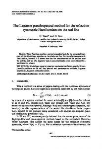
1. I N T R O D U C T I O N The numerical study of flow singularities is very important since they typically increase c o m p u t a t i o n a l errors. Singularities usually develop where the b o u n d a r y c o n t o u r is not smooth, such as at corners. A typical example is the viscous flow driven by the tangential m o t i o n of the top b o u n d a r y in a rectangular cavity (Fig. 1). The upper corners where the moving b o u n d a r y meets the stationary boundaries are singular points of the flow where the vorticity becomes u n b o u n d e d and the horizontal velocity is multivalued. The lower corners are also singular points, but are weaker in the sense that one more derivative is required to make a flow unbounded. The presence of singularities poses a particular problem for spectral J Department of Mechanical Engineering and Applied Mechanics, University of Michigan, Ann Arbor, Michigan 48109. z Currently at Korea Institute of Energy and Resources, Taejon, Korea. 3 Department of Atmospheric, Oceanic, and Space Science, and Laboratory for Scientific Computation, University of Michigan, Ann Arbor, Michigan 48109. 1 0885-7474/89/0300-0001506.00/0 9 1989 Plenum Publishing Corporation 854/4/1-1
2
Schultz et al. Ivl = i
(A, I)
I
//~2 F2
(-A, -i) Fig. 1. Problem schematic.
methods. These methods converge exponentially if a solution is infinitely differentiable (Gottlieb and Orszag, 1977), but singularities destroy the exponential convergence of the spectral coefficients. The errors caused by the singularity are typically spread over the entire solution domain in the form of Gibb's oscillations. As a result, most previous studies using spectral calculations avoid problems that have corner singularities. Instead they usually examine problems that have periodic boundary conditions in all but perhaps one direction--Fourier representations are used in the periodic directions and Chebyshev or Legendre polynomials in the other direction. For the Poisson equation with weak corner singularities, however, the double-Chebyshev spectral solutions (Haidvogel and Zang, 1979; Boyd, 1986) are still shown to be superior to the fourth-order finite difference method. The Chebyshev coefficients (amn) decay algebraically as (m +//)-6. The maximum pointwise error decreases more slowly as O(N 4) where N is the upper limit on the degree of the Chebyshev terms as expected for a two-dimensional series. In this paper we present a modified pseudospectral method that subtracts the strongest (inhomogeneous) singularities from the streamfunction. The sum of Chebyshev polynomials then represents a function that is only weakly singular. We test our approach on the driven cavity problem, which has been extensively studied using different numerical methods (Burggraf, 1966; Pan and Acrivos, 1976; Gupta, 1981; Ghia, Ghia, and Shin, 1982; Kelmanson,
Chebyshev PseudospectraIMethod
3
1983; Schreiber and Keller, 1983; Quartapelle and Naploitano, 1984; Ku and Hatziavramidis, 1985; Gustafson and Leben, 1986). The standard way to accommodate corner singularities in these nonspectral computational techniques is to use local mesh refinement. The two common methods of solving two-dimensional viscous flow problems use the stream function/vorticity or primitive variable formulations. A major difficulty posed by the stream function/vorticity formulation of the Navier-Stokes equation is the complexity of the vorticity boundary conditions. The primitive variable formulation, on the other hand, requires the pressure to be determined from a Poisson equation by taking the divergence of the momentum equation with an incompressibility constraint. The biharmonic equation for the stream function avoids the above difficulties (Schreiber and Keller, 1983) and also has the advantage of fewer unknowns--one-third the number of the primitive variable formulation and one-half that of the stream function/vorticity formulation for equivalent resolution. We begin this paper by presenting a modified pseudospectral method for the biharmonic equation for Stokes flow (zero Reynolds number), since the flow sufficiently close to a sharp corner is dominated by viscous terms. We then compute nonlinear flows in Section 4 to demonstrate that the modified method is also effective for small and moderate Reynolds number.
2. F O R M U L A T I O N In the absence of inertia, the steady-state flow of a viscous incompressible fluid in a rectangular cavity is governed by the Stokes equation. After scaling length and velocity by the half-depth and wall velocity, respectively, the governing equation and boundary conditions become
V4~] =0 ~b= q)x=0 = ~y=0
(2.1a)
o n x = _+A
(2.1b)
on y = - 1
(2.1c)
ony=l
2.1d)
and ~p=~by+ 1 = 0
where ~ is the dimensionless stream function. Equation (2.1d) implies that the upper boundary moves at unit velocity, while the other walls remain stationary. The only dimensionless parameter for this problem is the aspect ratio, A, which we choose to be unity for this study.
4
Schultz et al.
The analytical solutions for Stokes flow near singular corners have been obtained by Moffatt (1964). The singular solution 01), given in polar coordinates centered at the upper corners (see Fig. 1), is
Os(rl,
Os=rlf~(01)+ ~ bir~'+lfi(Oi)
(2.2)
The first term has the most important effect near the upper corners and is completely determined by the inhomogeneous boundary term in Eq. (2.1d). The other terms in the sum are less singular homogeneous terms with constants that must be determined globally. The singularities at the bottom corners are similar in form to Eq. (2.2) except that the inhomogeneous term is absent. To obtain excellent convergence properties for this problem, it is sufficient to account for the most singular term; hence, we will almost exclusively discuss results when only the most singular term is considered. If Os includes the other terms, the coefficients of the homogeneous singular functions (bi) must be included along with the spectral coefficients in the algebraic system. The general form of the functions fi(01) is
fl(O1)=AlcosOl+BisinOl+ClOlcosOl+DiOlsin01
(2.3a)
fi(01) = A; cos(2s + 1) 01 + B, sin(2s + 1) 01 + Ce cos(2i- 1 ) 01 + Di sin(2i- 1) 01
(2.3b)
Here, 2i are the complex eigenvalues in the first quadrant of the characteristic equation 2~ sin c~_+sin()~c~) = 0
(2.3c)
where c~ is the inner angle of the corner, in this case ~r/2. Constants A~, B~, Ci, and D~ are determined by the boundary conditions. These constants are complex except for i = 1. The boundary conditions (2.1b) and 2.1d) on x = - 1 , y = 1 can be rewritten as = Ox = 0
on 01 = n/2,
(2.4a)
and ~=0,
I~y+ 1 = 0
on01=0
(2.4b)
Using Eq. (2.2) and boundary conditions (2.4), we can write the form of the strongest corner singularity at both upper corners as
Os=rl[Ox(cosOl--2sinO1)--(2)2sinOll/(~---4--1)
(2.5)
Chebyshev PseudospectralMethod
5
Using the additional inhomogeneous and homogeneous singular basis functions of (2.2), we define an auxiliary stream function by ~1 = ~/a -I- ips,
(2.6)
where Os = Osl for this example (the homogeneous singular functions are ignored) and Oa is the stream function after the most singular behavior is subtracted throughout the entire solution domain. The unknown function Oa(x, y) is expanded as a truncated double Chebyshev series so that ~O(x, y) is approximated as N
~= ~
M
~ amnTn(x) Tm(y)+Os
(2.7)
n=0 m=0
Since (2.7) does not satisfy the boundary conditions, these must be imposed using the tau method. Lanczos (1964) presents a simple formula to determine the number of internal collocation points, PQ, in the x and y directions, respectively:
P=N+ 1-v
(2.8a)
Q = M + 1- v
(2.8b)
where v is the number of boundary conditions in each direction (two for second-order elliptic partial differential equations and four for fourthorder). The truncation shown in (2.7) has (N+ 1)(M+ 1) total degrees of freedom, so formulas (2.8) result in a deterministic system that is easily solved for all orders of one-dimensional differential equations and for twodimensional, second-order differential problems. The differential equation is applied on the internal collocation points and the boundary conditions are applied on the exterior points. For the two-dimensional, fourth-order differential equation, these formulas lead to an underdetermined system when a rectangular array of P by Q collocation points is used. Our attempts to make a determinate system using nonrectangular collocation arrays (i.e., adding more collocation points on the boundary) led to singular matrices. This is probably one reason why previous researchers have used the stream function/vorticity formulation. [Another possible method with the stream function formulation uses basis functions that satisfy the boundary conditions so that the tau boundary constraints are unnecessary. Although a rectangular array of collocation points leads to a determined system for this method, there are several algebraic complications (Zebib, 1984), especially for inhomogeneous boundary conditions.] In this paper we increase P and Q (usually by 1) resulting in a slightly overdetermined system, which must
6
Schultz
et aL
be solved in a least-squares sense. The internal collocation points are chosen to be the roots of the Chebyshev polynomial
x i= -cos
i = 1..... P = N - 2
(2.9a)
and yj=-cos
~
j = l ..... Q = M - 2
(2.9b)
Recognizing that V4O, = 0, we write the partial differential equation (2.1a) as ~=o m=o am,, ~x 4 Tn(xi) Tm(Yj) + 2 ~x 2 T,,(xi) +--5 Tm(Yj)
]
+ T,,(xi) dy---~ Tm(yj) = 0
(2.10)
The boundary conditions (2.1b)-(2.1d) are complicated by contributions of the singular stream function and its normal derivative: N
M
2
2 amn(+l)nTm(YJ)'+'l~s(+l, yj) =0
n=0 N
M
E
~ amnTn(Xi)('-}-l)m+l/Is(Xi, + 1 ) = 0
n-0
U n=0
(2.1 la)
m=0 (2.11b)
m=0
M ~ am~n2(+l) n•
d Tm(yj)+~x0,(_+l, yj)=0
(2.11c)
m=0
:v
M
n=0
m=0
d
F~ ~ am~rn(xi)m2+~y~',(x~,l)+ 1=o
(2.11d)
and N
2 n=0
M
2 amn Tn(xi) m2( m=0
-
-
1) m+1 + d 0s(xi, _ 1 ) = 0
(2.11e)
dy
where i = 1..... P, and j = 1,..., Q. We usually exclude the normal derivative boundary (2.11c)-(2.11e) at the four corners because of discontinuities in directions. However, when we apply the additional boundary that require both normal derivative boundary conditions to be corner, we have obtained a modest improvement in results.
conditions the normal constraints zero at the
Chebyshev Pseudospectral Method
7
Boyd (1989) introduces an effective method to evaluate the derivatives of the trigonometric functions using the transformation x = cos(t), which converts the Chebyshev series into a Fourier cosine series:
Tn(x) = cos(nt)
(2.12)
We have found that the derivatives computed this way are less susceptible to round-off errors than the more usual recurrence formulas. The derivatives of the Chebyshev polynomials are listed in the Appendix. The resulting overdetermined matrix problem is solved using a routine based on Householders' transformation (Golub, 1965). The cost is O(U2V) operations, where U is the number of unknowns and V is the number of equations. We have also tried a least-squares conjugate gradient iterative technique (Fletcher and Reeves, 1964), which solves the problem in O(UVI) operations, where I is the number of iterations. This method needed many iterations, however. Presumably, preconditioning would accelerate the convergence, although we did not experiment with preconditioning. 3. N U M E R I C A L RESULTS Table I summarizes calculations for the stream function at various truncations after subtracting the strongest singularity. The Stokes flow solution for a driven cavity is symmetric with respect to the x-axis. ThereTable I.
Stream Function Comparison r
M 5 7 9 11 Kelmanson 5 7 9 11 Kelmanson 5 7 9 11 Kelmanson
y
x=0
x=0.25
x=0.5
x=0.75
--0.5
0.03346 0.03332 0.03348 0.03348 0.0336
0.02886 0.02868 0.02890 0.02890 0.0290
0.01739 0.01715 0.01740 0.01740 0.0174
0.005303 0.005126 0.005215 0.005214 0.0052
0.0
0.1177 0.1177 0.1179 0.1179 0.1180
0.1037 0.1037 0.t039 0.1039 0.1040
0.06640 0.06641 0.06663 0.06664 0.0666
0.02202 0.02215 0.02224 0.02225 0.0222
0.5
0.1993 0.1996 0.1997 0.1997 0.1996
0.1836 0.1840 0.1840 0.1840 0.1840
0.1344 0.1350 0.1350 0.1350 0.1350
0.05510 0.05536 0.05537 0.05537 0.0554
8
Schultz et aL
fore, we reduce the number of grid points in the x-direction by a factor of 2 and examine the solution only on the domain 0 ~, 0
/ ,
(
9
I
/
~ - - - - - - - - - ~ -
........
r i i
-1 -1
-0.5
0
0.5
1
X
stream function
vorticity
Fig. 3. Streamlines (left) and vorticity lines (right) for computations with singular function. The streamline and vorticity contours are shown with the same increments as Fig. 2, except for negative streamfunction values with increments of 10 -6 to observe the largest Moffatt eddy in the lower corner.
10
Schultz et aL
system and because we did not introduce a similar coefficient for the upper corners. At any rate, as Gustafson and Leben (1986) show, even the largest Moffatt eddy can be described adequately by one singular coefficient. We find only minute differences between the computations shown in Fig. 4 and those of the first eigenfunction when the normalization is determined by a best fit given by D l = ( - 8 . 5 3 x 1 0 3 , - 1 : 5 5 1 x 1 0 2)/(21+1), where ),~ = (2.73959, 1.11902). A similar blow-up of an upper corner, Fig. 5, shows no eddies, as expected, since the strongest singular eigenfunction is not complex there. In Table II, the maximum value of the stream function within each eddy for our computations with 30 x 30 truncation is compared to those obtained by Pan and Acrivos (1976) and Gustafson and Leben (1986). The value of I//3 was determined from the local solution using the D 1 listed above. The stream function value of the corner eddies is in good agreement with those predicted by a scheme employing a local refinement and multigrid algorithm (Gustafson and Leben, 1986). The distance from the apex to the center of the first and second corner eddies d l / d 2 is 16.5 as in Gustafson and Leben, which is already in good agreement with the asymptotic result d~/d 2 = 16.4 obtained by Moffatt (1964) as r ~ 0.
-0.8
\,
-1
\
\ -0.8
x Fig. 4.
E n l a r g e m e n t of Moffatt eddies in lower corner. The streamline c o n t o u r s have the values - l x 1 0 -6 , - 2 x 1 0 -6 , - 3 x 1 0 -6, - 4 x 1 0 6, a n d - 4 . 4 x 1 0 6.
Chebyshev Pseudospectral Method
11
1
/ / / / / /
0.8
I'
0.8 X
Fig. 5.
E n l a r g e m e n t of u p p e r corner. The s t r e a m l i n e c o n t o u r s have the values 2 x 10 -2, lxl0 2, t x l 0 - 3 , a n d l x l 0 4.
Figure 6 shows the convergence of the inhomogeneous singular function spectral coefficients by expanding ~, as a double series of Chebyshev polynomials using pseudospectral methods. As expected, the coefficients (amn) converge algebraically at approximately order (m + n)-4 because the first derivative is discontinuous at the corners. Figures 7 and 8 show the pseudospectral coefficients of the driven cavity problem using a truncation of N = M = 29 (i.e., 30 x 30 truncation) with and without the most singular basis function, respectively. The coefficients appear to converge algebraically at a very large rate for both pseudospectral representations. The maximum coefficients for ~a (Fig. 7) are smaller by about a factor of 100 than for ~ itself (Fig. 8) for fixed n + m . Table II.
Vortex ~bI
~/2 03
Vortex Intensities
Pan and Acrivos
Gustafson a n d Leben
Present
0.2 --2.2 • 10 -6 6 . 6 x 1 0 -11
0.20012 - 4 . 4 6 • 10 -6 1 . 2 4 x 1 0 10
0.20014 - 4 . 4 5 4 • 10 -6 1.24 x l 0 10
10 ~
10 -I o o B
10 -2 ~
. o:O::~
I 0 -~
o':~ B:~ ~ ~
~
I 0 -4
*~
:o ~
~ 9 a o%1% o ,.*
10 -5
~
~ 1 ~7 6 1 7 6
10 -8 o ooo %
~
o o
oO
l
l
i 0 -7
10 .8
{
l
1
l
l
l i II
1oo
l
I
io'
]
l i i
io~
re+n+2 Fig.
6.
Convergence of the spectral coefficients of the inhomogeneous singular function. N=M=29. 10 0 10 -I o
10 -2 t
1 0 -~
o
a 9 oo ~
1 0 -4 Q
i 0 -5
D
oeD :
9 o
~o.:..
1 0 -a
o
9o l e a ~ 1 7 6 % ,S~
==
1 0 -v 10 -a 10 -9
Oo o ~
~
10-1o i0-11 10 -]2 i0 -13 I0 -14
ioo
i0 ~
10 ~
m+n+2
Fig. 7.
Convergence of the spectral coefficients for the driven cavity problem with singular function. N = M = 29.
Chebyshev Pseudospeetral Method
13
The rate of convergence of the coefficients is often used to infer the convergence of the solution, although some care is needed because the error usually decreases at a slower rate of convergence than the coefficients. We plot a collage of the bounded (i.e., maximum absolute value for fixed n + m) coefficient convergence for Fig. 6-8 on Fig. 9. In addition, we have plotted the bounded coefficients for the next most singular function in the upper c o r n e r bzr;a+]f2 with the coefficient b2 predicted by Kelmanson (1983). The spectral representation of b2/2 + lf2 exhibits faster convergence than the more singular inhomogeneous function, as expected; however, it is still slower than the coefficients from the solution for the entire driven cavity. This is caused by the different methods to obtain the coefficients: the coefficients in Fig. 7 are computed from an overdetermined algebraic system, as opposed to those for bzr;'Z+~f2. It is difficult to ascertain the convergence rates of the previous computations, in part because the coefficient convergence is opposite of that expected. One would expect a crossover point, where the exponential decrease of the spectral coefficients for the moderate n and m is replaced by the slower algebraic decay of the higher-degree coefficients as found in solving Poisson and Bratu equations with weak corner singularities (Boyd, 1986). Figures 7 and 8 show an I 0 -I i O -z *
o :o Oo
i O-a 10 -4
~ "Wr
I O-5 I 0 -e
~ o'b~o sg,
fi
,%.}
IO -v
.~176
1 0 -e
10 -9 i0 -Io
l0 -u 10 -12
I
lo ~
I
I
I
I
i
I TI
I
I
I
I
I
]
I l
lo' re+n+2
Fig. 8.
Convergence of the spectral coefficients for the driven cavity problem without singular function. N = M = 29.
Schultz et aL
14 101 i0 ~ '7
'7
w
10 -I
o o
o
v oo
o
I 0 -z
o
o ~ 8000%
--h 1 0 -3 N
oo;oN
10 -4
1 0 -5
~v
10 -8 o D
i 0 -v o ~ o o
c~
I 0 -a
% 10 -9
I
I
I
I
I
I
I II
td
I
l
I
I
I
I
I I
1of
m+n+2 Fig. 9. Convergence of spectral coefficients. Only the largest coefficient for fixed m + n is plotted. N = M = 2 9 . 9 Inhomogeneous singular function, rfl (Fig. 6); 9 driven cavity problem without singular function (Fig. 8); [~, driven problem with singular function (.Fig. 7); V, most singular homogeneous function, b2 ra'-+ 1f2.
increasing convergence rate at a crossover point that occurs near This appears to be due to the rectangular truncation (presumably larger coefficients for fixed m + n would occur for the small m or n not included in the truncation) and the nature of the overdetermined solution, as will be shown. The fourth derivative of the Chebyshev polynomial is proportional to n 4 as shown in the Appendix, hence the matrix components for Eq. (2.10) become larger as the truncation increases. Since terms are proportional to /It4 at the internal collocation points, we inadvertently weight the tau boundary constraints (which are of order n because they contain at most first derivatives) much less heavily. Therefore, we rescale the matrix, dividing each row by the maximum value of each row. Since we solve an overdetermined system, this scaling effectively changes the weighting of the least-squares procedure. The scaled equations then satisfy the boundary conditions with much higher accuracy and give a more accurate solution through the entire solution domain. Figure 10 shows the spectral coefficients for various truncations when
m+n+2=M.
15
Chebyshev Pseudospectral Method i0 ~ 0 0
10 -I
0
1 0 -2 O0
10 -a
QO
1 0 -4
Do
% 1 0 -5
o
c
o
IP
i 0 -s
gg i0 -v
I 0 -e 10 -9
o~
10 -1o o
10 -tl
o r
10 -12
o
u
o
10 -la
r
l
I
i
l I 111
10 0
m+n+2 Fig. 10. Convergenceof spectral coefficientssupplementing inhomogeneous singular function with and without using scaled matrix. Only the largest coefficient for fixed rn + n is plotted. 9 30 x 30 scaled matrix; ~, 16 x 16 scaled matrix; D, 16 x 16 unscaled matrix; V, 30 x 30 unscaled matrix. the driven cavity problem is supplemented by the inhomogeneous singular function with and without the scaled matrix. After subtracting the inhomogeneous singular functions the spectral coefficients amn using the scaled matrix show algebraic convergence with order (rn + n ) -8 like the Chebyshev expansions of the homogeneous and inhomogeneous singular functions of Fig. 9. The higher-order coefficients without the scaled matrix are damped out, as shown in Fig. 10, but those with the scaled matrix are not damped out by the least-squares procedure when we increase the truncation. This damping of the high-order coefficients with the least-squares procedure and the unscaled matrix decreases the solution accuracy, as explained below. For purposes of comparison of the solution convergence, we assume that the "exact" solution is given by the scaled matrix system using a 30 x 30 truncation, where the most singular term is subtracted, since no exact solution to the driven cavity problem exists. We must also determine a suitable definition of error, which should evaluate the error at other than the collocation points. We estimate an L2 error of ~ evaluated at a uniform
16
Schultz et al.
rectangular grid (including points on the boundary). The RMS error evaluated in this way increases with the number of evaluation points in the grid, since the convergence is not uniform due to larger errors near the singularities and boundary layers. However, the relative accuracy of different solutions is unaffected by the evaluation grid. Our error estimates are based on an 81 x 81 grid. A least-squares fit of the slope of the log-log plot in Fig. 11 shows that the error converges algebraically with the order of N 9 using the scaled matrix over the shown range of N + M when supplemented by the singular function. (The theoretical convergence rate could be quite different.) The convergence rate of the error is approximately N - 3 when the most singular function is not handled separately. Our computations indicate a convergence rate of N - 5 if the matrix is not scaled (not shown). We cannot show the exact convergence rate because the artificial "exact" solution does not allow the limit N ~ ~ . This may, in part, explain the surprisingly high convergence rate of error compared to the convergence rate of the coefficients. The convergence rate of the solution
10 -I
1 0 -2 10 -3 1 0 -4
i0 -s
10 -8 I 0 -7 i0 -s
i 0 -~ lo-tO
I
I
I I1[
I
10
I
1
l
I
I
I I
100
N Fig. 11. Convergence of driven cavity solution with truncation. The solution subtracting the inhomogeneous singular function with 30 • 30 truncation is considered the exact solution, tB, With singular function; A, without singular function.
L,
-- 1.46 x 10⁻⁵
-
4.2 x 10 7 1.93 x 10 - 7
7.5 • 10 - 7 1.63 • 1 0 -7
--0.3971725
-0.3971724
al,1 a7, io a7,14 E2
1.46 x 10⁻⁵
16
14
P
Scaled
T a b l e II1.
--0.3971727 - - 1 . 3 3 x 10 -5 1.1 x 1 0 - 6 6.33 x 1 0 - 7
18 --0.3971722 - - 3 . 4 4 x 10 6 5.4 x 10 - l ~ 2.02 x 10 5
14
C o n v e r g e n c e of the O v e r d e t e r m i n e d S y s t e m
2.15 • 10
2.11 • 10 5
5
-0.3971721 - - 2 . 8 6 • 10 6 - 4 . 6 x 10 -ix
18
--0.3971722 --3.03 x 10 - 6 - 6 . 7 x 10 11
16
Unscaled
Schultz et aL
18
should be lower than that of the coefficients by two orders. (Note that
k (m+n)k~O(N2-k)asN-+c~.) m = N n = N
It is interesting to see the effect of increasing the number of grid points (i.e., the number of equations) without changing the number of coefficients to check the convergence of a more highly overdetermined system. Table III shows that the convergence of the higher-order coefficients improves as the system becomes more overdetermined for the unscaled system; however, the error (compared to the "exact" solution described for Fig. 11) actually increases. The solution using the scaled matrix is more accurate than that of the unscaled matrix by factor of 50. This table indicates two things: that it is dangerous to make conclusions about the convergence of the solution from the convergence of the coefficients, and that it is more efficient to make the system as little overdetermined as possible. However, little additional error is introduced by making the system more overdetermined.
4. THE N O N L I N E A R P R O B L E M
We extend these techniques to small and moderate Reynolds numbers using the same inhomogeneous singular basis function, since the nature of the singular flow near the corner does not change when the nonlinear inertial terms are added. The Navier Stokes equations governing the steady flow of an incompressible viscous fluid can be written as V40 -
RGO = 0
(4.1)
where G is the nonlinear convection operator,
G~//=~ v2 ~l/] ax ~1//V2 ~x ~1/ (~y 1
(4.2)
and R is the Reynolds number. The no-slip boundary conditions are still (2.1b)-(2.1d). The unknown function 0(x, y) is still expanded as a truncated double Chebyshev series, adding the analytical form of the most singular function. We still overdetermine the problem using additional collocation points. The pseudospectral problem then leads to a nonlinear least-squares problem that is solved by a full Newton's method. This requires that a sequence of overdetermined linear problems be solved for Aamn, where
a(i+l)_ mn
--
(0 +Aamn
a rnn
(4.3)
Chebyshev PseudospectralMethod
19
and a~~ (the initial guess) is obtained either from a fully converged solution at lower Reynolds number or from a lower truncation solution at the same Reynolds number. We again solve for Aamn using the overdetermined scaled matrix that divides the matrix coefficients by the maximum value of each row. This scaling procedure is much more important than for Stokes flow, as the magnitude of the matrix elements for large N is of order N3R. The solution using the unscaled matrix diverges when the Reynolds number is large. Also, the driven cavity flow with inertia is no longer symmetric with respect to the x axis. Therefore, we must use both even and odd Chebyshev polynomials in both spatial coordinates. The iterated, overdetermined matrix equations are solved as before using a routine based on Householders' transformation (Golub, 1965). The Newton iteration of the algebraic nonlinear equations is robust. The procedure converges with amnCO) = 0 for large Reynolds numbers and small truncation, e.g., Re = 104 and N = 5. Increasing the spatial resolution increases the iteration convergence for high Reynolds number as expected. We also find that two procedures related to the overdetermined system speed up the Newtonian iteration convergence and enlarge the radius of convergence: weighting the boundary conditions and increasing the number of collocation points to further overdetermine the system. The results presented here use a boundary condition weighting of 103. That is, we use a second type of scaling: after making the maximum coefficient in each row equal to one as in Section 3, we multiply the rows representing the boundary tau constraints by 103. This also significantly improves the convergence of the solution error with respect to increased truncation N. The effect of making the system more overdetermined is less pronounced--its primary advantage is to increase the convergence radius. It has a very little effect on the solution error with respect to increased truncation N. Therefore, for the sake of computational efficiency, the results presented here are overdetermined as little as possible, i.e., P = N + 1 and Q = M + 1. Figure 12 show the lines of constant stream function with a stronger secondary vortex in the lower left corner for R = 100 using 30 x 30 truncation. The secondary vortices in the lower left corner become larger while those in the lower right corner diminish in size and, due to numerical errors, essentially "wash away." Similar figures for R = 50 and 200 are nearly identical to those of Ghia et aL (1982) (our Reynolds number is defined to be one-half those of others since our length scale is one-half the cavity depth). As the Reynolds number increases, nonphysical Gibbs oscillations appear near the wall. Ku and Hatziavramidis (1985) find Gibbs oscillations near R = 50. They show that these oscillations disappear when local expansions of the Chebyshev-spectral element method are employed. Our overdetermined procedure does not exhibit this problem until
20
Schultz et
aL
i
-0.5
[
-I
-0i.5
0
0.5
X
Fig. 12. The streamline contours for R = 100 are shown in increments of 0.02. The streamline
contours in the lower left corner are 0.0 and - 1 x 10⁻⁴.
significantly higher Reynolds numbers (R ,,~250) as long as the boundary conditions are weighted and the inhomogeneous singularity is subtracted to avoid the problem shown in Fig. 2. The vorticity values on the side walls near the upper corners of the driven cavity for 18 x 18 truncation and various R are shown in Table IV. We compare these values with those obtained using a perturbation solution (Gupta, Manohar, and Noble, 1981) and a finite difference method (Gupta, 1981) that are modified to fit our length scale. Our solution shows good agreement with the perturbation solution, especially for low Reynolds number. Since the perturbation procedure uses only the local solution, it is only valid in the limit as the distance from the corner goes to zero. Hence, the difference between the spectral and perturbation solutions is due to the less singular homogeneous terms that the perturbation procedure cannot take into account. The spectral results are considerably more accurate than the finite difference results, as indicated by the convergence data below. Table V shows the convergence of the vorticity near the upper corner on the stationary wall. Since the vorticity values near the corner are nearly singular, they converge slowly even though the Reynolds number is small. We obtain 5 digit (R = 0), 4 digit (R = 0.5), and 2 digit (R = 5) convergence
Chehyshev Pseudospectral Method
21
Table IV. Vorticity Values on the Stationary Walls: 18 x 18 Truncation R
(x, y)
Spectral
Perturbation
Finite difference
0
( - 1 , 0.9) (1, 0.9)
-13.6395 -13.6395
-13.6295 -13.6295
-9.04 -9.04
0.5
(--1, 0.9) (1, 0.9)
-13.693 -13.578
-13.67 -13.59
-9.07 -9.05
5
( - 1 , 0.9) (1, 0.9)
-14.2 -13.1
-14.02 -13.27
-9.27 -8.85
25
( - 1 , 0.9) (1, 0.9)
-16.3 -11.0
-15.91 -12.16
-9.27 -8.85
50
( - 1 , 0.9) (1,0.9)
-18.3 -8.7
-19.01 -11.52
-11.22 -7.53
using 18 x 18 truncation, shown in Table V. As might be expected from a global spectral method, the vorticity does not converge well at other locations, especially in the boundary layer near the moving wall. Kelmanson (1983) presents the homogeneous singular coefficients near the corner using a boundary integral method modified to account for the singularity in the Stokes flow problem (R = 0). Using his singular coefficients we estimate a vorticity value of -13.63918 at x = - 1 , y = 0 . 9 (Kelmanson defines vorticity with the opposite sign in his paper). Our solution (co = -13.63928) using 17 x 17 truncation agrees with Kelmanson (1983) to within five digits. Our solution should be more accurate because our solution for stream function gives 11 decimal accuracy (at 30x 30 truncation), but Kelmanson's gives only 4 decimal accuracy, as shown on Table I.
Table V. Convergence of Vorticity Values at x = - 1 , y = 0.9 Truncation
R= 0
R = 0.5
R= 5
R = 50
9x9 12 • 12 15 x 15 18 x 18 21 • 21 24 x 24 30 x 30
-- 13.6369 -13.6394 -13.6394 --13.6394 -13.6395 -13.6394 -13.6394
- 13.6435 -13.6648 -13.6841 -13.6936 -13.6905 --13.6788 -13.6730
- 13.04 --13.88 --14.08 -14.18 -14.15 -14.04 --
- 11.37 -12.93 -15.96 -18.28 -18.70 -17.82 --17.82
22
Schultz et al.
Figure 13 shows the spectral coefficients convergence for three different Reynolds numbers. A fit of Fig. 13 shows that the nonzero Reynolds number coefficients converge at the slower rate of ( n + m ) s. For sufficiently high Reynolds number, the nonlinearity rather than the singularity causes the slow convergence at this truncation, even though the nonlinear terms should not affect the asymptotic convergence limit (Boyd, 1986). We compare our results for velocity to those of Ghia et al. (1982) for R = 50 and 200. In spite of our lack of convergence of the vorticity at the corner (Table V), the vertical velocities for R = 50 at the cavity centerline are fully converged. A similar velocity profile with 2 6 x 2 6 truncation is indistinguishable from the results using 20 x 2 0 truncation. This would indicate that the results of Ghia et al. (1982) shown in Fig. 14 have not yet converged for their 129 x 129 or 258 x 258 grid. However, the convergence of the spectral results for R - - 2 0 0 is considerably slower. We do not know why this is so, but a plot of the spectral coefficients similar to those in Fig. 13 (not shown) shows a trend similar to those for R = 100 but with a sharp rise around n + m + 2 = 38. This indicates that the nonlinearity, and not the singularity, is causing the most computational difficulties.
i0 ~ D
10 -I
D
a
1 0 -2
Drn D
o
i0 -S
~
~
o oo
1 0 -4 o
10 -s 1 0 -6
~
o~ "~ o o ~
%
o ~
I 0 -v
%
o~
~
o o Oo o
1 0 -8
i0 -9 10 -1o
Oo o
10 -11
I
I
I
I
I I Ill
I
I
l
I
[
I
I I
io o
m+n+2 Fig. 13. Convergence of spectral coefficients for various Reynolds number (all truncation is 30x 30). 9 R=0; ~, R=I; D, R=100.
Chehyshev Pseudospectrai Method
23
0.4 0.3 0.2 0.1 0.0 -0.1
-0.2 -0.3
-0.4 I
I
-0.5 -
-0.5
0
0.5
X
F i g . 14.
V e r t i c a l v e l o c i t i e s a t t h e c a v i t y c e n t e r l i n e ( y = 0). - - , R = 50, N =
R = 50, N =
20 s p e c t r a l ;
O , R = 50, N =
129 finite d i f f e r e n c e ( G h i a
R = 200, N = 20 s p e c t r a l ; - - - - - , R = 200, N = 23 s p e c t r a l ; --
......
14 s p e c t r a l ; - - - - ,
et al., t 9 8 2 ) ; . . . .
,
, R = 200, N = 26 s p e c t r a l ;
, R = 200, N = 29 s p e c t r a l ; [3, R = 200, N = 129 f i n i t e d i f f e r e n c e ( G h i a et al., 1982).
5. CONCLUSIONS We presented a pseudospectral method supplemented by the analytic form of the corner singularity presented for two-dimensional Stokes flow problems using the stream function formulation. The method gives accurate solutions with far fewer grid points than higher-order finite difference and modified boundary integral methods. The rate of convergence for the pseudospectral coefficients and the error is greatly improved by subtracting the most singular part of the solution and using a scaled matrix. The overdetermined pseudospectral method proves to be simple to program, and is economical and very accurate. These techniques are extended to the solution of the driven cavity problem with inertia using the steam function formulation. The solutions are shown to be accurate for small and moderate Reynolds numbers using only 18x 18 truncation. These techniques are not well suited to the calculation of much thinner boundary layers because Gibbs oscillation may degrade numerical
24
Schultz et al.
accuracy. We recommend using a mapping or domain decomposition for high Reynolds number flows. ACKNOWLEDGMENTS This work was partially supported by the National Science Foundation under contracts Nos. MSM-8504456 and DMC-8716766 and partially by the Naval Research Laboratory under contract No. N00014-85-K-2019. REFERENCES Boyd, J. P. (1986). An analytical and numerical study of the two-dimensional Bratu equation, J. Sci. Comput. 1, 183-206. Boyd, J. P. (1989). Chebyshev and Fourier Spectral Methods, Springer-Verlag, New York. Burggraf, O. (1966). Analytical and numerical studies of the structure of steady separated flows, J. Fluid Mech. 24, 113-151. Fletcher, R., and Reeves, C. M. (1964). Function minimization by conjugate gradients, Comput. J. 7, 149-154. Ghia, U., Ghia, K. N., and Shin, C. T. (1982). High-Re number solutions for incompressible flow using the Navier-Stokes equation and a multi-grid method, J. Comput. Phys. 48, 231-248. Golub, G. (1965). Numerical methods for solving linear least squares problems, Numer. Math. 7, 206-216. Gottlieb, D., and Orszag, S. A. (1977). Numerical Analysis of Spectral Method. Theory and Applications, Society for Industrial and Applied Mathematics, Philadelphia. Gupta, M. M. (1981). A comparison of numerical solutions of convective and divergence forms of the Navier-Stokes equations for the driven cavity problem, J. Comput. Phys. 43, 260-267. Gustafson, K., and Leben, R. (1986). Multigrid calculation of subvortices, Appl. Math. Comput. 19, 89-102. Gupta, M. M., Manohar, R. P., and Noble, B. (1981). Nature of viscous flow near sharp corners, Comput. Fluids 9, 379-388. Haidvogel, D. B., and Zang, T. (1979). The accurate solution of Poisson equation by expansion in Chebyshev polynomials, J. Comput. Phys. 30, 167-180. Kelmanson, M. A. (1983). Modified integral equation solution of viscous flow near sharp corners, Comput. Fluids 11, 307-324. Ku, H. C., and Hatziavramidis, D. (1985). Solution of the two-dimensional Navier-Stokes equations by Chebyshev expansion method, Comput. Fluids 13, 99-113. Lanczos, C. (1964). Applied Analysis, Prentice-Hall, Englewood Cliffs, New Jersey. Moffatt, H. K. (1964). Viscous and resistive eddies near a sharp corner, J. Fluid Mech. 18, 1-18. Pan, F., and Acrivos, A. (1976). Steady flows in rectangular cavities, J. Fluid Mech. 28, 643-655. Quartapelle, L., and Naploitano, M. (1984). A method for the solving the factorized vorticitystream function equations by finite elements, Int. J. Num. Meth. Fluids 4, 109-125. Schreiber, R., and Keller, H. B. (1983). Driven cavity flows by efficient numerical techniques, J. Comp. Phys. 49, 310-333. Zebib, A. (1984). A Chebyshev method for solution of boundary value problems, J. Comput. Phys. 53, 443-455.