Checking Flight Rules with T RACE C ONTRACT Application of a Scala DSL for Trace Analysis Howard Barringer
Klaus Havelund
Robert A. Morris
University of Manchester, UK
Jet Propulsion Laboratory California Inst. of Technology, USA
NASA Ames Research Center, USA
[email protected]
[email protected]
[email protected]
Abstract Typically during the design and development of a NASA space mission, rules and constraints are identified to help reduce reasons for failure during operations. These flight rules are usually captured in a set of indexed tables, containing rule descriptions, rationales for the rules, and other information. Flight rules can be part of manual operations procedures carried out by humans. However, they can also be automated, and either implemented as on-board monitors, or as ground based monitors that are part of a ground data system. In the case of automated flight rules, one considerable expense to be addressed for any mission is the extensive process by which system engineers express flight rules in prose, software developers translate these requirements into code, and then both experts verify that the resulting application is correct. This paper explores the potential benefits of using an internal Scala DSL for general trace analysis, named T RACE C ONTRACT, to write executable specifications of flight rules. T RACE C ONTRACT can generally be applied to analysis of for example log files or for monitoring executing systems online. Categories and Subject Descriptors D.2.1 [Software Engineering]: Requirements/Specifications; D.2.4 [Software Engineering]: Software/Program Verification—Formal Methods, Programming by contract ; D.3.3 [Programming Languages]: Language Constructs and Features; D.2.5 [Software Engineering]: Testing and Debugging—Monitors General Terms Languages, Verification Keywords Scala, domain specific language, state machines, temporal logic, trace analysis, flight rules
1.
Introduction
Flight rules capture constraints that arise during NASA missions. They help mission operations teams to execute procedures correctly, thereby reducing the risk for failures. One particular form of flight rules concern commands sent from ground to a spacecraft or planetary rover during a mission. Such commands are sent in groups, called sequences (literally a sequence of commands). Each such sequence must
be verified against a fixed set of flight rules before being sent. Software is typically written in a rather ad-hoc manner to perform this verification, and a considerable challenge is managing the process by which system engineers express flight rules and constraints in prose, software developers translate these requirements into code, and both experts verify that the resulting application is correct. It would be an advantage if command sequence flight rules can be expressed in a formal notation that is (i) high-level, so that it can be understood by system engineers, and (ii) executable, so that conformance of a command sequence can be verified. We present an initial experiment on how to formalize flight rules for command sequences with a S CALA DSL (Domain Specific Language), called T RACE C ONTRACT [2], originally designed for general analysis of systems execution traces, that is: sequences of events, but here applied to sequences of commands (events and commands are technically both just data objects). The experiment has led to T RACE C ONTRACT, and S CALA, being chosen for command sequence verification for NASA’s LADEE (Lunar Atmosphere And Dust Environment Explorer) mission [21], scheduled for launch in 2012. As stated above, T RACE C ONTRACT generally supports analysis of traces, where a trace is defined as a sequence of events, without traversing the trace multiple times. An event in principle can be any form of data object, including for example commands. The DSL supports a notation allowing for a mixture of data parameterized state machines and temporal logic. The DSL can generally be used to analyze for example log files, or even monitor systems as they execute, and can in that context be seen as an extension of the principle of design by contract [24] (pre/post conditions and invariants) with trace predicates. The results presented in this paper should therefore be generally applicable to any trace analysis problem. A DSL can be developed as an external DSL or as an internal DSL. An external DSL is a stand-alone language, associated with a parser, that parses programs in the DSL and for example produces abstract syntax trees that can be processed by a host language. An internal DSL is essentially an extension of a host language, for example as an API. The
programming language S CALA [26] has convenient support for the definition of internal DSLs. T RACE C ONTRACT is an internal DSL. An advantage of an internal DSL is that the full power of the underlying host language is always available in case the defined DSL is not strong enough to handle a particular situation. A second advantage is the ease with which an internal DSL can be developed compared with developing an external DSL. Beyond not having to deal with parsing, this is mainly because many of the host language’s language features can be re-used as part of the DSL (examples are function definitions, parameterization, and pattern matching). This makes it easy to adapt the DSL and add new features. A third advantage is that one inherits all the tool support available for the host language, such as programming IDEs, debuggers, etc. Our previous studies have shown the potential benefits of internal DSLs based on P YTHON or S CALA to write executable specifications of monitor and control applications [7, 19]. A disadvantage of an internal DSL is the learning curve required by a user that is not normally programming in the host language. A large number of logics have been proposed in the past for analyzing execution traces. Most of these are external DSLs [1, 9, 11, 12, 17, 18, 20, 29]. T RACE C ONTRACT has evolved from our own previous attempts to develop external DSLs for trace analysis. These previous external DSLs include E AGLE [3, 10], RULER [4, 6] and L OG S COPE [4, 5]. The idea of embedding a trace analysis logic in a functional programming language has been tried before. Stolz and Huch describe in [30] an embedding of LTL (Linear Temporal Logic) in H ASKELL. Our framework differs in three ways. First, we handle data parameterization by reusing S CALA’s built-in notion of partial functions and pattern matching, similar to the way the Actor receive function is implemented in S CALA. Second, we introduce a hybrid between state machines and temporal logic. Third, the embedding in S CALA seems to provide notational advantages due to S CALA’s support for DSL development. Even ignoring the DSL for writing temporal properties, as a high level programming language, S CALA can be seen as an alternative to wide spectrum specification languages such as V DM ++ [13], R AISE [15], and A SML [16]. The rest of this paper is organized as follows. Section 2 provides an introduction to the design of a flight rule checker and presents an example set of flight rules, abstracted from three different NASA missions, that deal with the verification of command sequences. Section 3 presents the T RACE C ONTRACT DSL. Section 4 presents the formalization of the flight rules using T RACE C ONTRACT. Section 5 concludes with a discussion.
2.
Mission Flight Rules
2.1
Principles of Flight Rule Verification
Ground mission software comprises all ground software necessary to perform command and control of the spacecraft. A Ground Data System (GDS) supports all phases of the mission including development, test, and operations. Typical components of a GDS include those for telemetry and control, an alert system, one or more simulators, a flight dynamics system for orbit determination and design, a command sequencer, and a file and data management system. A GDS also consists of an engineering analysis suite of tools for analyzing the state of the spacecraft, and for verifying the GDS products that are uploaded to the spacecraft. One such tool, the focus of this paper, is the Flight Rule Checker. Flight rules comprise the primary operational document for a mission flight director and the supporting team responsible for conducting a space mission. Flight rules describe all the decisions to take in different flight situations. Flight rules are authored by system engineers and are usually assembled into a spreadsheet or database. Rules can be organized along many criteria, including: • Class or severity (from “safety/mission critical” to “pre-
ferred procedure”). • Subsystem to which rule is associated (for example, com-
munications, Guidance, Navigation and Control, Power System. • Mission phase of operation during which it is applicable. • Rule implementation, i.e., how the rule is to be applied
during operations. Different approaches to flight rule implementation include: • As a spacecraft software routine, in which the checks
occur as part of on-board processing. • As an operational procedure, implemented as checks or
warnings in command and flight procedures to ensure operator awareness. • Configured as limits or alerts into the mission command
and telemetry database. • Built into the ground data system (GDS) software to
check for errors. Some rules are implemented using more than one approach for added assurance through redundancy. For example, consider the following communications flight rule, which imposes a constraint on the warm-up time for a Traveling Wave Tube Amplifier (TWTA) prior to the transmission of data using a Ka modulator (transmitter). • Title: Ka-Band TWTA Turn-on. • Description: The TWTA shall be turned on 300 seconds
before turning on the Ka modulator. • Rationale: TWTA needs 300 seconds to warm-up.
• Implementation: Ops Procedures, Ground System Rule. • System: Communications. • Severity Class: B (Violation of this rule would result in
loss or degradation of measurement data required to meet full mission success. Minimum mission success criteria would still be met). • Mission phase: all.
An entry into the database will also contain a rule identifier for indexing and cross-referencing with other mission documents. 2.2
Command Sequence Verification
The focus here is on the verification of command sequences prior to being uploaded to the spacecraft. A command sequence is a sequence of low-level commands that is executed by the on-board controller. The command sequencer generates these sequences from high level tactical plans, produced by human or automated planners, that describe a sequence of science or engineering activities. The plans might be produced daily by the mission operations teams, or for multiple days. A command sequence is associated with a textual log that lists all the commands that were generated. Each command in the sequence log is a parameterized list of values describing the command. Among the fields are the type of command, the time at which the command is to start and its duration, and other fields as required. For example, a command called ‘set waypoint’ for changing the orientation of the spacecraft will include parameters describing the desired spacecraft attitude. The rule examples described below represent flight rules pertaining to the ordering and duration of commands in the command sequence log. Other kinds of rules might require a more expressive DSL than the one proposed below. For example, a flight rule such as “an instrument is never to be pointed into the sun” does not directly pertain to ordering or duration of commands, and may be better addressed through the use of a simulator. These scoping issues will be considered in future work. 2.3
Command Sequence Flight Rule Examples
Automated command sequence verification ensures the proper execution of commands by the on-board controller immediately prior to their upload. Violation of these rules would potentially put the spacecraft or its payload in danger, or inhibit the accomplishment of mission objectives. This section offers examples of flight rules from three different NASA missions (LCROSS [22], LRO [23] and LADEE [21]) that describe constraints on command sequences. Flight rules from multiple missions were examined in order to find common patterns among missions with otherwise different operations concepts and objectives. The selected rules are as follows.
Rules R1 R2 restrict the number and duration of commands in a sequence, which are imposed by the speed of the on board CPU. R1 : Command Rate “Operations shall limit commands to no more than 5 commands per second”. R2 : Command Granularity “No Stored Command Sequence shall include commands or command sequences whose successful execution depends on command time granularity of less than one second”. Rule R3 constrains a command to be executed only if a precondition that requires telemetry data is true. It prohibits an instrument to be powered on when the instrument is too cold (based on its current sensor reading). R3 : Command Precondition “Instrument shall not be powered on when any temperature sensor reads less than -20 ◦ C”. R4 is a constraint on the duration between the onset of a command to acquire a sun-pointing attitude (orientation in space) to the point where the spacecraft is fixed on that attitude. R4 : Command Minimum/Maximum Duration “The spacecraft shall acquire and maintain a sun-pointing attitude from an arbitrary attitude in no more than 30 minutes”. R5 imposes a wait duration on an Attitude Control System (ACS) command. It amounts to waiting for the ACS system to stabilize in a new state (mode) before issuing commands while in that mode. R5 : Duration-wait “ACS commands shall not be issued within 1 second of an ACS mode command”. R6 is the temporal ordering constraint explained in Subsection 2.1. R6 : Command Order timed sequence “The TWTA shall be turned on 300 seconds before turning on the Ka modulator”. R7 imposes a temporal exclusion constraint on commands. “Fine Point Mode” here refers to a state in which the spacecraft’s pointing control system is keeping the spacecraft precisely pointed and steady, for example in order to collect science data; the rule therefore restricts any ΔV maneuvers while in this state. R7 : Command Order concurrency/exclusion “No firing of main thrusters while spacecraft is in fine point mode”. Finally, R8 describes a set of spacecraft modes or states and the allowable transitions between them. For example, consider the three modes: SPM (Sun Point Mode), DB3
(Stellar Inertial Mode, deadband 3) and DB2 (Stellar Inertial Mode, deadband 2). These are all modes of the Attitude Control System. In LCROSS, SPM was a mode in which the solar arrays were pointed towards the sun. DB2 and DB3 enabled spacecraft ‘slew’ maneuvers of different precision, defined by an acceptable error bound called the ‘deadband’, which can be viewed as an imaginary box in space within which the spacecraft must be pointing (DB2 is more precise than DB3). Thus, the mode transition diagram restricts a transition from SPM to DB2, forcing a mode change to DB3 first. R8 : Mode Transition “Mode and submode transitions shall be restricted to the set represented in the state transition diagram in Figure 1 under nominal flight operations”.
Figure 1. Requirement R8 : allowed mode transitions.
2.4
The use of M ATLAB to Formalize Flight Rules
Figure 2 shows a M ATLAB formulation of requirement 7. M ATLAB has been used for command sequence verification in past missions. The code consists of initializing a text verification report summarizing the result of applying the rule to an input consisting of the sequence log. The body of the code consists of checking for any occurrence of a set mode command that puts the spacecraft into fine point mode. If such a command is observed, then the remainder of the code checks to insure that no fire main thruster command occurs before the spacecraft transitions out of fine point mode. If a violation of this constraint occurs, an error report is generated. Many flight rules pertaining to command sequences have similar patterns, namely, the requirement that certain preconditions be true prior to the execution of the commands. The existence of these patterns suggest that flight rule verification can be formalized using a domain specific language (DSL). The remainder of this paper proposes the use of a general trace analysis DSL for this purpose.
function vreport = ChkNoBurnDuringPtMode(inputs) vreport = strcat(10, 10, ’Report Summary for Flight Rule ChkNoBurnDuringPtMode’); vreport = strcat(10, ’This rule checks to ensure that no main thruster firings occur during fine point mode’); vreport = strcat(vreport, 10, ’************’); i = 1; sum = 0; mode = 0; s = size(inputs.log); c = s(2); while i < c if strcmp(inputs.log(i).cmd, ’SET_MODE’) mode = inputs.log(i).acs_mode; set = i; else if strcmp(inputs.log(i).cmd, ... ’FIRE_MAIN_THRUSTER’) && mode ==2 sum = sum +1; vreport = strcat(vreport, 10, ’Check fails’); vreport = strcat(vreport, 10, ’Reason: FIRE_MAIN_THURSTER at line ’, num2str(i), ’ was attempted while in Fine Point Mode’); end end i = i+1; end vreport = strcat(vreport, 10, ’************’); vreport = strcat(vreport, 10, ’Summary Report:’); if sum == 0 vreport = strcat(vreport, 10, ’All tests on input log file passed’); else vreport = strcat(vreport, 10, ’Input log violates the flight rule test ’, num2str(sum), ’ times.’); end end
Figure 2. Requirement 7 in M ATLAB: No firing of main thrusters while spacecraft is in fine point mode.
3.
The T RACE C ONTRACT DSL
3.1
Motivation and Context for T RACE C ONTRACT
T RACE C ONTRACT is a S CALA package for analyzing traces. A trace is a sequence of events, for example emitted from a running system that we want to monitor. T RACE C ONTRACT is a solution to the following problem: “Develop a DSL in which one can specify and monitor requirements about sequences of events. The DSL should be as succinct as possible, while at the same time being as expressive as possible”.
An important design goal has been to produce a very expressive DSL, able to handle realistic real-life properties, while incorporating useful notations such as state machines and temporal logic. We observe that we would want to be able to monitor the events as they are produced. Hence, we do not assume that we have all the events available. However, when processing a log, we do have all the events available. Our solution should be flexible to support both these scenarios. Our solution is a generalization of state machines adding the following concepts: • states can be parameterized with data. • there are different kinds of states inspired by temporal
logic operators. The operators differ wrt: how they react to events that do not trigger transitions. how they behave at the end of the trace. That is, whether they evaluate to True or False. whether they remain active after a transition is taken. • un-named (anonymous) states are allowed, thereby re-
import tracecontract.Monitor // Define events: abstract class Event case class COMMAND(name: String) extends Event case class SUCCESS(name: String) extends Event case class FAIL(name: String) extends Event // Define monitor: class CommandRequirements extends Monitor[Event] { property(’R1) { always { case COMMAND(name) => hot { case FAIL(‘name‘) => error case SUCCESS(‘name‘) => ok } } }
lieving the user from naming intermediate states in a progression of transitions.
property(’R2) { always { case SUCCESS(name) => state { case SUCCESS(‘name‘) => error case COMMAND(‘name‘) => ok } } }
• the target of a transition can be a conjunction (AND) of
states as well as a disjunction (OR), corresponding to alternating automata. These characteristics makes the DSL appear as a combination of state machines and temporal logic, making it a well suited notation for specifying requirements. The fact that they can be mixed with S CALA code, with side effects, means that T RACE C ONTRACT is a very succinct and expressive specification DSL. 3.2
A Complete Self-Contained Example
We shall illustrate T RACE C ONTRACT with a complete, selfcontained example. Figure 3 shows what a user of T RACE C ONTRACT might write to monitor telemetry between a control center and a spacecraft. Note that although monitoring telemetry is not exactly the same as monitoring command sequences, the similarities are sufficient to justify using the former as an example here. The first task to perform is to determine what the events are to be monitored. T RACE C ON TRACT allows for events to be of any S CALA type, but the usual way is to define event kinds as parameterized case classes (to allow for pattern matching), all subclassing an abstract Event class. The example shows the definition of 3 kinds of events representing: (i) sending a named command to the spacecraft, and observing (ii) its success or (iii) its failure. Next, we define a monitor, which defines the two properties. A monitor is a class that extends the Monitor class, which itself is parameterized with the event type. The Monitor class offers all the classes and functions provided for writing trace contracts. The monitor defines two properties, named ’R1 and ’R2, corresponding to the requirements:
} // Use monitor: object TraceAnalysis { def main(args: Array[String]) { val trace: List[Event] = List( COMMAND("STOP_DRIVING"), COMMAND("TAKE_PICTURE"), SUCCESS("STOP_DRIVING"), SUCCESS("STOP_DRIVING")) val monitor = new CommandRequirements monitor.verify(trace) } }
Figure 3. A complete example. • R1 : An issued command must eventually succeed without
a fail occurring first. • R2 : A command cannot succeed more than once before a
new with the same name is issued. Property ’R1 reads as follows: it is always the case that, if a COMMAND(name) is observed, then we enter a new (un-
named) state (which is hot, meaning we need to exit it eventually), where if we see a FAIL(‘name‘) it is an error, until we see a SUCCESS(‘name‘). The quotes around ‘name‘ means: “match the value of name”. Property ’R2 reads as follows: it is always the case that, if a SUCCESS(name) is observed, then we enter a new state, where if we see another SUCCESS(‘name‘) it is an error, unless we see a new COMMAND(‘name‘). The TraceAnalysis class shows how the monitor is used. First we create a trace, which is a list of events of the Event type. Such a trace will of course typically come from somewhere outside the monitoring program, for example as a result of reading a log file. Then we create an instance of the CommandRequirements monitor, and finally call the verify method on the monitor, with the trace as argument. The result of running this program is shown below: *** Safety error: Monitor: CommandRequirements Property ’R2 violated Violating event number 4: SUCCESS(STOP_DRIVING) Error trace: 3=SUCCESS(STOP_DRIVING) 4=SUCCESS(STOP_DRIVING) *** Liveness error: Monitor: CommandRequirements Property ’R1 violated - missing event Error trace: 2=COMMAND(TAKE_PICTURE) Two errors are shown, one showing that requirement R2 is violated due to two successes of the STOP_DRIVING command (a so-called safety error) and one showing that requirement R1 is violated due to a missing success of TAKE_PICTURE (a so-called liveness error). For each error an error trace is printed showing the events involved in causing the error (missing events are not shown in these error traces). 3.3 3.3.1
abstract class Formula { def apply(event: Event): Formula def reduce(): Formula = this def and(that: Formula): Formula = And(this, that).reduce() def or(that: Formula): Formula = Or(this, that).reduce() ... }
The apply function allows one to apply a formula f to an event e as follows: f (e), resulting in a new formula. The core idea is the following: for each new event, each formula is evaluated by applying it to each new event, to become a new formula.This new formula may be one of the formulas False or True, or some derivation of the original formula. The function is defined as abstract and is overridden by the different subclasses of Formula corresponding to the various kinds of formulas available. The reduce function will rewrite the formula according to the classical reduction axioms of propositional logic (for example true ∧ f = f for any formula f ). It will be overridden in subclasses of Formula. Methods like ‘and’ and ‘or’ allow us to construct conjunction and disjunction of formulas using infix notation. That is, given two formulas f1 , f2 , the function ‘and’ allows us to write: f1 and f2 , a syntax supported by S CALA instead of the more classical (also allowed): f1.and(f2). In the case of f1 and f2 , the result is an object of class And, which is a subclass of Formula: case class And(formula1: Formula, formula2: Formula) extends Formula { override def apply(event: Event): Formula = And(formula1(event), formula2(event)).reduce() override def reduce(): Formula = { (formula1, formula2) match { case (False, _) => False case (_, False) => False case (True, _) => formula2 case (_, True) => formula1 case (f1, f2) if f1 == f2 => f1 case _ => this } }
Under the Hood of T RACE C ONTRACT Fundamentals
In this section the implementation of T RACE C ONTRACT will be outlined. For the explanation we shall assume a type of events (in the above example in Figure 3 the abstract class Event): type Event
A monitor consists of a collection of properties. A property is a named formula, defined with the method: def property(name: Symbol)(formula: Formula): Unit
The type Formula represents our formulas, and is modeled as an abstract class of which various formulas will form subclasses (as when defining an abstract syntax):
}
A term such as And( f1 , f2 ) is evaluated by evaluating its subformulas, and subsequently calling reduce to perform propositional logic reduction. The atomic formulas are True, False, and Now(e), for some event e. The latter formula is true if the current event is equal to e:
case object True extends Formula { override def apply(event: Event): Formula = this } case object False extends Formula { override def apply(event: Event): Formula = this } case class Now(expectation: Event) extends Formula { override def apply(event: Event): Formula = if (expectation == event) True else False }
The functions error and ok are with a simplified view just representing False and True (they are actually functions that in the case of error, for example, produces an error message). Versions also exist that take user defined messages as arguments, which get printed. Each of the three functions always, state, and hot produces a formula, which at some level behaves like a state in a state machine, although with additional twists. Each of the functions take as argument a partial function from events to formulas, also called a block. A block can be thought of as representing the transitions leading out of the state. S CALA allows us to write a partial function as a sequence of case statements, as in: {
An event can occur in a position requiring a formula due to the following implicit conversion function:
case FAIL(‘name‘) => error case SUCCESS(‘name‘) => ok }
implicit def convEvent2Formula(event: Event): Formula = Now(event)
There are other conversion functions, for example converting Boolean values and the Unit value to Formulas, the latter being useful for allowing code with side effects as part of state machines: implicit def convBoolean2Formula(cond: Boolean): Formula = if (cond) True else False implicit def convUnitToFormula(unit: Unit): Formula = True
3.3.2
States
In the specification above, property R1, as an example, consists of the formula: always { case COMMAND(name) => hot { case FAIL(‘name‘) => error case SUCCESS(‘name‘) => ok } }
This formula, and the formula for R2, are constructed using the following five functions from the DSL: def error = False def ok = True type Block = PartialFunction[Event, Formula] def always(block: Block): Formula = Always(block) def state(block: Block): Formula = State(block) def hot(block:Block): Formula = Hot(block)
As already mentioned, different states behave differently wrt. how they react to events that do not trigger transitions, whether they remain active after a transition is taken or not, and how they behave at the end of the trace. The semantics of the different states Always, State and Hot, plus for some other states not mentioned so far, are shown below. Each kind of state forms a subclass of class Formula: case class Always(block: Block) extends Formula { override def apply(event: Event): Formula = if (block.isDefinedAt(event)) And(block(event),this) else this } case class State(block: Block) extends Formula { override def apply(event: Event): Formula = if (block.isDefinedAt(event)) block(event) else this } case class Hot(block: Block) extends Formula { override def apply(event: Event): Formula = if (block.isDefinedAt(event)) block(event) else this } case class Step(block: Block) extends Formula { override def apply(event: Event): Formula = if (block.isDefinedAt(event)) block(event) else True } case class Strong(block:Block) extends Formula{ override def apply(event: Event): Formula =
if (block.isDefinedAt(event)) block(event) else False } case class Weak(block: Block) extends Formula { override def apply(event: Event): Formula = if (block.isDefinedAt(event)) block(event) else False }
Consider the Always class. The apply method returns “itself” (this) in case the body block of transitions is not defined for the event (no transition matches). This represents the semantics that we stay in the state in this case. On the other hand, if the block is defined for the event, the block is applied (a transition is taken), resulting in a new formula. This resulting formula is now monitored together with the original always state by anding them together (And). The other states are left once a transition is taken, as in traditional state machines. These states differ in how they treat the case where a current event does not trigger a transition, and in how they behave at the end of the trace. Some of the states behave identically wrt. how they handle nontriggering events (State behaves as Hot and Strong behaves as Weak), but these states are then distinguished by how they evaluate at the end of the trace. The following function (only partially shown) is called at the end of the trace and evaluates each formula at that point to either false or true (false if something should have happened but did not): def end(formula: Formula): Boolean = formula match { case True => true case False => true case Now(_) => false case And(formula1, formula2) => end(formula1) && end(formula2) case Or(formula1, formula2) => end(formula1) || end(formula2) case Always(_) => true case State(_) => true case Hot(_) => false case Step(_) => true case Strong(_) => false case Weak(_) => true ... }
3.3.3
The Verify Methods
The example in Figure 3 illustrates the application of a verify function that takes a trace as argument: def verify(trace: List[Event]): MonitorResult[Event]
The following set of alternative functions are furthermore provided for verifying events one by one, for example when monitoring a system online: def verify(event: Event): Unit def end(): Unit
The end function must be called at the end of the event sequence. A monitor can define one or more properties, and monitors can be composed. It is a matter of taste whether one or more properties should be defined in a monitor. For our examples we shall define each monitor to contain one property. As an abbreviation, properties can be defined with the following function (calling a version of property that only takes a formula as argument, no name): def require(block: Block): Formula = property(always(block))
3.3.4
Other Forms of Specification
The DSL also supports writing Linear Temporal Logic (LTL) formulas [25], such as: globally { COMMAND("STOP_DRIVING") implies eventually(SUCCESS("STOP_DRIVING")) }
and even a mixture of states and LTL, which allows pattern matching on events to capture data: always { case COMMAND(x) => eventually(SUCCESS(x)) }
The framework also supports a rule-based framework for recording facts, useful for checking past time properties.
4.
Formalizing Flight Rules
This section presents the formalization in T RACE C ON TRACT of the requirements informally described in Section 2. First we need to formalize what events are. Subsequently each requirement is formalized. 4.1
Events
Two kinds of events are considered: commands submitted to the spacecraft, and status updates from the spacecraft1 . The type Event of events and the two different kinds of events are defined in Figure 4. Each event has a time stamp. A command has a name, a value, a time stamp (when the command is issued), and a deadline by which it should be executed. A status update has a name (what kind of status 1 Even though the intended application in the LADEE project is a command sequence checker, we have performed experiments with analyzing telemetry such as status updates.
update is it), an identity (for example the id of a sensor), a value, and a time stamp.
def def def def def
abstract class Event { val time: Int } case class COMMAND( name: String, value: Any, time: Int, deadline: Int) extends Event
}
class R1 extends Monitor[Event] { require { case COMMAND(name, _, time, _) if name startsWith "ATS" => count(time) }
case class STATUS ( name: String, which: String, value: Int, time: Int) extends Event
def count(time: Int, nr: Int = 1): Formula = state { case COMMAND(name, _, time2, _) if name startsWith "ATS" => if ((time,time2) beyond (1 second)) ok else if (nr == 5) error else count(time, nr + 1) }
Figure 4. The type of events. 4.2
Requirement 1
Requirement R1 is formalized in Figure 5. The formalization states that whenever (recall that require(f) = property(always(f))) we observe a command whose name starts with ATS, we enter a state returned by the count function, which for the next 1 second counts the number of ATS commands. When an ATS command is observed with a time stamp beyond 1 second, we stop monitoring this particular sequence (ok). If this number, however, before that exceeds 5, an error is issued. The technique of using a function (here count) to represent a named state is also used to represent more traditional state machines, see requirements R6 in Figure 10, and R8 in Figure 12. The “machinery” behind the expression: (time,time2) beyond (1 second)
is the following implicit conversion functions and classes2 : implicit def convIntPair2IntPairOps(pair: (Int, Int)) = new IntPairOps(pair._1, pair._2) class IntPairOps(x: Int, y: Int) { def within(z: Int) = (y - x) z } implicit def convInt2IntOps(x: Int) = new IntOps(x) class IntOps(x: Int) { def second : Int = x * 1000 2 This is not a crucial part of the T RACE C ONTRACT DSL. If nothing else, it illustrates how implicit functions can be used to define a DSL.
seconds : Int = second minute : Int = x * 60 * 1000 minutes : Int = minute hour : Int = x * 60 * 60 * 1000 hours : Int = hour
}
Figure 5. Requirement 1: Operations shall limit ATS and RTS commands to no more than 5 commands per second. 4.3
Requirement 2
Requirement R2 is formalized in Figure 6. It is a check on arguments to individual commands. The partial function argument to the function require returns the Boolean expression: “(time,deadline) beyond (1 second)”. This Boolean expression, occurring as the “target of a transition” (using state machine terminology), is lifted to a formula by the implicit definition: implicit def convBoolean2Formula(cond: Boolean): Formula = if (cond) True else False
class R2 extends Monitor[Event] { require { case COMMAND(_, _, time, deadline) => (time,deadline) beyond (1 second) } }
Figure 6. Requirement 2: No Stored Command Sequence shall include commands or command sequences whose successful execution depends on command time granularity of less than one second.
4.4
Requirement 3
Requirement R3 is formalized in Figure 7. The property states that if a temperature reading (STATUS("TEMP",...)) is observed, with a temperature less than −20 ◦ C, then we enter a state in which a POWERON command results in an error. However, if in this state a reading of the same sensor yields a temperature bigger than or equal to −20 ◦ C, the observation of this sensor stops (ok). Note that several temperature sensors could go below −20 ◦ C. They would all have to go back ≥ −20 ◦ C before a POWERON is safe. The formalization keeps track of all sensors. class R3 extends Monitor[Event] { require { case STATUS("TEMP",sensor, value, _) if value < -20 => state { case COMMAND("POWERON", _, _, _) => error case STATUS("TEMP",‘sensor‘, value2, _) if value2 >= -20 => ok } } }
Figure 7. Requirement 3: Instrument shall not be powered on when any temperature sensor reads less than −20 ◦ C. 4.5
Requirement 4
class R5 extends Monitor[Event] { require { case COMMAND("ACS_MODE", _, time1, _) => state { case COMMAND("ACS", _, time2, _) if (time1,time2) within (1 second) => error } } }
Figure 9. Requirement 5: ACS commands shall not be issued within 1 second of an ACS mode command. 4.7
Requirement R6 is formalized in Figure 10. This requirement is formalized as a state machine with two states: the initial Init state, and the On state parameterized with the time at which a “turn on TWTA” command occurs. The state machine transitions to the On(time) state if TWTA is turned on at time. In the On state we have to wait at least 300 seconds before a command turning on KA is allowed. Note that we provide the return type Formula explicitly for the functions Init and On. Explicit mentioning of return types for mutually recursive functions is required by S CALA’s type system (although not for all functions involved). class R6 extends Monitor[Event] { property { Init }
Requirement R4 is formalized in Figure 8. The formalization illustrates the use of a hot state: when a command is issued to point to the sun, then a hot state is entered. This means that eventually a status update must be observed that the spacecraft is sun pointing. Furthermore, the only release of this obligation (result: ok) is if a status update arrives within 30 minutes. class R4 extends Monitor[Event] { require { case COMMAND("SUN_POINTING", _, time1, _) => hot { case STATUS("SUN_POINTING", _, _, time2) if (time1, time2) within (30 minutes) => ok } } }
Figure 8. Requirement 4: The spacecraft shall acquire and maintain a sun-pointing attitude from an arbitrary attitude in no more than 30 minutes. 4.6
Requirement 5
Requirement R5 is formalized in Figure 9. This is another example illustrating how real-time constraints can be expressed.
Requirement 6
def Init: Formula = state { case COMMAND("TURNON", "TWTA", time, _) => On(time) case COMMAND("TURNON", "KA", _, _) => error } def On(twtaTime: Int): Formula = state { case COMMAND("TURNOFF", "TWTA", _, _) => Init case COMMAND("TURNON", "KA", kaTime, _) if (twtaTime,kaTime) within (300 seconds) => error } }
Figure 10. Requirement 6: The TWTA shall be turned on 300 seconds before turning on the Ka modulator. 4.8
Requirement 7
Requirement R7 is formalized in Figure 11. The formalization states that if mode is set to 2 (fine point mode), with a SET_MODE command, then we enter a state where a FIRE_MAIN_THRUSTER command is not allowed. We leave that state again as soon as the mode is set to a value dif-
ferent from 2. The reader may compare this formalization with the M ATLAB formalization in Figure 2. The comparison is not quite fair due to the fact that the M ATLAB program contains several lines concerned with counting and printing. However, our DSL does all this automatically for us. class R7 extends Monitor[Event] { require { case COMMAND("SET_MODE", 2, _, _) => state { case COMMAND("SET_MODE", x, _, _) if x != 2 => ok case COMMAND("FIRE_MAIN_THRUSTER", _, _, _) => error } } }
def SPM: Formula = state { case COMMAND("MOVETO", "DB3", _, _) => DB3 case COMMAND("MOVETO", _, _, _) => error }
This state will wait for a MOVETO command to appear, in which case one of the two transitions will be taken.
class R8 extends Monitor[Event] { select{case COMMAND("MOVETO",_,_,_) => true} property { SPM } def SPM: Formula = weak { case COMMAND("MOVETO", "DB3", _, _) => DB3 }
Figure 11. Requirement 7: No firing of main thrusters while spacecraft is in fine point mode. 4.9
def DB1: weak { case case case case }
Requirement 8
Requirement R8 is formalized in Figure 12. The formalization faithfully models the state machine shown in Figure 1. Each state is represented by a function (SPM, DB1, etc). Note, however, that in contrast to the previous state machines, in particular the one for requirement R7 in Figure 11, the states in this state machine are weak. Recall that the semantics of a weak state is the following: the next event has to match one of the transitions, otherwise it is an error. However, if there is no next event, a weak state evaluates to True. In other words: if there is a next event, it has to match one of the transitions in the current state. If we monitored a command sequence against this state machine we would likely get a violation since not all events are likely to be MOVETO commands. However, the select function (called in the first line of the monitor) ensures that only events matching COMMAND("MOVETO",_,_,_) are processed by this monitor. The select function has the following signature:
def DB2: weak { case case case }
"SLM", "DB2", "DB3", "DVM",
_, _, _, _,
_) _) _) _)
=> => => =>
SLM DB2 DB3 DVM
Formula = COMMAND("MOVETO", "SLM", _, _) => SLM COMMAND("MOVETO", "DB1", _, _) => DB1 COMMAND("MOVETO", "DB3", _, _) => DB3
def SLM: Formula = weak { case COMMAND("MOVETO", "DB2", _, _) => DB2 case COMMAND("MOVETO", "DB3", _, _) => DB3 }
The filter provided as argument to the function is used to select events to be processed by the monitor. That is, only events e for which:
are submitted to the monitor for analysis. Note that without such a selection, we would have to use for example the state function and provide error transitions. For example, the SPM state would become:
COMMAND("MOVETO", COMMAND("MOVETO", COMMAND("MOVETO", COMMAND("MOVETO",
def DB3: Formula = weak { case COMMAND("MOVETO", "DB2", _, _) => DB2 }
def select(filter: PartialFunction[Event, Boolean]) : Unit
filter.isDefinedAt(e) && filter(e)
Formula =
def DVM: Formula = weak { case COMMAND("MOVETO", "DB3", _, _) => DB3 } }
Figure 12. Requirement 8: Mode and submode transitions shall be restricted to the set represented in the state transition diagram in Figure 1 under nominal flight operations.
4.10
Monitoring the Requirements
T RACE C ONTRACT allows us to construct monitor hierarchies, useful for composing monitors. The requirements defined above can be composed into the monitor Requirements shown in Figure 13. class Requirements extends Monitor[Event] { monitor ( new R1, new R2, new R3, new R4, new R5, new R6, new R7, new R8 ) }
Figure 13. Requirement composition. This monitor can now be applied to analyze a trace. Figure 14 shows a concrete analysis. The Requirements monitor is first instantiated to an object with the name monitor. An example trace is then provided as argument to the monitor’s verify method. Normally the trace would likely get read in from a log file for example. object Analysis { def main(args: Array[String]) { val monitor = new Requirements val log = List( // example log COMMAND("MOVETO", "DB3", 1000 , COMMAND("MOVETO", "DB2", 5000 , COMMAND("MOVETO", "DVM", 10000, COMMAND("MOVETO", "DB3", 15000, monitor.verify(log) } }
3000), 7000), 12000), 17000))
Figure 14. Requirement Analysis.
5.
Discussion
We have presented T RACE C ONTRACT, an internal S CALA DSL for trace analysis, and demonstrated its application for writing flight rules. T RACE C ONTRACT, as well as the conclusions from this work, are applicable to general forms of trace analysis, including, for example, analysis of log files or monitoring of running systems. The technology and lessons learned are not specific to flight rules. A main question is whether a trace analysis DSL should be an external or an internal DSL. An internal DSL has the following advantages: expressive power due to the fact that the host language, in this case S CALA, is part of the DSL; ease of implementation, and thereby ease of adaptation to user requests; and inheritance of tool support for the host language. Furthermore, S CALA is a high level programming language, and in itself seems very suited for writing executable specifications.
An internal DSL is usually associated with the following disadvantages: the notation may not be optimal for the specific problem; complexity of DSL since it includes a programming language; and lack of analyzability. Lack of analyzability means that it is difficult to analyze a specification from within the host language (in this case S CALA) - it may require compiler plugins. This can have consequences for performance and reporting to users. This is specifically the case where the DSL is a shallow embedding in the host language S CALA. This means that we re-use as many of S CALA’s language constructs, including for example functions, case classes and pattern matching. This is in contrast to a deep embedding where the host language’s constructs are not part of the DSL. A discussion of advantages and disadvantages of these two approaches is presented in [14]. It is too early from our experience on the LADEE mission to determine whether flight rule specification and checking provide a good application of an internal DSL using S CALA and T RACE C ONTRACT. However, we have in the past made experiments with external (as well as internal) DSLs for trace analysis, and can at this point make some observations. One such external DSL is L OG S COPE [4, 5], which grew out of the RULER external DSL for trace analysis [4, 6]. RULER and T RACE C ONTRACT have the same formal expressiveness, and are both more expressive than L OG S COPE. L OG S COPE was developed to help JPL engineers analyze log files. L OG S COPE is simple compared to T RACE C ON TRACT, and therefore easy to learn. We consider the advantages of an internal DSL for trace analysis to outweigh the disadvantages. We consider expressive power (and availability of a high level programming language) and ease of implementation to be the most important aspects. Ease of implementation means that it is not crucial whether the DSL is perfect from the start. It can evolve easily as experience is gained. Although the S CALA DSL in some cases does not become as succinct as an external DSL (for example, in an external DSL one would probably omit the case keyword in transitions), it seems to come sufficiently close to the ideal. The main potential disadvantage is the complexity of the DSL, that a user has to be a S CALA programmer. It is difficult to make a general statement here, but we believe that for writing effective trace analyzers, one needs a powerful formalism, extending a high level programming language, such as T RACE C ONTRACT. The real remaining issue is that of analyzability, possibly impacting the performance of the solution. One possible solution to this problem is language virtualization [8]. The future application in the LADEE mission will lead to improvements of the DSL. Other work related to this effort includes development of a GUI interface to the DSL to be used by non-programmers. Experimental work will furthermore include addition of new specification constructs as well as optimization of performance. On a different tangent, it will be investigated how T RACE C ONTRACT can be inte-
grated with the principles of design by contract, as presented in [24]. A related line of work would be an integration with a S CALA test framework such as S CALAT EST [27] or S PECS [28], for example for testing concurrently executing actors with non-deterministic behavior.
Acknowledgments We would like to thank the reviewers for their useful comments. Part of the research described in this publication was carried out at the Jet Propulsion Laboratory, California Institute of Technology, under a contract with the National Aeronautics and Space Administration.
References [1] C. Allan, P. Avgustinov, A. S. Christensen, L. Hendren, S. Kuzins, O. Lhot´ak, O. de Moor, D. Sereni, G. Sittamplan, and J. Tibble. Adding trace matching with free variables to AspectJ. In OOPSLA’05. ACM Press, 2005. [2] H. Barringer and K. Havelund. TraceContract: A Scala DSL for trace analysis. In 17th International Symposium on Formal Methods (FM’11), Limerick, Ireland, June 20-24, 2011. Proceedings, volume 6664 of LNCS. Springer, 2010. [3] H. Barringer, A. Goldberg, K. Havelund, and K. Sen. Rulebased runtime verification. In VMCAI, volume 2937 of LNCS, pages 44–57. Springer, 2004. ISBN 3-540-20803-8. [4] H. Barringer, K. Havelund, D. Rydeheard, and A. Groce. Rule systems for runtime verification: A short tutorial. In Proc. of the 9th Int. Workshop on Runtime Verification (RV’09), volume 5779 of LNCS, pages 1–24. Springer, 2009. [5] H. Barringer, A. Groce, K. Havelund, and M. Smith. Formal analysis of log files. Journal of Aerospace Computing, Information, and Communication, 7(11):365–390, 2010. [6] H. Barringer, D. E. Rydeheard, and K. Havelund. Rule systems for run-time monitoring: from EAGLE to RULER (extended version). J. Log. Comput., 20(3):675–706, 2010. [7] M. Bennett, R. Borgen, K. Havelund, M. Ingham, and D. Wagner. Prototyping a domain-specific language for monitor and control systems. Journal of Aerospace Computing, Information, and Communication, 7(11):338–364, 2010. [8] H. Chafi, Z. DeVito, A. Moors, T. Rompf, A. K. Sujeeth, P. Hanrahan, M. Odersky, and K. Olukotun. Language virtualization for heterogeneous parallel computing. In OOPSLA ’10, pages 835–847. ACM, 2010. [9] F. Chen and G. Ros¸u. MOP: An efficient and generic runtime verification framework. In OOPSLA’07, 2007. [10] M. D’Amorim and K. Havelund. Event-based runtime verification of Java programs. In Workshop on Dynamic Program Analysis (WODA’05), volume 30(4) of ACM Sigsoft Software Engineering Notes, pages 1–7, 2005. [11] D. Drusinsky. The temporal rover and the ATG rover. In SPIN Model Checking and Software Verification, volume 1885 of LNCS, pages 323–330. Springer, 2000. [12] B. Finkbeiner, S. Sankaranarayanan, and H. Sipma. Collecting statistics over runtime executions. Formal Methods in System Design, 27(3):253–274, 2005.
[13] J. Fitzgerald, P. G. Larsen, P. Mukherjee, N. Plat, and M. Verhoef. Validated Designs For Object-oriented Systems. Springer-Verlag TELOS, Santa Clara, CA, USA, 2005. [14] F. Garillot and B. Werner. Simple types in type theory: Deep and shallow encodings. In 20th Int. Conference on Theorem Proving in Higher Order Logics (TPHOLs’07), Kaiserslautern, Germany., volume 4732 of LNCS, pages 368–382. Springer, 2007. [15] C. George, P. Haff, K. Havelund, A. Haxthausen, R. Milne, C. B. Nielsen, S. Prehn, and K. R. Wagner. The RAISE Specification Language. The BCS Practitioner Series, Prentice-Hall, Hemel Hampstead, England, 1992. [16] Y. Gurevich, B. Rossman, and W. Schulte. Semantic essence of AsmL. Theoretical Computer Science, 343(3):370–412, 2005. [17] K. Havelund and G. Ros¸u. Efficient monitoring of safety properties. Software Tools for Technology Transfer, 6(2):158– 173, 2004. [18] K. Havelund and G. Rosu. Monitoring programs using rewriting. In 16th ASE conference, San Diego, CA, USA, pages 135– 143, 2001. [19] K. Havelund, M. Ingham, and D. Wagner. A case study in DSL development - an experiment with Python and Scala. In Scala Days 2010, Lausanne, Switzerland, 2010. [20] I. Lee, S. Kannan, M. Kim, O. Sokolsky, and M. Viswanathan. Runtime assurance based on formal specifications. In PDPTA, pages 279–287. CSREA Press, 1999. ISBN 1-892512-15-7. [21] Lunar Atmosphere Dust Environment Explorer. http://www.nasa.gov/mission pages/LADEE/main. [22] Lunar Crater Observation and Sensing Satellite. http://lcross.arc.nasa.gov. [23] Lunar Reconnaissance Orbiter. http://lunar.gsfc.nasa.gov. [24] M. Odersky. Contracts for Scala. In Runtime Verification First Int. Conference, RV 2010, St. Julians, Malta, November 1-4, 2010. Proceedings, volume 6418 of LNCS, pages 51–57. Springer, 2010. [25] A. Pnueli. The temporal logic of programs. In 18th Annual Symposium on Foundations of Computer Science, pages 46– 57. IEEE Computer Society, 1977. [26] Scala. http://www.scala-lang.org. [27] ScalaTest. http://www.scalatest.org. [28] Specs. http://code.google.com/p/specs. [29] V. Stolz and E. Bodden. Temporal assertions using AspectJ. In Proc. of the 5th Int. Workshop on Runtime Verification (RV’05), volume 144(4) of ENTCS, pages 109–124. Elsevier, 2006. [30] V. Stolz and F. Huch. Runtime verification of concurrent Haskell programs. In Proc. of the 4th Int. Workshop on Runtime Verification (RV’04), volume 113 of ENTCS, pages 201–216. Elsevier, 2005.