ChemModLab: A Web-based Cheminformatics Modeling Laboratory Jacqueline M. Hughes-Oliver a,*, Atina D. Brooks a, William J. Welch b, Morteza G. Khaledi c, Douglas Hawkins d, S. Stanley Young e, Kirtesh Patil f, Gary W. Howell g, Raymond T. Ng h, and Moody T. Chu i a
Department of Statistics, North Carolina State University, Raleigh, NC 27695-8203, USA E-mail: {hughesol,adbrooks2}@ncsu.edu b Department of Statistics, University of British Columbia, Vancouver, BC V6T 1Z2, Canada E-mail:
[email protected] c Department of Chemistry, North Carolina State University, Raleigh, NC 27695-8204, USA E-mail:
[email protected] d School of Statistics, University of Minnesota, Minneapolis, MN 55455-0493, USA E-mail:
[email protected] e National Institute of Statistical Sciences, PO Box 14006, Research Triangle Park, NC 27709, USA E-mail:
[email protected] f Department of Computer Science, North Carolina State University, Raleigh, NC 27695-8206, USA E-mail:
[email protected] g Information Technology Division, North Carolina State University, Raleigh, NC 27695-7109, USA E-mail:
[email protected] h Department of Computer Science, University of British Columbia, Vancouver, BC V6T 1Z4, Canada. E-mail:
[email protected] i Department of Mathematics, North Carolina State University, Raleigh, NC 27695-8205, USA E-mail:
[email protected] Abstract: ChemModLab, written by the ECCR @ NCSU consortium under NIH support, is a toolbox for fitting and assessing quantitative structure-activity relationships (QSARs). Its elements are: a cheminformatic front end used to supply molecular descriptors for use in modeling; a set of methods for fitting models; and methods for validating the resulting model. Compounds may be input as structures from which standard descriptors will be calculated using the freely available cheminformatic front end PowerMV; PowerMV also supports compound visualization. In addition, the user can directly input their own choices of descriptors, so the capability for comparing descriptors is effectively unlimited. The statistical methodologies comprise a comprehensive collection of approaches whose validity and utility have been accepted by experts in the fields. As far as possible, these tools are implemented in open-source software linked into the flexible R platform, giving the user the capability of applying many different QSAR modeling methods in a seamless way. As promising new QSAR methodologies emerge from the statistical and data-mining communities, they will be incorporated in the laboratory. The web site also incorporates links to public-domain data sets that can be used as test cases for proposed new modeling methods. The capabilities of ChemModLab are illustrated using a variety of biological responses, with different modeling methodologies being applied to each. These show clear differences in quality of the fitted QSAR model, and in computational requirements. The laboratory is web-based, and use is free. Researchers with new assay data, a new descriptor set, or a new modeling method may readily build QSAR models and benchmark their results against other findings. Users may also examine the diversity of the molecules identified by a QSAR model. Moreover, users have the choice of placing their data sets in a public area to facilitate communication with other researchers; or can keep them hidden to preserve confidentiality. Keywords: Cheminformatics, data-mining, ensemble methods, model assessment, model validation, nearest neighbors, neural networks, QSAR, recursive partitioning, regression, support vector machine, virtual screening.
*
Corresponding author
1
1. Introduction As part of the National Institutes of Health Roadmap for Medical Research, our cheminformatics group has been systematically studying methods for quantitative structure-activity relationship (QSAR) modeling across a variety of assays and sets of chemical descriptor variables. This article will summarize work to date and, in particular, describe a public web-based facility, the Cheminformatics Modeling Laboratory or ChemModLab, for users to build QSAR models and compare strategies. Methods for determining QSAR models have existed in the literature since the beginning of the 20th century; see [19], [20], [29], and [27] for reviews. As described in the excellent series of review articles published during 2003 in Environmental Toxicology and Chemistry, QSAR models have been derived for predicting a variety of endpoints, ranging from toxicity and other biological activities to reaction rates and other physical properties. In addition to guiding relevant understanding of chemical and biological systems, QSAR models offer the distinct advantage of being able to make predictions regarding a given endpoint without the need for expensive, time-consuming, or possibly difficult-to-obtain empirical measurements, e.g., protein crystal structure. Untested compounds can be ordered according to their predicted endpoint, then testing can proceed following this informationbased scoring system. As such, QSAR models present enormous advantages for virtual screening because they can limit or guide the process of obtaining empirical measurements. QSAR development has progressed from a chemical class perspective, which typically involved few inputs (e.g., physiochemical descriptors), to approaches based on 2-D or even 3-D quantitative representations of chemical structures, which can easily involve thousands of inputs. The transition has been motivated by a realization that multiple modes of action can exist within a single chemical class, and these are determined not only by the compound itself but also by the endpoint being monitored and the associated biological system ([2]). In other words, models must have enough flexibility to adequately capture complex relationships. From the point of view of statistical methodology, several issues increase the difficulty of finding effective QSAR models: • High-dimensional-low-sample-size data. Depending on the type of structural representations
2
being considered, the number of molecular features can exceed the number of compounds by several orders of magnitude. In this situation, many simple approaches are ineffective, if they work at all. • Nonlinear modeling. Some modeling techniques inherently assume linear relationships between inputs and endpoints. It is often the case, however, that even simple relationships rely on inputs to be segmented in nonlinear ways. • Variable or feature selection. Chemical structure can be represented in a number of distinct ways, and the best representation for one analysis or target is not necessarily the best representation for another ([34]). Even within the framework of a specific representation, some sub-structural features are relevant while others are not. The need for variable selection is clear, but the method for selection is not clear because of high dimensional aspects of the data. • Virtual screening, i.e., prediction analysis. Prediction error from some of the most flexible modeling approaches can be quite large. This is often a consequence of having built a model under the difficult conditions listed above. If, however, the relative ordering is maintained even though prediction error is large, then the utility of virtual screening is unaffected. On the other hand, prediction error can sometimes be reduced by combining output from several predictive models; this is referred to as ensemble modeling. • Over fitting. Because large numbers of molecular descriptors are used and flexible modeling methods are employed, QSAR models can easily start capturing randomness of the endpoint measured, giving a model that is overly optimistic. A wide range of sophisticated QSAR modeling techniques have been proposed to attempt to overcome the difficulties listed above. These include neural networks ([53], [35]), partial least squares ([47]), nearest-neighbor similarity ([50]), recursive partitioning ([39]; [49]), support vector machines ([45]), and ensembles of all of these methods ([32]). Simultaneously, a large number of different types of input descriptors have also been suggested. The ability to represent chemical structure using quantitative input variables (also called molecular descriptors) is an obvious requirement for developing QSAR models. Among the many
3
molecular descriptors that have been proposed for this purpose, some achieve success for particular targets and the same descriptors can fail miserably for other targets. Examples of descriptors that are commonly used are atom pairs ([11]), topological torsions ([33]), molecular connectivity indices ([25]), and the continuous BCUT numbers of [34] that are an outgrowth from those originally derived by [10]. Choice of descriptors is not obvious and performance is well-believed to be target-dependent. Good reviews of this area are given by [8], [23] and [42]. Despite the variety of available options, there is still little guidance in the choice of descriptor variables to quantify chemical structure or statistical modeling strategies to establish reliable and predictive correlations between descriptor variables and target properties. A typical paper in the literature reports results for a novel descriptor set or a novel modeling strategy for one or at most a few assays. At best, comparisons are limited to a few competitor methods. There is not even agreement on how methods should be assessed and hence compared. This article introduces ChemModLab as a web-accessible facility for building, evaluating, storing, and retrieving QSAR models. ChemModLab’s primary goal for a particular biological response is to provide guidance in selecting a QSAR model for further study. By comparing the performance of numerous modeling methods and descriptor sets on the biological response, ChemModLab bypasses the hurdle of needing to make a priori decisions regarding choice of method and descriptors. As will be demonstrated in this article, very poor QSAR models can result from bad choices. A secondary goal of ChemModLab is to develop, when possible, general recommendations for choosing methods and descriptors. ChemModLab is described in the next section and some findings to date are presented in the subsequent section. Current advantages and limitations of ChemModLab are presented in the Discussion section.
2. Cheminformatics Modeling Laboratory ChemModLab is web-accessible software created by the Exploratory Center for Cheminformatics Research (ECCR) at North Carolina State University (NCSU). Freely available at http://eccr.stat.ncsu.edu, ChemModLab is a facility for building, evaluating, storing, and retrieving
4
QSAR models. The resulting output can be used in a variety of ways, including, for example: (a) for comparing all models to select a single QSAR model for further study; (b) for balancing strengths and weaknesses of individual methods for the purpose of creating an overall improved ensemble method; (c) to study the impact on QSAR modeling caused by descriptor type, modeling strategies, and assessment measures; and (d) to identify areas of opportunity for those proposing new descriptor sets, modeling strategies, or assessment criteria. The ECCR @ NCSU is currently engaged in all four uses, but this article focuses on the third, namely studying the impact of various factors on QSAR modeling. Several features distinguish ChemModLab from the many excellent comparative reviews that exist in the literature; see, e.g., [18], [1], [40], and [48]. The most obvious differences are listed below. 1. Over time, ChemModLab will compare a much broader and more recent collection of modeling techniques, including some expressly designed in the statistical and data-mining communities that have not yet been incorporated in the cheminformatics community. 2. Every attempt will be made to use public software when available because this will increase transparency of analyses. 3. Assessment will go beyond comparing predicted and actual endpoints to also comparing a method’s ability to identify diverse active compounds. 4. ChemModLab is an ongoing project that will incorporate new assays, new methods, and new descriptor types as they become available. 5. By being freely available on the web, ChemModLab invites active participation by users. It also enables advanced QSAR modeling without the typical expenses of obtaining access to multiple relevant software packages, acquiring knowledge of using and tuning the algorithms, and finding time to compare the results. These differences contribute to achieving the goals set for ChemModLab, namely to direct a user to good QSAR models for a given biological response and to provide general guidance for developing QSAR models for many types of biological responses.
5
2.1. Web Infrastructure ChemModLab has three main functions: user registration (required only if a user wants to submit data), data submission, and viewing results. User registration is simple. The user is prompted for name, organization, email address, and password. The account is immediately created but remains inactive until the user responds to email authentication. The resulting account is also valid for using PowerMV, another freely-available web-accessible software provided by the ECCR @ NCSU. PowerMV allows viewing of compound structures, generates molecular descriptors, conducts similarity searching, and even offers some QSAR modeling strategies; see [30]. For security reasons, users must register before they are allowed to submit data. The data supplied will be used for building models, returning predictions, and providing a number of other outputs. As part of the data submission process, users must enter a title, upload an assay response file, and upload compound structure information. Compound structure information may be in a number of different formats, including actual structures in an SD file or a file of computed descriptors. The option of uploading descriptors instead of structures allows the use of ChemModLab even on descriptors that are newly proposed. It also provides an option for users who might be unwilling to share their structures but would still like to benefit from ChemModLab. While assay responses and calculated descriptors are made publicly available by default, the user can request that this not be done. On the other hand, the default is to keep submitted structure files private, except in cases where individual users give explicit permission for ChemModLab to make these publicly available. Several file formats are supported, including comma-separated and even zipped files; documentation is available on the website. The final step to initiating a ChemModLab run is to select from among the many modeling strategies available; these are discussed in the next subsection. Clicking the submit button then triggers a background process that calculates descriptors as necessary (i.e., when an SD structure file is uploaded) then fits the selected modeling strategies on as many different descriptor sets as possible. Not all modeling strategies will be appropriate for all assay response types. For example, partial least squares linear discriminant analysis is not directly appropriate for continuous response assays such as
6
percent inhibition, but it can be applied once a threshold value for percent inhibition is used to create a binary (active/inactive) response. Upon completion of the background process, an email is sent to the submitting user stating that results are available from the ChemModLab view results screen. The view results screen is available to all users, irrespective of registration status. Results from all ChemModLab runs are linked from the first view results screen, and they are indexed by the descriptive title provided by the user who initiated the run and by the date and time that the request was made. Clicking the link for detailed results from a ChemModLab run leads to several output options. All results are based on k -fold cross-validation, as will be described in the subsection on Assessment Measures. One figure containing several accumulation curves is displayed by default, but an entire file of accumulation curves is offered through a separate Plots link. Sample accumulation curves (to be discussed in the subsection on Assessment Measures and the Results section) are shown in Figs. 1–4. For each descriptor set, accumulation curves from all modeling strategies are displayed on a single graph; this allows direct comparison of different modeling strategies on the same descriptor set and compound collection. Likewise, for each modeling strategy there is a single graph with multiple accumulation curves corresponding to the many descriptor sets; this allows direct comparison of different descriptor sets. Recognizing that the diversity level of identified actives is equally important as the number of actives identified, ChemModLab also provides diversity maps, arranged either according to modeling strategies or descriptor sets. A diversity map clusters active compounds using Tanimoto similarity calculated from Carhart atom pairs on one axis and displays the list of either modeling techniques or descriptor sets on the other axis. A sample diversity map is shown in Fig. 5 and will be discussed in the Results section. The graph’s interior indicates how quickly each active compound was identified for each modeling strategy/descriptor set; bright red indicates the active was found very early in the accumulation curve, while grey indicates the active was found very late in testing. Alternative distance metrics (other than Tanimoto) and molecular descriptors (other than Carhart atom pairs) can be used to create these diversity maps, and future enhancements of ChemModLab will accept user input and customization. ChemModLab also offers output in the form of predictions. If the response was treated as 7
binary for conducting a particular modeling strategy, then there are two “predictions” provided for each compound: one is the probability that a compound will be active and the other is an actual prediction of 1 (active) or 0 (inactive). In many cases, predictions for binary responses are the result of applying a 0.5 threshold to the estimated probabilities of being active; by also providing the raw probabilities, we allow users to apply any threshold they deem appropriate. There are some methods, however, where prediction is not the result of simple thresholding; this, for example, is the case for some ensemble methods. Probability and prediction results are available as comma-separated files from the Probabilities link and the Predictions link, respectively. On the other hand, if the response was treated as a continuous value, then predictions are obtained from the Predictions link. Information on confusion matrices, predictive correlation statistics, and run times for different modeling strategies and descriptor sets are all available from the Summary link. To encourage replication of our findings and comparisons to alternative analysis strategies, we also provide the data used for each ChemModLab run. Original assay responses are in the Responses link, chemical structure descriptors are available from the Descriptors link and, when provided and permission is given to make it publicly accessible, the actual SD structure file is available from the Compounds link.
2.2. Modeling Methods At the time of writing this article, ChemModLab offers 16 statistical modeling techniques, five of which are ensemble methods. Four of the ensemble methods were actually motivated by early findings from ChemModLab, and they will be fully presented in a forthcoming article. The current article limits discussion to 11 well-known non-ensemble methods and one ensemble method. Due to space limitations, full descriptions of these methods are not provided here, but references are given to facilitate further reading. Recursive partitioning has proved useful in a variety of QSAR applications, and is well recognized as being able to handle large descriptor sets and provide intuitive decision-tree output. ChemModLab provides output from two separate implementations of recursive partitioning, both accessed in the open-source statistical computing environment R ([36]): the tree package by [38] and
8
the rpart package by [41]. Additional details on these algorithms are available in [5] and [37]. ChemModLab also provides results from R’s randomForest package by [28], with algorithm details in [3] and [4]. In randomForest, multiple trees are combined using bootstrap-aggregating (bagging) and random subspace selection to yield an ensemble method that is known to effectively handle large descriptor sets and provide good predictive ability. Sharing some aspects of similarity searching, the simple method of k -nearest neighbors is also available through ChemModLab by calling package knnflex in R. Package knnflex, recently submitted to R by [6], allows distances to be calculated as one minus Tanimoto similarities, but the results presented in the current article are based on Euclidean distances. The method of k -nearest neighbors is explained in [37] and [44]. Several historically important methods, originally proposed for cases where the number of predictors exceeds the number of observations, are available in ChemModLab. These are: principal components regression, implemented using code modified from the R package pls by [46]; partial least squares, implemented using code modified from the R package pls by [46]; partial least squares linear discriminant analysis, implemented using code modified from the R package pls by [46]; and ridge regression, implemented using R function lm.ridge in package MASS by [44]. These methods are described in [22], [31], [14], [7], [13], and [44]. Introduced for QSAR modeling about the same time as recursive partitioning, neural networks have also been used in several studies. It is implemented in ChemModLab through the package nnet in R, and additional details are available in [44]. A more recently adopted method for QSAR modeling is support vector machines. It is implemented in ChemModLab through package e1071 in R, with additional details available in [15] and [12]. ChemModLab also provides output from several relatively recent proposals within the statistics and data-mining communities that have not yet been widely used for cheminformatics. These are least angle regression, which is available through R package lars documented in [21] and [17], and elastic net regression, which is available through R package elasticnet documented in [51] and [52]. Of the 12 methods discussed above, six are applicable to both binary and non-binary
9
responses (both implementations of recursive partitioning, random forest, k -nearest neighbors, neural networks, and support vector machines), and one is applicable only to binary responses (partial least squares linear discriminant analysis). The remaining five methods (least angle regression, ridge regression, elastic net, principal components regression, and partial least squares) are based on implied assumptions of equal variances and normal distributions. As a result, their application to binary responses may be considered suspect. We, however, argue that their application to binary responses is defensible in the sense of being refinements of Fisher’s linear discriminant analysis. Consequently, ChemModLab applies these five modeling methods to both binary and non-binary responses. ChemModLab currently does not automatically “tune” methods for optimal input-parameter selection, although we plan to incorporate this option in the future. The decision to avoid tuning is due to an ongoing study within the ECCR @ NCSU (article is forthcoming) to determine the best method for properly estimating error measures due to tuning parameters. The question of whether a single cross-validation study is sufficient or whether to conduct nested cross-validation studies — one to assess the modeling method and descriptor set combination and another to select tuning parameters — is not trivial. Currently, default settings of tuning parameters, as provided by the software authors, are used for most methods in ChemModLab and documented therein. All 12 methods are briefly summarized in Table 1.
Table 1. Some (12 of the 16) modeling methods currently incorporated in ChemModLab
Method – Comment tree – an implementation of recursive partitioning rpart – an alternative implementation of recursive partitioning, generally resulting in a smaller tree than tree Random forest (RF) – a well-known ensemble-of-trees method; is significantly more computationally expensive than a single tree Support vector machines (SVM) – routine to find optimal separating hyperplane among
10
enhanced dimensions; limited performance in high dimensions Neural network (NNet) – network combination of trained classifiers
k -nearest neighbors (KNN) – predictions based on aggregating nearest neighbors via Euclidean
distance;
simple
but
computationally
expensive; akin to similarity searching Partial least squares (PLS) – linear
regression
using
response-guided
reduced
dimensions Partial least squares linear discriminant – linear discriminant analysis regression using responseanalysis (PLSLDA) guided reduced dimensions Ridge regression (Ridge) – popular weighted linear regression method Least angle regression (LARs) – ordinary least squares with constrained regression coefficients Principal components regression (PCR) – regression using singular value decomposition for dimension reduction Elastic net (ENet) – similar to LARs but with additional quadratic penalty on coefficients
2.3. Descriptor Sets Representations of chemical structure, beyond what may be available in data uploaded from users, are obtained using freely available software. PowerMV ([30], http://www.niss.org/PowerMV) is an operating environment that provides viewing of compound structure files, computation of basic biologically relevant chemical properties and searching against biologically annotated chemical structure databases. When presented with an SD file, ChemModLab executes the descriptor generation engine of PowerMV to calculate five descriptor sets, four of which are binary sets. Following increasing order of size, the descriptor sets are weighted Burden numbers, pharmacophore fingerprints, atom pairs, fragment pairs, and Carhart atom pairs.
11
The continuous weighted Burden numbers provided by ChemModLab are a variation on the original Burden numbers ([10]). By placing one of the three properties electro-negativity, Gasteiger partial charge or atomic lipophilicity on the diagonal of the Burden connectivity matrix, and weighting the off-diagonal elements by one of 2.5, 5.0, 7.5 or 10.0, twelve connectivity matrices are obtained. The largest and smallest eigenvalues are retained from each matrix, thus resulting in 24 numerical descriptors. All remaining descriptors are bit string descriptors where each bit is set to “1” when a certain feature is present and “0” when it is not. Pharmacophore fingerprints are binary presence/absence descriptors built to indicate feature presence based on bioisosteric principles, where two atoms or groups that are expected to have roughly the same biological effect are called bioisosteres. For example, the disulfide (-S-) is often used to replace the ester group (-O-), so PowerMV assigns these two groups to the same type. This type of thinking leads to the pharmacophore-based descriptors, giving the following six classes: an atom bearing a formal negative charge or groups such as carboxylic, sulfinic, tetrazole, and phosphinic acids; an atom bearing a formal positive charge or groups such as nitrogen in primary, secondary, and tertiary amines; hydrogen bond donor, oxygen or nitrogren atom with hydrogen attached; hydrogen bond acceptor, oxygen or nitrogen atom with a lone pair electron; aromatic center, any five- or six-member aromatic ring system; and hydrophobic center, a fragment in which most atoms are hydrophobic atoms, like aliphatic carbon ring systems or aliphatic carbon chains with few heteroatom substitutions. There are 147 binary descriptors in this set. For both the atom pair and Carhart atom pair descriptors, PowerMV adopts the Carhart strategy where the feature under consideration refers to two chemical groups or atoms separated by a certain 2-D path length that represents the bond count of the shortest path between the two groups or atom types. The atoms are typed in the following way: the atom symbol is given, e.g. C for carbon, O for oxygen, N for nitrogen, etc.; next is given the number of non-hydrogen connections of the atom; finally the number ofpi electrons. So C(1,0) refers to a carbon, connected to one non-hydrogen, having no pi electrons. C(1,0) stands for -CH3. Halogen atoms only have one possibility, (1,0), in organic molecules, so their extended notation is ignored. All undefined atom features are assigned to feature Y. When interest is limited to paths up to seven bonds, we obtain the 546 atom pairs descriptor 12
set. If longer paths are counted then we go from 546 (paths up to seven bonds) features to 4662 features, thus resulting in the Carhart atom pairs descriptor set. ChemModLab’s current use of PowerMV deviates from the original Carhart in noting presence/absence only rather than using counts of features, but PowerMV is also able to provide counts of atom pairs. For fragment fingerprints, PowerMV replaces atom types with groups of atoms and again identifies the shortest through-bond distance between the groups. For fragment-based descriptors, 14 classes are defined. For example, two phenyl rings, which are separated by two bonds, are expressed as AR_02_AR. There are 735 binary descriptors in this set. The choice of using PowerMV to generate descriptors and the result of having an overrepresentation of binary descriptors is a matter of accessibility, convenience, and past history of success using these descriptors. But ChemModLab is a dynamic environment that does accept usersupplied descriptors that can be of any form. Moreover, as we continue to develop and extend ChemModLab, we will incorporate other descriptor-generator engines, especially if they are freely available and will support our goal of openly sharing the resulting descriptor sets in an effort to create transparency and encourage reproducibility of results.
2.4. Assessment Measures Measures of assessment are of two basic types, those designed to assess predictive performance and those designed to compare the level of diversity for compounds identified to be active. For the latter, Tanimoto similarity is the starting point. For the former, strategies depend on whether the assay response of interest is continuous or not. Mean squared error, despite its popularity in statistics, is inappropriate for continuous assay results because it assumes losses are equal for both under-predicting and over-predicting biological activity, which we know is not a reasonable assumption. Alternative measures include: expected loss, where higher losses are incurred from under-predicting biological activity; correct rank-ordering based on predicted assay response; and average actual assay results where averaging is done in a cumulative fashion following rank-ordering based on predicted assay response. For binary responses, alternatives to misclassification rate (which is inappropriate because it assigns equal weights to false positives and false negatives) include entire
13
accumulation curves (or hit rates) or selected points on the accumulation curve such as the number of confirmatory tests needed to find a specific number of active compounds. ChemModLab predictions are based on k -fold cross-validation, where the dataset is randomly divided into k parts each containing approximately equal numbers of compounds. Treating one of these parts as a “test set,” the remaining k − 1 parts are combined together as a “training set” and used to build a model from the desired modeling technique and descriptor set. This model is then applied to the “test set” to obtain predictions. The process is repeated, holding out each of the k parts in turn.One advantage of k -fold cross-validation is reduction in bias from using the same data to both build and assess a model. Another advantage is the increased precision of error estimation offered by
k -fold cross validation over a one-time split. By defining several training and test sets, k -fold cross validation uses more complete information than the popular practice of partitioning a sample into single training and test sets. At the time of writing this article, ChemModLab fixes k = 10 but we intend to make k a tunable parameter. For a binary response, the accumulation curve plots the number of assay hits identified as a function of the number of tests conducted, where testing order is determined by predictions obtained from k -fold cross validation. Given a particular compound collection, larger accumulations are preferable. The accumulation curve has also been extended to continuous responses. Assuming large values of a continuous response y are preferable, ChemModLab accumulates y so that
!
n i =1
yi is
the plotted value corresponding to n tests. This extension includes the binary-response accumulation curve as a special case. Sample accumulation curves (to be discussed in the Results section) are shown in Figs. 1–4. We display accumulation curves up to 300 tests, not for the entire collection, to focus on the goal of finding actives as early as possible. If plotted for the entire compound collection, the assumulation curves in Figs. 1–4 would all increase to intersect the “ideal” accumulation curve shown in these figures. Diversity maps, confusions matrices, correlation statistics, and other forms of output have already been discussed in the subsection Web Infrastructure. A sample diversity map is shown in Fig. 5 and will be discussed in the Results section. Although not expressly provided as a
14
ChemModLab link, many other assessment measures may be determined from the output already provided by ChemModLab. One such popular measure is the initial enhancement proposed by [24]. Enhancement at n tests is the hit rate at n tests (accumulated actives at n tests divided by n , the number of tests) divided by the proportion of actives in the entire collection. It is a relative measure of hit rate improvement offered by the new method beyond what can be expected under random selection, and values much larger than one are desired. Initial enhancement is usually taken to be enhancement at n = 300 tests. There are a myriad of other assessment measures that can be considered. In a forthcoming article, the ECCR @ NCSU will develop and compare theoretical properties of two global measures that are designed to eliminate the arbitrary choice of having to specify a “number of test” on which to based a comparison, as is done for the initial enhancement measure.
2.5. Assays The ECCR @ NCSU was formed for the purpose of providing cheminformatics software tools freely to anyone who wishes to use them, but there was also a direct call by the National Institutes of Health Molecular Libraries Initiative that assay data made available by the Molecular Libraries Screening Center Network (MLSCN) be used by the ECCRs. In this article we focus on the performance of ChemModLab for five MLSCN assays. These assays typically resulted in continuous responses from a primary screen as well as binary responses from a secondary screen. For this article we only discuss ChemModLab results for binary responses. Non-binary responses for these same assays, plus results for other assays, are also available from the ChemModLab website. Here we choose to display only a sampling of results that are possible from ChemModLab output. Data for all five assays was obtained from PubChem at http://pubchem.ncbi.nlm.nih.gov/. Assay AID362 is a formylpeptide receptor ligand binding assay that was conducted by the New Mexico Molecular Libraries Screening Center within the MLSCN. The collection contains 4,275 unique compounds and 60 are active; see http://pubchem.ncbi.nlm.nih.gov/assay/assay.cgi?aid=362. Assay AID364 is a cytotoxicity assay conducted by the Scripps Research Institute Molecular Screening Center. There are 3,286 compounds used in our study, with 50 being active. Visit
15
http://pubchem.ncbi.nlm.nih.gov/assay/assay.cgi?aid=364 for details. Because toxic reactions can occur in many different ways, this assay is expected to present modeling challenges. The human A549 lung tumor cell growth inhibition assay AID371 is also expected to present modeling challenges since it too monitors toxic reactions. There are 278 active compounds and 3,314 total compounds. Details are available at http://pubchem.ncbi.nlm.nih.gov/assay/assay.cgi?aid=371. This assay was conducted by the Southern Research Molecular Libraries Screening Center. The glucocerebrosidase-p2 assay AID348 has 4,946 compounds, 48 of which are active. Details are available at http://pubchem.ncbi.nlm.nih.gov/assay/assay.cgi?aid=348. This assay used a blue fluorescence substrate, but there is a “companion” assay AID360 also for glucocerebrosidase that used a red fluorescence substrate. Many interesting comparisons can result and are being investigated to be presented in a separate paper. Both AID348 and AID360 were conducted by the National Institutes of Health ChemicalGenomics Center. The last assay considered here is a bit of an outlier. It is the multidrug-resistance transporter assay AID377. The hits for AID377 often contain a metal, and this makes it a challenge to investigate as molecular descriptors typically do not consider metals as valid atom types. Additionally, almost half of the compounds are active, which is quite unlike the other assays being studied. More specifically, there are 353 active compounds, 239 inactive compounds, and 185 inconclusive compounds, for a total of 777 compounds. See http://pubchem.ncbi.nlm.nih.gov/assay/assay.cgi?aid=377 for details. For our ChemModLab study, we combined the active and inconclusive compounds to give a total of 538 active compounds. This assay was conducted for the National Institutes of Mental Health through its Psychoactive Drug Screening Program.
3. Results Several findings have emerged from ChemModLab. Some modeling methods are particularly sensitive to the size of the descriptor set, meaning they break down for descriptor sets containing large numbers of (even as few as 130) descriptors. To illustrate this point, Fig. 1 displays accumulation
16
Fig. 1. Accumulation curves for assay AID362, obtained using the binary response (active/inactive) and modeling method support vector machines. Each of the five curves corresponds to a different descriptor set that was used to build the 10-fold cross validation predictive model.
curves for all five descriptor sets developed using support vector machines on the binary response from assay AID362. Support vector machines clearly perform best for smaller descriptor sets, and hence may not be a good choice as an all-purpose modeling method. The phenomenon that some modeling methods rely on extensive tuning and/or feature extraction or variable selection is well known; see, for example, [9]. This observation suggests an interacting effect between modeling methods and descriptor sets. On the other hand, some methods are fairly robust to descriptor set size. Fig. 2 is similar to Fig. 1 except that the modeling method tree replaces support vector machines. Using tree, there is no dominant descriptor set. Some would argue that for this assay, not only is tree more robust to the different descriptor sets, but it also performs better than support vector machines. 17
Indeed, [9] argue, and we agree, that an off-the-shelf method that works reasonably well without excessive tuning or feature selection is preferable to a method that is very sensitive yet can only provide modest gains even when extremely well tuned.
Fig. 2. Accumulation curves for assay AID362, obtained using the binary response (active/inactive) and modeling method tree, which is a particular implementation of recursive partitioning. Each of the five curves corresponds to a different descriptor set that was used to build the 10-fold cross validation predictive model.
Another finding is that no modeling method dominates all others in every case. This is not a surprise. We are, however, somewhat surprised to see that some methods are consistent top performers. Fig. 3 displays accumulation curves for the binary response of AID362 using Carhart atom pairs with all 12 modeling methods, while Fig. 4 displays similar accumulation curves for
18
AID371 using pharmacophore fingerprints. Random forest and k -nearest neighbors are among the top performers in both cases. It is this finding that led us in the direction of creating what we call “family ensembles,” which are ensembles obtained from combining output from different runs of the same modeling method.
Fig. 3. Accumulation curves for assay AID362, obtained using the binary response (active/inactive) and Carhart atom pairs. Each curve corresponds to a different modeling method that was used to build the 10-fold cross validation predictive model.
19
Fig. 4. Accumulation curves for assay AID371, obtained using the binary response (active/inactive) and pharmacophore fingerprints. Each curve corresponds to a different modeling method that was used to build the 10-fold cross validation predictive model.
Yet another finding is that some methods are complementary in finding diverse actives. Fig. 5 shows a diversity map obtained using Burden number descriptors for the binary response of AID362. As indicated by its many red cells, random forest clearly finds active compounds more quickly than other modeling methods. The tree method also identifies many active compounds, but Fig. 5 shows they are not as diverse as those found by random forest. On the other hand, several clusters of active compounds (e.g. 2887193, 4148629, 4061716) are missed by random forest but detected by ridge regression. Perhaps combining these modeling methods into what we call a “phase ensemble” could lead to improved overall performance. By phase ensemble, we refer to combining at least two sets of
20
modeling methods to create an ensemble method; one set of methods may target certain types of discoveries while the other targets complementary discoveries.
Fig. 5. Diversity map for assay AID362, obtained using the binary response (active/inactive) and weighted Burden numbers. Each column corresponds to a different modeling method that was used to build the 10fold cross validation predictive model.
Let us now move away from graphical assessments and instead consider the numerical measure initial enhancement (IE). Recall that IE is simply the accumulation at 300 tests, suitably scaled to allow comparisons across assays and compound collections. ChemModLab is a designed study in that we defined “experimental” conditions according to two factors: modeling method (allowed to take 12 “levels”) and descriptor set (allowed to take five “levels”). As such, an analysis of variance to identify significant differences between IE according to factors and levels is apropos. For
21
the remainder of this article, we refer to a D-M model as the QSAR model that results from combining a particular descriptor set with a particular modeling method; there are 60 such D-M models considered in this paper. To broaden our range of inference, we include assay as a third factor. Recognizing that the definition of folds in k -fold cross validation may have an impact on observed IE, fold definition is treated as a blocking factor. In other words, all QSAR models are built using the same definition of folds. This process is repeated to obtain three separate k -fold cross validation runs, resulting in three separate definitions of folds. A separate analysis of variance was conducted for each assay, and results are presented only for binary responses from these assays. Observed means and estimated standard deviations (from square root of mean squared errors) are shown in Table 2.
Table 2. Observed means and estimated standard deviations of IE for all assays
Assay
AID348
AID362
AID364
AID371
AID377
Mean
3.71
4.95
3.53
2.50
0.99
Std. dev.
0.77
0.55
0.41
0.18
0.02
With significant F statistics and values of R 2 ranging from 0.91 to 0.98 for assays AID348, AID362, AID364, and AID371, it is clear that differences attributable to modeling method and descriptor set are important for explaining observed variability in IE for different QSAR models built using these assays. These four assays also have estimated mean IE much larger than one, showing major improvement of the QSAR models beyond random testing. The story is quite different for AID377. An examination of the data indicated predictions were very poor for all D-M models for the multidrug resistance transporter. This led to IE values close to one, which correspond to the fitted QSAR models offering no improvement over random testing. For those assays with large IE and significant differences attributable to methods and descriptors, the burning question is whether any particular D-M models routinely stand out as being among the best. We are able to answer this question by studying pairwise comparisons of mean IE
22
values across all D-M models. Because there can be as many as 60 such estimated mean IE values for an assay, care must be taken to adjust for multiple testing, and we do this using the Tukey-Kramer multiple comparison procedure; see [43] and [26]. Results are shown in Figs. 6–9.
Fig. 6. Pairwise comparisons of mean initial enhancement for different D-M models obtained using the binary response (active/inactive) of assay AID348. D-M models are ordered by estimated mean initial enhancement. D-M models connected by a vertical or horizontal line are not significantly different from each other. Descriptors are abbreviated as AP=atom pairs, B#=Burden numbers, CAP=Carhart atom pairs, FF=fragment fingerprints, and Ph=pharmacophore fingerprints. Modeling methods are abbreviated as Enet=elastic net, KNN= k nearest neighbors, LAR=least angle regression, NNet=neural networks, PCR=principal components regression, PLS=partial least squares, PLSLDA=partial least squares linear discriminant analysis, RF=random forest, Rpart=recursive partitioning using rpart,
23
Ridge=ridge regression, SVM=support vector machines, and Tree=recursive partitioning using tree. Only 58 of the possible 60 D-M models were fit for this assay; neural networks could not be fit using either fragment pairs or Carhart atom pairs.
Figure 7. Pairwise comparisons of mean initial enhancement for different D-M models obtained using the binary response (active/inactive) of assay AID362. D-M models are ordered by estimated mean initial enhancement. D-M models connected by a vertical or horizontal line are not significantly different from each other. Descriptors are abbreviated as AP=atom pairs, B#=Burden numbers, CAP=Carhart atom pairs, FF=fragment fingerprints, and Ph=pharmacophore fingerprints. Modeling methods are abbreviated as Enet=elastic net, KNN= k nearest neighbors, LAR=least angle regression, NNet=neural networks, PCR=principal components regression, PLS=partial least squares, PLSLDA=partial least
24
squares linear discriminant analysis, RF=random forest, Rpart=recursive partitioning using rpart, Ridge=ridge regression, SVM=support vector machines, and Tree=recursive partitioning using tree. Only 58 of the possible 60 D-M models were fit for all three fold definitions in this assay; for two fold definitions, neural networks could not be fit using either fragment pairs or Carhart atom pairs.
Fig. 8. Pairwise comparisons of mean initial enhancement for different D-M models obtained using the binary response (active/inactive) of assay AID364. D-M models are ordered by estimated mean initial enhancement. D-M models connected by a vertical or horizontal line are not significantly different from each other. Descriptors are abbreviated as AP=atom pairs, B#=Burden numbers, CAP=Carhart atom pairs, FF=fragment fingerprints, and Ph=pharmacophore fingerprints. Modeling methods are abbreviated as Enet=elastic net, KNN= k nearest neighbors, LAR=least angle regression, NNet=neural
25
networks, PCR=principal components regression, PLS=partial least squares, PLSLDA=partial least squares linear discriminant analysis, RF=random forest, Rpart=recursive partitioning using rpart, Ridge=ridge regression, SVM=support vector machines, and Tree=recursive partitioning using tree. Only 58 of the possible 60 D-M models were fit for all three fold definitions in this assay; for two fold definitions, neural networks could not be fit using either fragment pairs or Carhart atom pairs.
Figure 9. Pairwise comparisons of mean initial enhancement for different D-M models obtained using the binary response (active/inactive) of assay AID371. D-M models are ordered by estimated mean initial enhancement. D-M models connected by a vertical or horizontal line are not significantly different from each other. Descriptors are abbreviated as AP=atom pairs, B#=Burden numbers, CAP=Carhart atom pairs, FF=fragment fingerprints, and Ph=pharmacophore fingerprints. Modeling methods are
26
abbreviated as Enet=elastic net, KNN= k nearest neighbors, LAR=least angle regression, NNet=neural networks, PCR=principal components regression, PLS=partial least squares, PLSLDA=partial least squares linear discriminant analysis, RF=random forest, Rpart=recursive partitioning using rpart, Ridge=ridge regression, SVM=support vector machines, andTree=recursive partitioning using tree. Only 58 of the possible 60 D-M models were fit for this assay; neural networks could not be fit using either fragment pairs or Carhart atom pairs.
All axes in Figs. 6–9 show labels for D-M models; some labels are alphabetic and others are numeric. In addition, two axes (right and top) show estimated mean IE values for all D-M models. DM models are sorted by their estimated mean IE. Lines within the interior of the plot connect means that are not significantly different using a 0.05 level of significance. Vertical lines and horizontal lines yield equivalent inference. Consider AID348 whose results are displayed in Fig. 6. Because there is a vertical line connecting D-M model 110 (atom pairs with ridge regression) having estimated mean IE of 4.58 to D-M model 311 (Carhart atom pairs with support vector machines) having estimated mean IE of 2.03, these two D-M models are not significantly different from each other; in addition, all intermediate D-M models are not significantly different from D-M model 110 (atom pairs with ridge regression). In other words, these D-M models should be considered as having the same impact on IE, after accounting for random variation. The horizontal line from 110 to 311 tells the same story. Close inspection of Figs. 6–9 reveal many findings. The only D-M models to appear in the top five for all assays are: Burden number with random forest, fragment fingerprints with random forest, and Carhart atom pairs with random forest. These D-M models have uniformly good performance for all assays considered here. Atom pairs with random forest is the only D-M model to appear in the top five for three assays, and Carhart atom pairs with elastic net is the only D-M model to appear in the top five for two assays. Clearly, random forest is a good method for almost all descriptor sets considered here. The penalized least squares method elastic net also performs well when combined with the large Carhart atom pair descriptor set. Elastic net performs much less favorably for smaller descriptor sets, especially Burden numbers. Assay AID371 is most sensitive to differences between D-M models. This is seen by its relatively narrow band of horizontal and vertical lines in Fig. 9. Confirmation of this finding is
27
obtained by noting (details not given here) that AID371 has the smallest p-value among all assays for testing the effect of D-M models.
4. Discussion This article introduces a public web-based tool for building, comparing, storing, and retrieving QSAR models. Several general findings have been presented and these are broadly applicable to different assays. For example, some modeling methods work better with smaller descriptor sets, some work better with larger descriptor sets, and others are equally effective for many sizes of descriptor sets. Other findings are assay-specific. For example, none of the 60 QSAR models considered here provides improvement beyond random testing for assay AID377. We are thus well positioned to achieve both the primary and secondary goals of ChemModLab, namely to direct a user to good QSAR models for a given biological response and to provide general guidance for developing QSAR models for many types of biological responses. More specifically, ChemModLab offers a comprehensive set of tools and models. Yet we understand that more is not necessarily better for users, because they may be overwhelmed. Hence, we offer recommendations to complement the choices. ChemModLab is a work in progress. While it provides information to support all results presented in this article, it does not automatically provide the most extensive kinds of comparisons. Many methods also need to be added, whether these are customized versions of existing methods or entirely new methods. Such methods are being added as resources available to the ECCR allow. As mentioned earlier in the article, four additional methods are already available in ChemModLab, and these grew from early findings as reported here. In particular, we created customized ensemble methods that combine the best features of random forest (identified as a clear winner in this article) with desirable features from other methods. Detailed results will be presented elsewhere. The important issue of variable selection has not yet been addressed in ChemModLab. Random forest performs well partly because it has automatic variable selection built in. On the other hand, support vector machines do not have automatic variable selection and this is one reason that
28
they perform so poorly for large descriptor sets. Another issue not addressed by ChemModLab is the need to tune methods. We are currently studying this issue and will report findings elsewhere. There are major computational challenges for some of the most promising D-M models. Random forest can be ten times more expensive than its closest recursive partitioning competitor, +tree+. Whether benefits outweigh the cost of longer computing time partly depends on whether the algorithm scales to large datasets. At this time, scalability does not appear to be an issue for random forest. On the other hand, k -nearest neighbors, which is a better-than-average performer, is known to have computing expense proportional to N 2 log( N ) , where N is the number of compounds. As such, k -nearest neighbors does not easily scale to larger datasets. These and other computational challenges are currently being addressed for ChemModLab, with solutions that include distributed computing and customized hardware. Alternate solutions that are also being pursued include the use of approximate but computationally efficient algorithms such as the class of approximate nearest neighbor searching methods that achieve sub-linear complexity while still being highly accurate ([16]). Despite its current limitations, ChemModLab is an easy-to-use, yet powerful, tool for building and properly comparing different QSAR models. It reduces the need for expensive software and personnel, and hence can contribute to hastening identification of appropriate QSAR models. Although created as a web tool, ChemModLab is heavily based on the open source platform R. This will allow us to bundle parts of ChemModLab and make them available as an R package, thus enabling ChemModLab to run locally on individual user machines.
Acknowledgements We gratefully acknowledge feedback offered by Qianyi Zhang and Dr. Jason Osborne of North Carolina State University. This work was supported by the National Institutes of Health through the NIH Roadmap for Medical Research, Grant 1 P20 HG003900-01.
29
References [1] Baurin, N., Mozziconacci, J.C., Arnoult, E., Chavatte, P., Marot, C., Morin-Allory, L. (2004). 2D QSAR consensus prediction for high-throughput virtual screening: An application to COX-2 inhibition modeling and screening of the NCI database, Journal of Chemical Information and Computer Science 44 (1), 276–285. [2] Bradbury, S.P., Russom, C.L., Ankley, G.T., Schultz, T.W., Walker, J.D. (2003). Overview of data and conceptual approaches for derivation of quantitative structure-activity relationships for ecotoxicological effects of organic chemicals, Environmental Toxicology and Chemistry 22 (8), 1789– 1798. [3] Breiman, L. (2001). Random forests, Machine Learning 45 (1), 5–32. [4] Breiman, L. (2002). Manual on setting up, using, and understanding random forests V3.1, http://oz.berkeley.edu/users/breiman/Using_random_forests_V3.1.pdf. [5] Breiman L., Friedman J. H., Olshen R. A., and Stone, C. J. (1984). Classification and Regression Trees, Wadsworth. [6] Brooks, A. D. (2007). knnflex: A more flexible KNN. R package version 1.0. [7] Brown, P. J. (1994). Measurement, Regression and Calibration, Oxford. [8] Brown, R.D., Martin, Y.C. (1996). Use of structure-activity data to compare structure-based clustering methods and descriptors for use in compound selection, Journal of Chemical Information and Computer Sciences 36, 572–584. [9] Bruce, C.L, Melville, J.L., Pickett, S.D., and Hirst, J.D. (2007). Comtemporary QSAR classifiers compared, Journal of Chemical Information and Modeling 47, 219–227. [10] Burden, F.R. (1989). Molecular identification number for substructure searches, Journal of Chemical Information and Computer Sciences 29, 225–227. [11] Carhart, R.E., Smith, D.H., Ventkataraghavan, R. (1985). Atom pairs as molecular features in structure-activity studies: Definition and application, Journal of Chemical Information and Computer Sciences 25, 64–73. [12] Chang, C. and Lin, C. (2007). LIBSVM: a library for Support Vector Machines
30
http://www.csie.ntu.edu.tw/ cjlin/libsvm [13] Dayal, B. S. and MacGregor, J. F. (1997). Improved PLS algorithms, Journal of Chemometrics 11, 73–85. [14]
de Jong, S. (1993). SIMPLS: an alternative approach to partial least squares regression,
Chemometrics Intell. Lab. Syst. 18, 251–263. [15] Dimitriadou, E., Hornik, K., Leisch, F., Meyer, D. and Weingessel, A. (2006). e1071: Misc Functions of the Department of Statistics (e1071), TU Wien. R package version 1.5-16. [16] Dutta, D., Guha, R., Jurs, P.C., Chen, T. (2005). Scalable partitioning and exploration of chemical spaces using geometric hashing, Journal of Chemical Information and Modeling 46 (1), 321-333. [17] Efron, B., Hastie, T., Johnstone, I., and Tibshirani, R. (2004). Least angle regression (with discussion), Annals of Statistics 32 (2), 407–499. [18] Feng, J., Lurati, L., Ouyang, H., Robinson, T., Wang, Y., Yuan, S., and Young, S. S. (2003). Predictive toxicology: Benchmarking molecular descriptors and statistical methods, Journal of Chemical Information and Computer Sciences 43 (5), 1463–1470. [19] Free, S. M. and Wilson, J.W. (1964). A mathematical contribution to structure-activity studies, Journal of Medicinal Chemistry 7, 395–399. [20] Hansch, C. and Fujita, T. (1964). ρ − σ − π Analysis - A method for the correlation of biological activity and chemical structure, Journal of the American Chemical Society 86, 1616–1626. [21] Hastie, T. and Efron, B. (2004). lars: Least Angle Regression, Lasso and Forward Stagewise. R package version 0.9-5. http://www-stat.stanford.edu/ hastie/Papers/#LARS [22] Jolliffe, I. T. (1986). Principal Component Analysis, Springer-Verlag, New York. [23] Karelson, M. (2000). Molecular Descriptors in QSAR/QSPR, John Wiley & Sons, New York. [24] Kearsley, S.K., Sallamack, S., Fluder, E.M., Andose, J.D., Mosley, R.T., and Sheridan, R.P. (1996). Chemical similarity using physiochemical property descriptors, J. Chem. Inf. Comput. Sci. 36, 118–127. [25] Kier, L.B., Hall, L.H. (1981). Derivation and significance of valence molecular connectivity.
31
Journal of Pharmaceutical Sciences 70 (6), 583–589. [26] Kramer, C. Y. (1956). Extension of multiple range tests to group means with unequal numbers of replications. Biometrics 12, 307–310. [27]
Kubinyi, H. (2002). From Narcosis to Hyperspace: The History of QSAR. Quantitative
Structure-Activity Relationships 21 (4), 348–356. [28] Liaw, A. and Wiener, M. (2002). Classification and Regression by randomForest. R News 2 (3), 18–22. [29] Lipnick, R.L. (1986). Charles Ernest Overton: Narcosis studies and a contribution to general pharmacology, Trends in Pharmacological Sciences 7 (5), 161–164. [30]
Liu, K., Feng, J., Young, S.S. (2005). PowerMV: A software environment for molecular
viewing, descriptor generation, data analysis and hit evaluation, Journal of Chemical Information and Modeling 45 (2), 515–522. [31] Martens, H., Næs, T. (1989). Multivariate Calibration, Wiley, Chichester. [32] Merkwirth, C., Mauser, H.A., Schulz-Gasch, T., Roche, O., Stahl, M., Lengauer, T. (2004). Ensemble methods for classification in cheminformatics Journal of Chemical Information and Computer Sciences 44 (6), 1971–1978. [33] Nilakantan, R., Bauman. N., Dixon, J.S., and Ventkataraghavan, R. (1987). Topological torsion: A new molecular descriptor for SAR applications. Comparison with other descriptors, Journal of Chemical Information and Computer Sciences 27, 82–85. [34] Pearlman, R.S, and Smith K.M. (1999). Metric validation and the receptor-relevant subspace concept, Journal of Chemical Information and Computer Sciences 39, 28–35. [35] Peterson, K.L. (2000). Artificial neural networks and their use in chemistry, in Reviews in Computational Chemistry Lipkowitz, K. B., Boyd, D. B., Eds. Wiley-VCH: New York, pp. 53-140. [36] R Development Core Team. (2006). R: A Language and Environment for Statistical Computing. R Foundation for Statistical Computing, Vienna, Austria. ISBN 3-900051-07-0, URL http://www.Rproject.org. [37] Ripley, B. D. (1996). Pattern Recognition and Neural Networks, Cambridge University Press, Cambridge. Chapter 7. 32
[38] Ripley, B. (2006). tree: Classification and regression trees. R package version 1.0-24. [39] Rusinko, A., Farmen, M.W., Lambert, C.G., Brown, P.L., Young, S.S. (1999). Analysis of a large structure/biological activity data set using recursive partitioning, Journal of Chemical Information and Computer Sciences 39, 1017–1026. [40] Sutherland, J.J., O’Brien, L.A., Weaver, D.F. (2004). A comparison of methods for modeling quantitative structure-activity relationships, Journal of Medicinal Chemistry 47 (22), 5541–5554. [41] Therneau, T. M. and Atkinson, B. R., ported by Ripley, B. (2006). rpart: Recursive Partitioning. R
package
version
3.1-32.
S-PLUS
6.x
original
at
http://mayoresearch.mayo.edu/mayo/research/biostat/splusfunctions.cfm [42] Todeschini, R., and Consonni, V. (2000). Handbook of Molecular Descriptors, Wiley-VCH: Weinheim, Germany. [43] Tukey, J. W. (1953). The problem of multiple comparisons. Unpublished manuscript. In The Collected Works of John W. Tukey VIII. Multiple Comparisons: 1948-1983, Chapman and Hall, New York. [44] Venables, W. N. and Ripley, B. D. (2002). Modern Applied Statistics with S, fourth edition, Springer. ISBN 0-387-95457-0 [45] Warmuth, M.K., Liao, J., Ratsch, G., Mathieson, M., Putta, S., Lemmen, C. (2003). Active learning with support vector machines in the drug discovery process, Journal of Chemical Information and Computer Sciences 43, 667–673. [46] Wehrens, R. and Mevik, B. (2006). pls: Partial Least Squares Regression (PLSR) and Principal Component Regression (PCR). R package version 2.0-0. http://mevik.net/work/software/pls.html [47] Wold, S., Ruhe, A., Wold, H., Dunn, W.J. (1984). The collinearity problem in linear regression. The partial least squares (PLS) approach to generalized inverses, Journal on Scientific and Statistical Computing 5, 735–743. [48] Yao, X.J., Panaye, A., Doucet, J.P., Zhang, R.S., Chen, H.F., Liu, M.C., Hu, Z.D., Fan, B.T. (2004). Comparative study of QSAR/QSPR correlations using support vector machines, radial basis function neural networks, and multiple linear regression, Journal of Chemical Information and Computer Sciences 44 (4), 1257–1266. 33
[49] Zhang, K., Hughes-Oliver, J.M., Young, S.S. (2008). Analysis of large structure-activity data sets using all subsets presence or absence recursive partitioning. In review. [50]
Zheng, W., Tropsha, A. (2000). Novel variable selection quantitative structures property
relationship approach based on the k-nearest-neighbor principle, Journal of Chemical Information and Computer Sciences 40, 185–194. [51] Zou, H. and Hastie, T. (2005a). elasticnet: Elastic Net Regularization and Variable Selection. R package version 1.0-3. [52] Zou, H. and Hastie, T. (2005b). Regularization and variable selection via the elastic net, Journal of the Royal Statistical Society, Series B 67, 301–320. [53] Zupan, J. and Gasteiger, J. (1993). Neural Networks For Chemists: An Introduction, WileyVCH: Weinheim, Germany.
34