Mar 30, 2013 - AbstractâDesigning a robust image local descriptor for the purpose of pattern ..... [10] Anil K. Jain, Fundamentals of DIgital Image Processing. Prentice. Hall, 1989. ... http://arxiv.org/pdf/1307.5459v1.pdf, 2013. [24] Bernhard ...
CHILD- A Robust Computationally-Efficient Histogram-based Image Local Descriptor
Abstract—Designing a robust image local descriptor for the purpose of pattern recognition and classification has been an active area of research. Towards this end, a number of local descriptors based on Weber’s law have been proposed recently. Notable among them are Weber Local Descriptor (WLD), Weber Local Binary Pattern (WLBP) and Gabor Weber Local Descriptor (GWLD). Experiments reveal their inability to classify patterns under noisy environments. Our analysis indicates that the components of the WLD: differential excitation and orientation are to be redesigned for robustness and computational efficiency.
based image retrieval and robot vision. There are several methods proposed for feature extraction and thereby texture classification in the literature. Methods based on sparse descriptors include SIFT [7], Maximum entropy framework for part-based texture [25], Maximally stable local description based method [26] where a probabilistic-based approach was used to describe texture and object etc. In the dense descriptor front, we have LBP [8], WLD [9] and its variations, WLBP [11] and MLEP [27] being used for texture classification.
In this paper, we propose a local Descriptor, called Computationally-Efficient Histogram-based Image Local Descriptor (CHILD), which implements the differential excitation component based on LoG as in WLBP and the orientation component based on fractional order derivatives. The novelty of CHILD stems from the fact that both the LoG and the fractional order derivatives are robust against noise. Further, we have used Wasserstein distance metric to compute the distance between the two histograms and a nearest neighbour classifier which are computationally efficient.
WLD uses the differential excitation component based on Laplacian filter which is sensitive to noise. If we consider WLBP, the orientation component uses LBP, which is based on the assumption that the local differences of the central pixel and its neighbours are independent of the central pixel itself. LBP has inherent disadvantages viz. long histograms sensitive to image rotation, the small spatial area of support, a loss of local textural information, and noise sensitivity; see [13].
We have demonstrated that on the benchmark texture database KTH-TIPS2-a, under both noiseless and noisy conditions, the average classification accuracies of the CHILD consistently outperform the popular local descriptors for texture classification quoted in the literature until 2013.
I.
I NTRODUCTION
Recently, there has been much interest in object recognition using local descriptors[1], classification and segmentation of textured regions [2], emotion and face recognition using local features [3]. There have been several studies to evaluate the performance of these local descriptors [4], [5]. In general, these methods can be divided into two categories: One is a sparse descriptor which describes its invariant features only on the interest points of the local patch; the other is a dense descriptor which extracts local features on each and every pixel in the input image. Popular sparse local descriptors include Histogram of Oriented Gradients (HOG) [6], ScaleInvariant Feature Transform(SIFT) [7] and its variants PCASIFT, CGCI-SIFT etc. The most popular dense descriptors are the Gabor-wavelet [6], Local Binary Pattern (LBP) [8], Weber Local Descriptor (WLD) [9]. WLD is a simple and powerful local descriptor proposed by Chen et.al., and is based on a psychological law called Weber’s law [10]. Since then, many variants of WLD have appeared in the literature. Notable among them are Weber Local Binary Pattern (WLBP) [11] and Gabor Weber Local Descriptor (GWLD)[12]. They have been used for texture classification, Iris recognition etc. Texture classification plays an important role in many applications including automatic tissue recognition, content
In order to overcome the above problems, we propose a new local descriptor called CHILD, where the differential excitation component is based on the Laplacian of Gaussian(LoG), and the orientation component is obtained using a Tiansi fractional derivative based filter which are considered to be robust against noise. In WLD, for the texture classification the distance between histograms are computed using normalized histogram metric, and in WLBP it is done using χ2 -statistic. Both these methods are point wise comparisons of histogram bins. We consider the Wasserstein distance for comparing the similarity of CHILD histograms. The nearest neighbour classifier is used for classification. The reasons for the choice of Wasserstein distance metric in comparison to other popular measures such as χ2 -statistic, Kullback-Leibler divergence, and the Bhattacharyya distance are two-fold i.e. it does not require smoothing of the histograms, and is not a point wise comparison of histogram bins. Moreover, it enables the most efficient plan to rearrange one probability measure into another. This paper is divided into four sections. Section II provides the preliminaries required viz. Weber’s Law, Tiansi fractional derivative filter and Wasserstein distance measure. Section III covers the different components of the CHILD and the construction of CHILD histogram. Experimental set up and results on the application of CHILD for texture classification are presented in Section IV. Section V concludes the paper. II.
P RELIMINARIES
A. Weber’s Law Ernst Weber, an experimental psychologist, made an observation that the ratio of the increment threshold to the
background intensity is a constant[10]. This is expressed as Weber’s Law: ∆I = k, I Where ∆I denotes increment threshold(noticeable difference for discrimination), I represents the initial stimulus intensity, and k denotes constant.To explain this phenomena, consider the scenario: In a noisy environment one must shout to be heard while a mere whisper would suffice in a quiet room. Weber’s Law is used for numerous applications including image restoration [14], illumination normalization for face recognition [15] and scratch removal [16]. For the sake of brevity we will not explain LoG as it is well known in the literature. B. Tiansi Fractional Derivative Filter The concept of differentiation and integration to noninteger order (fractional order) is no means new. This goes back to Leibniz’s letter to L’Hospital dated 30th September 1695 in which the meaning of derivative of order one half is discussed. Subsequently systematic studies and contributions have been made by a number of famous mathematicians including Liouville, Riemann, Holmgren, Euler, Lagrange etc [17]. In this paper Tiansi fractional differential gradient derivative mask proposed by Yang et. al.[18] is used. Fractional differential finite impulse (FIR) filter transfer function is as follows: � �r 1 − z −1 Dr (z) = (1) T where T is sampling period, z is the displacement operator. Using binomial series expression (1+x)r , and using −z −1 instead of x, the above equation can be written as: Dr (z) =
∞ Γ(r + 1) 1 X (−1)i z −i r T i=0 Γ(i + 1)Γ(r − i + 1)
(2)
oscillations, and thus is robust to noise. The optimal transport, or the Monge-Kantorovich problem [21] is to find the most efficient plan to rearrange one probability measure into another. Given two images I1 and I2 , let H(I1 ) and H(I2 ) denote their corresponding histograms. F and G are the cumulative histograms obtained from H(I1 ) and H(I2 ) respectively. Wasserstein distance metric between two images is computed as below [20]: Z
By obtaining coefficients from Eqn. (2), Yang et.al., [18] designed a Tiansi fractional differential gradient masks fX , fY for both X and Y directions of size 5 × 5. C. Wasserstein Distance In order to compare two histograms, Kullback-Leibler divergence, χ2 -statistic and Bhattacharyya distance are among the most popular distance metrics used in the literature [19]. A common feature among these distances is that they are pointwise with respect to histogram bins. Let us consider a simple situation where a point-wise distance is taken between two delta functions with disjoint supports. No matter how close or how far the supports are from each other, will yield same value. Thus, it is not a reliable distance measure for histogram comparison even under simple circumstances. To overcome the issue with point-wise distances, we use an optimal transport distance or Wasserstein distance [20] as a metric to compare two histograms. It is insensitive to
(3)
R
The Wasserstein metric is an appropriate and natural way to compare the probability distributions of two variables X and Y , where one variable is derived from the other by small, nonuniform perturbations (random or deterministic). Wasserstein distance is used in many of the applications in the areas of image processing and pattern recognition. To name a few, it is used for Image Segmentation [20], Clustering Datasets [23] and Modelling Convex Shape Prior and Matching[24].
III.
CHILD
A. Components of CHILD In this part, we describe the two components of CHILD: differential excitation(ξ) and orientation(θ). After which we present how to compute a CHILD histogram for an input region or an image. 1) Differential Excitation: Differential excitation component (ξ) of the CHILD captures the local salient features in the image. In WLD [9], it is computed as � ξ(x) = arctan
where Γ is the Gamma function. The power series is truncated to a predetermined length l, when it is applied to any real world application.
|F (x) − G(x)|dx
W (F, G) =
(∆I)|x I(x)
�
where ∆I is the Laplacian filter, the arctan is computed to restrict the range of the descriptor component and to make it robust against noise. Given that (x, y) is the position of current pixel xc , f (x, y) the intensity value at xc , h(x, y) a 2D Gaussian function, and O2 the second derivative, then � 2 2� +y h(x, y) = exp − x 2σ 2 g(x, y) = h(x, y) ⊗ f (x, y) ∆I = O2 g =
1 πσ 4
�
x2 +y 2 2σ 2
� � 2 2� +y − 1 exp − x 2σ 2
� ξ(xc ) = arctan
O2 g I
� (4)
The function g(x, y) is the convolution of h(x, y) and f (x, y). ∆I is the Laplacian of Gaussian operator and ξ( xc ) is the differential excitation component at current pixel location xc .
and t = 0, 1, · · · , T − 1 where N is the dimensionality of an image and T is the number of dominant directions. In the 2D histogram, each column corresponds to a dominant orientation Φt , and each row corresponds to a differential excitation histogram with C bins, where C is the number of cells in each orientation. To obtain a more discriminative descriptor, the 2D histogram {CHILD(ξj , Φt )} is further encoded into a 1D histogram H by using the method given in [9]. Fig. 1.
Tiansi Fractional Derivative mask of size 5 × 5 in Y -direction
To be brief, H is a concatenation of sub-histograms segments and is given by H = concatenate{Hm }, where m = 0, 1, · · · , M − 1. Hm = concatenate{Hm,t } where t = 0, 1, · · · , T − 1, Hm,t = concatenate{hm,t,s } where s = 0, 1, · · · , S − 1. Each sub-histogram Hm is evenly divided into M segments. Each sub-histogram segment Hm,t is composed of S bins.
Fig. 2.
Tiansi Fractional Derivative mask of size 5 × 5 in X-direction
2) Fractional Gradient Orientation: The orientation component of CHILD is obtained using the Tiansi fractional gradient orientation as: � � ν θ(xc ) = arctan νxy
The reason for segmenting the range of ξ into S intervals is because the different intervals correspond to the different variances in a given image. Flat regions of an image produce smaller values of ξ while non-flat regions produce larger values. Different frequency segments Hm play different roles in the classification task. Intuitively, the regions of high variances in a given image receive more attention compared to the flat regions. Thus, we assign different weights to different segments Hm similar to that in [9].
νy and νx are the outputs of the filters fY and fX at the location xc . fY is the Y -direction Tiansi fractional derivative mask of size 5 × 5 as shown in Fig. 1. fX is the X-direction Tiansi fractional derivative mask of size 5 × 5 as shown in Fig. 2. We perform a mapping f arctan2(νy , νx ) + π and θ, π + θ, arctan2(νy , νx ) = θ − π, θ,
IV.
E XPERIMENTAL R ESULTS
In this section, we use the CHILD histogram feature to compute the Wasserstein distance between the input image and the image in the database for texture classification. We then compare its performance with the state-of-the-art methods.
: θ 7−→ θ0 where θ0 = A. Dataset νy νy νy νy
>0 >0 0,
(5) π 0 where θ ∈ [ −π 2 , 2 ] and θ ∈ [0, 2π]. For the sake of simplicity, θ is further quantized into T dominant orientations. The quantization function is given as: �� 0 � � 2t θ 1 0 Φt = fq (θ ) = π and t = mod + ,T T 2π/T 2 (6) Those orientations located within the interval [Φt − π/T, Φt + π/T ] are quantized to Φt . B. CHILD Histogram We first compute each pixel’s differential excitation ξ using Eqn. (4) and orientation Φt using Eqn. (6). We then compute the 2D histogram {CHILD(ξj , Φt )},∀ j = 0, 1, · · · , N − 1
Experiments are carried out on KTH-TIPS2-a texture database. The KTH-TIPS2-a database contains four physical, planar samples of each of 11 materials under varying illumination, pose and scale. Some examples from each sample are shown in Fig. 3. The KTH-TIPS2-a texture database contains 11 texture classes of four sample sets each. The colour images are 200 × 200 pixels in size, and they are transformed into gray levels before its use. The database contains images at nine scales, under four different illumination directions, and three different poses. B. The CHILD Histogram for classification Texture classification is a two stage process. First it is texture representation and the second is the classifier design. We use CHILD histogram feature as a representation and build a system for texture classification. For texture representation, given an image, we extract the CHILD histogram. Here we experimentally set M = 6, T = 8 and S = 20. In addition each of the component Hm has a weight attached to it.
applied to WLD histograms, where the orientation component of WLD is replaced by the Tiansi fractional derivative filter). The CHILD can simply be termed as Wasserstein distance based similarity metric applied to WLD histograms where differential excitation uses Laplacian of Gaussian instead of Laplacian and orientation component of WLD is replaced by the Tiansi fractional derivative filter.
Fig. 3.
Sample images from KTH-TIPS2-a Texture Database
The characteristics of different Weber based descriptors as against the above proposed variants are summarized in Fig. 4. The average classification accuracies of WLD, WWLD, WTWLD and CHILD over 10 random trials are shown in Fig. 6. From this figure it can be seen that there is a stepwise performance enhancement from WLD to CHILD thus confirming the efficacy of the proposed variants. To test the robustness of our method, the database is subjected to various degrees of noise, specifically from Signalto-Noise Ratio (SNR) 100 to 1. The comparison of results for WWLD, WTWLD and CHILD when subjected to different levels of noise is shown in Fig. 7. It is evident that CHILD outperforms other variants of WLD. The average classification accuracy of CHILD under the additive zero-mean Gaussian noise with SNR value equal to 10 is found to be 69.16% which is more than the no noise condition value for WLBP.
Fig. 4.
Characteristics of proposed novel variants of WLD
We use 1-Nearest Neighbour classifier as the classifier component. To compute the distance between two given images I1 and I2 we first obtain their CHILD histogram features H(I1 ) and H(I2 ) respectively. We then measure the similarity between H(I1 ) and H(I2 ). In our experiments, we use the Wasserstein distance W given in Eqn. (3) as the similarity measurement of two histograms. C. Approach First we select a sample set (of 108 images) from each of the 11 classes. The sample space now contains 1188 images. For each trial, we randomly select around 500 samples from the sample space and perform nearest neighbour classification based on the Wasserstein distance on the CHILD histogram under varying degrees of noise. Experiment is carried out for 10 such trials to avoid bias in selection of sample space images. D. Results and Discussion
The computational efficiency aspect of CHILD can be seen as follows: WLD [9], WLBP [11], MLEP [27] use kNearest Neighbour (k-NN) and Support Vector Machine(SVM) for classification,. Moreover, WLD uses normalized histogram intersection, WLBP uses χ2 -statistic methods for distance measurement which are computationally expensive for a multiclass classification. Multi-scale WLD(MWLD) uses concatenated WLD histograms obtained for various scales therby compounding its complexity. In contrast, our method uses a simple nearest neighbour classifier and Wasserstein distance metric which are both computationally efficient. In addition, the speedup of computing CHILD histogram can be achieved by implementing orientation component of CHILD as the combination of convolution and multiplication operations of simple filters. Tiansi fractional derivative filter in X-direction can be written as � � 2 (r − r2 ) T −(r − r ) fx = [1 2 3 2 1] −r 0 r 2 2
Experimental results on KTH-TIPS2-a texture database are illustrated in Fig. 5. Here we compare our method with the classification performance of SIFT, WLD, MWLD, WLBP, MLEP and the corresponding results are shown in Fig. 5. On the benchmark texture database KTH-TIPS2-a, under no noise condition the average classification accuracy of the CHILD is found to be 82.02%, in comparison to best performance of 75.57 % by MLED, 64.7% quoted for WLBP.
Equivalently it can be written as: � � −(r − r2 ) (r − r2 ) T T fx = [1 1 1] ⊗ [1 1 1] −r 0 r 2 2
In order to understand the contribution of each of the component of CHILD histogram and Wasserstein distance to the classification accuracy, we considered two variants namely Wasserstein WLD (WWLD-Wasserstein distance based similarity metric in WLD histograms) and Wasserstein Tiansi WLD (WTWLD-Wasserstein distance based similarity metric
The proposed image local descriptor CHILD consistently outperforms Weber law based local descriptors and also a few of non-Weber law based local descriptors viz. LBP, SIFT, MLEP for texture classification. Currently we are extending the use of these local descriptors for colour image restoration, classification and super-resolution.
V.
C ONCLUSION
[7] [8]
[9]
[10] Fig. 5.
Results comparison on KTH-TIPS2-a Texture Database
[11]
[12]
[13]
[14]
[15] Fig. 6. Contribution of Components of the CHILD on Classification Accuracy
[16] [17]
[18]
[19]
[20] Fig. 7.
Results comparison when subjected to different levels of Noise [21]
R EFERENCES [1]
[2]
[3]
[4]
[5]
[6]
Kaaniche.M and Bremond. F, “Recognizing gestures by learning local motion signatures of hog descriptors,” IEEE Transactions on Pattern Analysis and Machine Intelligence, vol. 34, no. 11, pp. 2247–2258, November 2012. Jie Chen, Guoying Zhao, Mikka Salo, Esa Rahtu and Matti Pietikainen, “Automatic dynamic texture segmentation using local descriptors and optical flow,” IEEE Transactions in Image Processing, vol. 22, no. 1, pp. 326–339, 2013. Caifeng Shan, Shaogang Gong and Peter W.McOwan, “Facial expression recognition based on local binary patterns: A comprehensive study,” Image and Vision Computing, vol. 27, no. 6, pp. 803–816, 2009. P. Moreels and P.Perona, “Evaluation of feature detectors and descriptors based on 3d objects,” International Journal of Computer Vision, vol. 73, no. 3, pp. 263–284, 2007. K. Mikolajczyk and C.Schmid, “A performance evaluation of local descriptors,” IEEE Transactions on Pattern Analysis and Machine Intelligence, vol. 27, no. 10, pp. 1615–1630, October 2005. B. Manjunath and W. Ma, “Texture features for browsing and retrieval of image data,” IEEE Transactions on Pattern Analysis and Machine
[22]
[23]
[24]
[25]
[26] [27]
Intelligence, vol. 18, no. 8, pp. 837–842, August 1996. David Lowe, “Distinctive image features from scale invariant key points,” Internatio, vol. 60, no. 2, pp. 91–110, 2004. T. Ojala, M. Pietikainen and T.Maenpaa, “Multiresolution gray scale and rotation invariant texture analysis with local binary patterns,” IEEE Transactions on Pattern Analysis and Machine Intelligence, vol. 24, no. 7, pp. 971–987, 2002. Jie Chen, Shiguang Shan, Chu He, Guoying Zhao, Matti Pietikainen, Xilin Chen and Wen Gao, “Wld: A robust local image descriptor,” IEEE Transactions on Pattern Analysis and Machine Intelligence, vol. 32, no. 9, pp. 1705–1720, 2010. Anil K. Jain, Fundamentals of DIgital Image Processing. Prentice Hall, 1989. Fan Liu, Zhenmin Tang and Jinhui Tang, “Wlbp: Weber local binary pattern for local image description,” Neuro Computing, vol. In Press http://dx.doi.org/10.1016/j.neucom.2012.06.061, Available Online on 30 March 2013. Shengnan Sun, Lindu Zhao and Shicai Yang, “Gabor wavelet local descriptor for bovine iris recognition,” Mathematical Problems in Engineering, vol. 2013, http://dx.doi.org/10.1155/2013/920597, pp. 1–7, 2013. Liu Li, Paul Fieguth and Gangyao Kuang, “Generalized local binary patterns for texture classification,” in Proceedings of the British Machine Vision COnference, J. Hoey, S. McKenna, and E. Trucco, Eds. BMVA Press, 2011, pp. 123.1–123.11. [Online]. Available: http://dx.doi.org/10.5244/C.25.123 Jianhong Shen, “On the foundations of vision modeling: Weber’s law and weberized tv restoration,” Physica D: Nonlinear Phenomena, vol. 175, no. 3-4, pp. 241–251, 2003. Biao Wang, Weifeng Li, Wenming Yang and Qingmin Liao, “Illumination normalization based on weber’s law with application to face recognition,” IEEE Signal Processing Letters, vol. 18, no. 8, pp. 462– 465, 2011. V. Bruni and D.Vitulano, “A generalized model for scratch removal,” IEEE Transactions in Image Processing, vol. 13, no. 1, pp. 44–50, 2004. Adam Loverro, “Fractional calculus: History, definitions and applications for the engineer,” Department of Aerospace and Mechanical Engineering, University of Notre Dame, Tech. Rep., May 2004. Zhuzhong Yang, Fangnian Lang, Xiaohong Yu and Yu Zhang, “The construction of fractional differential gradient operator,” Journal of Computational Information Systems, vol. 7, no. 12, pp. 4328–4342, 2011. Georgiou. T, Michailovich.O, Rathi. Y, Malcolm. J and Tannenbaum.A, “Distribution metrics and image segmentation,” Linear Algebra and its Applications, vol. 405, pp. 663–672, 2007. Kangyu Ni, Xavier Bresson, Tony Chan and Selim Esedoglu, “Local histogram based segmentation using the wassertain distance,” International Journal of Computer Vision, vol. 84, pp. 97–111, 2009. Kantorovich.L.V, “On the translocation of masses,” Doklady Akademii Nauk SSSR, vol. 37, pp. 199–201, 1942. Villani. C, Topics in optimal transportation, ser. Graduate studies in Mathematics. Providence: American Mathematical Society, 2003, vol. 58. Francesca P. Carli, Lipeng Ning and Tryphon T.Georgiou, “Approximation in the wasserstein distance with application to clustering,” http://arxiv.org/pdf/1307.5459v1.pdf, 2013. Bernhard Schmitzer and Christoph Schnorr, “Modelling convex shape priors and matching based on the gromov-wasserstein distance,” Journal of Mathematical Imaging and Vision, vol. 46, no. 1, pp. 143–159, 2013. S. Lazebnik, C. Schmid and J.Ponce, “A maximum entropy framework for part-based texture and object recognition,” in IEEE International Conference on Computer Vision, 2005. G. Dorko and C. Schmid, “Maximally stable local description for scale selection,” in European Conference on Computer Vision, 2006. Jun Zhang, Jimin Liang and Heng Zhao, “Local energy pattern for texture classification using self-adaptive quantization thresholds,” IEEE Transactions in Image Processing, vol. 22, no. 1, pp. 31–42, January 2013.