Abstract. We give a new proof showing that it is not possible to define in monadic second-order logic (MSO) a choice function on the infinite binary tree.
Choice Functions and Well-Orderings over the Infinite Binary Tree Arnaud Carayol Laboratoire d’Informatique Gaspard Monge Universit´e Paris-Est & CNRS Damian Niwi´ nski∗ Institute of Informatics University of Warsaw
Christof L¨oding Lehrstuhl Informatik 7 RWTH Aachen
Igor Walukiewicz LaBRI Bordeaux University & CNRS
Abstract We give a new proof showing that it is not possible to define in monadic second-order logic (MSO) a choice function on the infinite binary tree. This result was first obtained by Gurevich and Shelah using set theoretical arguments. Our proof is much simpler and only uses basic tools from automata theory. We show how the result can be used to prove the inherent ambiguity of languages of infinite trees. In a second part we strengthen the result of the non-existence of an MSO-definable well-founded order on the infinite binary tree by showing that every infinite binary tree with a well-founded order has an undecidable MSO-theory.
1
Introduction
The main goal of this paper is to present a simple proof for the fact (first shown by Gurevich and Shelah in [11]) that there is no MSO-definable choice function on the infinite binary tree t2 . A choice function on t2 is a mapping assigning to each nonempty set of nodes of t2 one element from this set, i.e., the function chooses for each set one of its elements. Such a function is MSO-definable if there is an MSO-formula with one free set variable X and one free element variable x such that when X is interpreted as a nonempty set U then there is exactly one possible interpretation u ∈ U for x making the formula satisfied. ∗ Supported
by the Polish government Grant N206 008 32/0810.
1
The question of the existence of an MSO-definable choice function over the infinite binary tree can be seen as a special instance of the more general uniformization problem, which asks, given a relation that is defined by a formula with free variables, whether it is possible to define by another formula a function that is compatible with this relation. More precisely, given a formula φ(X, Y ) with vectors X, Y of free variables, such that the formula ∀X∃Y φ(X, Y ) is true over the infinite binary tree, uniformization asks for a formula φ∗ (X, Y ) such that 1. φ∗ implies φ (each interpretation of X, Y making φ∗ true also makes φ true), 2. and φ∗ defines a function in the sense that for each interpretation of X there is exactly one interpretation of Y making φ∗ true. The question of the existence of a choice function is the uniformization problem for the formula φ(X, Y ) := X 6= ∅ → (Y is a singleton ∧ Y ⊆ X). The infinite line, i.e., the structure consisting of natural numbers equipped with the successor relation, is known to have the uniformization property for MSO [25], even when adding unary predicates [21]. On the infinite binary tree MSO is known to be decidable [2] but it does not have the uniformization property. This was conjectured in [25] and proved in [11] where it is shown that there is no MSO-definable choice function on the infinite binary tree. The proof in [11] uses complex set theoretical arguments, whereas it appears that the result can be obtained by much more basic techniques. We show that this is indeed true and present a proof that only relies on the equivalence of MSO and automata over infinite trees and otherwise only uses basic techniques from automata theory. Besides its simplicity, another advantage of the proof is that we provide a concrete family of sets (parametrized by natural numbers) such that each formula fails to make a choice for those sets with the parameters chosen big enough. We use this fact when we discuss two applications of the result. At first, we show an example of a tree game with an MSO-definable winning condition, where the winner has no MSO-definable winning strategy. The second application concerns the existence of inherently ambiguous tree languages. An unambiguous automaton is an automaton which has exactly one accepting run on every tree it accepts. On finite words and trees it is clear that every regular language can be accepted by an unambiguous automaton because deterministic automata are unambiguous. The regular languages of infinite words are accepted by unambiguous B¨ uchi automata [1]. For regular languages of infinite trees, we show that the language of infinite trees labeled by {0, 1} having at least one node labeled by 1 is not accepted by any unambiguous parity tree automaton. Using the counter-example sets introduced previously, we strengthen this result by giving a regular tree language and a tree in this language such that any automaton accepting the language has at least two accepting runs on the tree. The subject of MSO-definability of choice functions on trees has been studied in more depth in [13], where the authors consider more general trees and not 2
only the infinite binary tree. They show the following dichotomy: for a tree it is either not possible to define a choice function in MSO even with additional predicates, or it is possible to define a well-ordering on the domain of the tree with additional predicates. Note that it is very easy to define a choice function if one has access to a well-ordering of the domain: for each set one chooses the minimal element according to the well-ordering. The same result remains true if we only have access to a partial well-ordering: we pick the left-most element of the finite set of minimal elements instead of the minimal element. The non-existence of an MSO-definable choice function on the infinite binary tree implies that there is no MSO-definable partial well-ordering on the infinite binary tree. We strengthen this result by showing that extending the infinite binary tree by any partial well-ordering leads to a structure with an undecidable MSO-theory. As a consequence we obtain that each structure in which we can MSO-define a partial well-ordering and MSO-interpret the infinite binary tree must have an undecidable MSO-theory. The paper is structured as follows. In Section 2 we introduce notations and basic results for automata on infinite trees and monadic second-order logic. The proof of the undefinability of choice functions over the infinite binary tree is presented in Section 3, where we also discuss the first application concerning the definability of winning strategies in infinite games. In Section 4 we prove that there are regular languages of infinite trees that are inherently unambiguous. Section 5 is on the undecidability of the monadic second-order theory of the infinite binary tree extended with a partial well-ordering. We conclude in Section 6 and give some possible directions of future research. This paper is a full version of the conference publication [4].
2
Preliminaries
In this section we first introduce some general notations and then give some background on automata and logic. The set of natural numbers (non-negative integers) is denoted by N. A finite interval {i, . . . , j} of natural numbers is written as [i, j]. An alphabet is a finite set of symbols, called letters. Usually, alphabets are denoted by Σ. The set of finite words over Σ is written as Σ∗ and the set of infinite words as Σω . The length of a finite word w ∈ Σ∗ is denoted by |w| and ε is the empty word. For all words w1 , w2 ∈ Σ∗ , w1 is a prefix of w2 (written w1 v w2 ) if there exists w ∈ Σ∗ such that w2 = w1 w. If w ∈ Σ+ then w1 is a strict prefix of w2 (written w1 @ w2 ). The greatest common prefix of two words w1 and w2 (written w1 ∧ w2 ) is the longest word which is a prefix of w1 and w2 .
3
2.1
Automata on infinite trees
We view the set {0, 1}∗ of finite words over {0, 1} as the domain of an infinite binary tree. The root is the empty word ε, and for a node u ∈ {0, 1}∗ we call u0 its left successor (or 0-successor), and u1 its right successor (or 1-successor). A branch π is an infinite sequence u0 , u1 , u2 . . . of successive nodes starting with the root, i.e., u0 = ε and ui+1 = ui 0 or ui+1 = ui 1 for all i ≥ 0. An (infinite binary) tree labeled by a finite alphabet Σ is a mapping t : {0, 1}∗ → Σ. We denote by TΣω the set of all trees labeled by Σ. In a tree t, a branch π induces an infinite sequence of labels in Σω . We sometimes identify a branch with this infinite word. It should always be clear from the context to which meaning of a branch we are referring to. In connection with logic, the labels of the infinite tree are used to represent interpretations of set variables. This motivates the following definitions. For ω a set U ⊆ {0, 1}∗ , we write t[U ] ∈ T{0,1} for the characteristic tree of U , i.e., the tree which labels all nodes in U with 1 and all the other nodes with 0. This notation is extended to the case of several sets. The characteristic tree of U1 , . . . , Un ⊆ {0, 1}∗ is the tree labeled by {0, 1}n written t[U1 , . . . , Un ] and defined for all u ∈ {0, 1}∗ by t[U1 , . . . , Un ](u) := (b1 , . . . , bn ) where for all i ∈ [1, n], bi = 1 if u ∈ Ui and bi = 0 otherwise. For a singleton set U = {u} we simplify notation and write t[u] instead of t[{u}]. We now turn to the definition of automata for infinite trees. A parity tree automaton (PTA) on Σ-labeled trees is a tuple A = (Q, Σ, q i , ∆, c) with a finite set Q of states, an initial state q i ∈ Q, a transition relation ∆ ⊆ Q × Σ × Q × Q, and a priority function c : Q → N. A run of A on a tree t ∈ TΣω from a state q ∈ Q is a tree ρ ∈ TQω such that ρ(ε) = q, and for each u ∈ {0, 1}∗ we have (ρ(u), t(u), ρ(u0), ρ(u1)) ∈ ∆. We say that ρ is accepting if the parity condition is satisfied on each branch of the run, i.e., on each branch the minimal priority appearing infinitely often is even. If we only speak of a run of A without specifying the state at the root, we implicitly refer to a run from q i . A tree t is accepted by A if there is an accepting run of A on t. The language recognized by A is the set of all accepted trees: T (A) = {t ∈ TΣω | t accepted by A}. A tree language is called regular if it is recognized by some PTA. For two trees t and t0 we say that they are A-equivalent, written as t ≡A t0 , if for each state q of A there is an accepting run from q on t if and only if there is an accepting run from q on t0 . Intuitively, this means that A cannot distinguish the two trees.
2.2
Monadic second-order logic
A signature is a ranked set τ of symbols, where for all R ∈ τ , |R| denotes the arity (which is ≥ 1) of the symbol R. A relational structure S over τ is given by a tuple (D, (RS )R∈τ ) where D is the domain (or the universe) of S and where
4
for all R ∈ τ , RS (which is also called the interpretation of R in S) is a subset of D|R| . When S is clear from the context, we simply write R instead of RS . We use ∼ = to denote that two structures are isomorphic. Usually, we do not distinguish isomorphic structures but sometimes we refer to different representations of structures over specific domains, and in these cases we use ∼ = instead of =. To every tree t labeled by Σ = {a1 , . . . , an }, we associate a canonical structure over the signature {E0 , E1 , Pa1 , . . . , Pan } where E0 and E1 are binary symbols and the Pai are predicates, i.e., unary symbols. The universe of this structure is {0, 1}∗ . The symbols E0 and E1 are respectively interpreted as {(w, w0) | w ∈ {0, 1}∗ } and {(w, w1) | w ∈ {0, 1}∗ }. Finally for all i ∈ [1, n], Pai is interpreted as {u ∈ Σ∗ | t(u) = ai }. In the following, we do not distinguish between a tree and its canonical relational structure. The unlabeled binary tree, i.e., the structure ({0, 1}∗ , {E0 , E1 }) with the above interpretation of E0 and E1 is denoted by t2 . The structure with N as domain and the successor relation on N can be viewed as a tree with unary branching. Hence we denote it by t1 . We are mainly interested in monadic second-order logic (MSO) over relational structures with the standard syntax and semantics (see e.g. [9] for a detailed presentation). MSO-formulas use first-order variables, which are interpreted by elements of the structure, and monadic second-order variables, which are interpreted as sets of elements. First-order variables are usually denoted by lower case letters (e.g. x, y), and monadic second-order variables are denoted by capital letters (e.g. X, Y ). First-order logic (FO) is the fragment of MSO that does not use quantifications over set variables. Atomic MSO-formulas are of the form • R(x1 , . . . , x|R| ) for a relation symbol R from the signature and first-order variables x1 , . . . , x|R| , or • x = y, X = Y , or x ∈ X for first-order variables x, y, and monadic second-order variables X, Y with the obvious semantics. Complex formulas are built as usual from atomic ones by the use of boolean connectives, and quantification. We write φ(X1 , . . . , Xn , y1 , . . . , ym ) to indicate that the free variables of the formula φ are among X1 , . . . , Xn (monadic second-order) and y1 , . . . , ym (firstorder) respectively. A formula without free variables is called a sentence. For a relational structure S and a sentence φ, we write S |= φ if S satisfies the formula φ. The MSO-theory of S is the set of sentences satisfied by S. For every formula φ(X1 , . . . , Xn , y1 , . . . , ym ), all subsets U1 , . . . , Un of the universe of S and all elements v1 , . . . , vm of the universe of S, we write S |= φ[U1 , . . . , Un , v1 , . . . , vm ] to express that φ holds in S when Xi is interpreted as Ui for all i ∈ [1, n] and yj is interpreted as vj for all j ∈ [1, m]. Given a structure S, we calla relation R ⊆ Dn , for some n ≥ 1, MSOdefinable in S if there is an MSO-formula φ(x1 , . . . , xn ) with n free first-order variables such that (u1 , . . . , un ) ∈ R iff S |= φ[u1 , . . . , un ]. 5
A single element u of a structure is MSO-definable if so is the unary relation {u}, i.e., if there is a formula φ(x) such that u is the only element with S |= φ[u]. We are particularly interested in MSO logic over the infinite binary tree t2 , which we refer to as MSO[t2 ]. The MSO-theory of the infinite binary tree t2 is also referred to as S2S, the second-order theory of two successors [19]. Correspondingly, we refer to the MSO-theory of t1 , the natural numbers with successor, as S1S [2]. An MSO[t2 ]-formula φ(X1 , . . . , Xn ) with n free variables defines a tree lanω guage T (φ) ⊆ T{0,1} n as follows: T (φ) = {t[U1 , . . . , Un ] | t2 |= φ[U1 , . . . , Un ]}. It is often convenient to consider the binary tree t2 along with a sequence of sets U1 , . . . , Un ⊆ {0, 1}∗ , as a new logical structure over the signature extended by n fresh predicate symbols interpreted by U1 , . . . , Un . We denote this structure by t2 [U1 , . . . , Un ]. Given a formula φ(X1 , . . . , Xn ), we clearly have t2 |= φ[U1 , . . . , Un ]
iff
t2 [U1 , . . . , Un ] |= φ,
where in the latter case φ is considered as a sentence with the predicate symbols X1 , . . . , Xn interpreted by U1 , . . . , Un , respectively. This correspondence extends to formulas with additional free variables, say φ(X1 , . . . , Xn , Z1 , . . . , Zk , y1 , . . . , ym ). That is, t2 |= φ[U1 , . . . , Un , W1 , . . . , Wk , v1 , . . . , vm ] if and only if t2 [U1 , . . . , Un ] |= φ[W1 , . . . , Wk , v1 , . . . , vm ], for any W1 , . . . , Wk ⊆ {0, 1}∗ , and v1 , . . . , vm ∈ {0, 1}∗ . We will often use this correspondence implicitly in the sequel. Note that in general there may be more relations definable in t2 [U1 , . . . , Un ] than in t2 . A theorem of Rabin states that the tree languages definable by MSO[t2 ]formulas are precisely those that can be accepted by tree automata [19]. An analogous fact for MSO[t1 ]-definable languages of infinite words (also called ωregular) was proved previously by B¨ uchi [2]. The acceptance condition used by Rabin in [19] differs from the parity condition but it can be transformed into a parity condition (see e.g. [29, 10]). Parity tree automata have first been used in [18] where they are shown to be equivalent to the automata used in [19]. We state here the difficult direction of the theorem, the proof of which is based on the closure properties of PTAs. Theorem 2.1 ([19, 18]) For every MSO[t2 ]-formula φ(X1 , . . . , Xn ) there is a parity tree automaton Aφ such that T (Aφ ) = T (φ). This result can be used to show the decidability of the satisfiability problem for MSO[t2 ], i.e., the question whether for a given MSO[t2 ] formula there is an interpretation of the free variables such that the formula is satisfied in t2 . Furthermore, one can even construct a satisfying assignment: Theorem 2.2 ([20]) Let φ(X1 , . . . , Xn ) be a satisfiable MSO[t2 ]-formula. There are regular sets U1 , . . . , Un such that t2 [U1 , . . . , Un ] |= φ. 6
Above we have introduced the notion of MSO-definability. We conclude from Theorem 2.2 that on t2 each MSO-definable set is regular: Starting from a formula φ(x) defining a set, we construct the formula φ0 (X) = ∀x. x ∈ X ↔ φ(x). Then there is exactly one set satisfying φ0 and this set is regular according to Theorem 2.2. Conversely, each regular set can be defined in MSO by describing an accepting run of the DFA defining the set. Proposition 2.3 A set U ⊆ {0, 1}∗ is definable in MSO[t2 ] iff it is regular. As a consequence we can add regular predicates to t2 without affecting the decidability result for MSO. An MSO-formula having access to regular predicates P1 , . . . , Pn can be turned in a standard MSO-formula over t2 by using formulas φP1 , . . . , φPn defining these predicates. The notion of interpretation that is introduced in the following generalizes this idea. Let τ and τˆ be two signatures. An MSO-interpretation from τ -structures to τˆ-structures is given as a list I = hφdom , (φRˆ )R∈ˆ ˆ τ i of MSO-formulas over the signature τ . The formula φdom has one free first-order variable and is called the ˆ ∈ τˆ the formula φ ˆ has |R| ˆ many free first-order domain formula. For each R R variables. Applied to a τ -structure S = (D, (RS )R∈τ ), the interpretation defines a τˆˆ (R ˆ I(S) ) ˆ ), where the domain formula defines the domain structure I(S) = (D, R∈ˆ τ of the new structure (all elements of S satisfying φdom ), and the formulas φRˆ define the relations of I(S): ˆ = {u ∈ D | S |= φdom [u]}, • D ˆ ˆ I(S) = {(u1 , . . . , u ˆ ) ∈ D ˆ |R| • R | S |= φRˆ [u1 , . . . , un ]}. |R|
Now assume that we are given an MSO-formula over I(S) and we want to know whether it is satisfiable in I(S). We can replace each atomic formula ˆ 1 , . . . , x ˆ ) by its definition φ ˆ (x1 , . . . , xn ), and restrict the range of all variR(x |R| R ˆ defined by φdom . In this way we obtain an MSO-formula over ables to the set D S that is satisfiable in S iff the original formula is satisfiable in I(S). Applying this technique to MSO-sentences (without free variables), we can transfer the decidability of the MSO-theory as stated in the following proposition. Proposition 2.4 If I is an MSO-interpretation and if the MSO-theory of S is decidable, then the MSO-theory of I(S) is decidable.
3
MSO-definable choice functions
As already described in the introduction, an MSO-definable choice function is given by an MSO-formula φ(X, x) such that: for every non-emptyset U , there is precisely one u ∈ U such that t2 |= φ[U, u]. 7
This section is devoted to the proof of the following theorem of Gurevich and Shelah. Theorem 3.1 ([11]) There is no MSO-definable choice function on the infinite binary tree. The technical formulation of the result we prove is given in Theorem 3.5 (on page 12), where we concretely provide counter examples for which a given formula cannot choose a unique element. As a machinery for the proof we use tree automata, that are easier to manipulate (at least for our purpose) than formulas. In the following we present a slight modification of the standard automaton model that we use in the proof. An MSO[t2 ]-formula with free variables defines a relation between subsets of {0, 1}∗ . In this section we consider formulas with two free variables, and a natural view in the context of choice functions is that the first variable represents the input, and the second variable represents the output. A choice function is the special case that the second variable is an element and not a set, and that for each nonempty input set there is a unique output which is inside the input set. To adapt this general view of inputs and outputs on the automata theoretic level we introduce automata with output, called transducers. These transducers are very simple: An output symbol is associated to each transition, which gives a natural correspondence between runs and output trees. A parity tree automaton with output is a tuple A = (Q, Σ, q i , ∆, c, λ), where (Q, Σ, q i , ∆, c) is a standard PTA, and λ : ∆ → Γ is an output function assigning to each transition a symbol from the output alphabet Γ. When ignoring the output function we can use the terminology of standard PTAs, in particular the notion of accepting run and the notion of A-equivalence (see page 4). In general, a PTA with output defines for each input tree t ∈ TΣω a set of output trees A(t) ⊆ TΓω defined by A(t) = {λ(ρ) | ρ is an accepting run of A on t}, where λ(ρ) denotes the tree in TΓω that is obtained by taking at each node u the output produced by λ applied to the transition used at u in ρ. As already indicated above we are interested in such transducers for representing formulas with two free variables, i.e., the input and the output alphabets are both equal to {0, 1}. The following theorem can easily be shown by a simple argument based on Theorem 2.1. Theorem 3.2 For each MSO[t2 ]-formula φ(X, Y ) there is a PTA with output Aφ such that t2 [U, U 0 ] |= φ iff t2 [U 0 ] ∈ A(t2 [U ]). We are interested in PTAs with output that represent possible candidates for choice formulas. i.e., the case where the second free variable of the formula represents a single element. This motivates the following definition. A weak choice automaton is a PTA with output such that the input and the output alphabet are equal to {0, 1}, and for each U ⊆ {0, 1}∗ there is at 8
most one output tree in A(t2 [U ]), and this output tree is of the form t2 [u] for some u ∈ U . We say that A chooses u in U . A weak choice automaton chooses for each set U at most one element from this set. It is called weak because it does not have to choose an element. A weak choice automaton that chooses one element from each nonempty set represents a choice formula. Our goal is to show that such an automaton cannot exist. Note that there are weak choice automata: for example the automaton that rejects all inputs is a weak choice automaton because it does not choose an element for any set. We show in Lemma 3.4 that for each weak choice automaton A we can find a set that is complex enough such that A cannot choose an element of U . If A had a run choosing an element of U , we could construct another run choosing a different element, contradicting the property of a weak choice automaton. More precisely, we define a family (UM,N )M,N ∈N of sets such that for each weak choice automaton A we can find M and N such that A cannot choose an element of UM,N . To achieve this, we “hide” the elements of the set very deep in the tree so that weak choice automata up to a certain size are not able to uniquely choose an element. For M, N ∈ N the set UM,N ⊆ {0, 1}∗ is defined by the following regular expression UM,N = {0, 1}∗ (0N 0∗ 1)M {0, 1}∗ . In Figure 1 a deterministic finite automaton for the set UM,N is shown, where the dashed edges represent transitions for input 1 that lead back to the initial state xM . The chains of 0-edges between xk+1 and xk have length N . The final state is x0 . It is easy to verify that x0 is reachable from xM by exactly those paths whose sequence of edge labels is in the set UM,N . Let tM,N = t[UM,N ] and let tk,M,N = t2 [Uk,M,N ], where Uk,N,M is the set that we obtain by making xk the initial state. We now fix a weak choice automaton A = (Q, {0, 1}, q0 , ∆, c, λ) on {0, 1}labeled trees and take M = 2|Q| +1 and N = |Q|+1. For these fixed parameters we simplify the notation by letting tk = tk,M,N . In particular, tM = tM,M,N = tM,N . We say that a subtree (of some tree t) that is isomorphic to tk for some k is of type tk . Our aim is to trick the automaton A to show that it cannot choose a unique element from the set UM,N . This is done by modifying a run that outputs an element u of UM,N such that we obtain another run outputting a different element from the same set. To understand the general idea, consider the path between xk+1 and xk for some k. If we take a 1-edge before having reached the end of the 0-chain, i.e., one of the dashed edges leading back to the initial state xM , then we reach a subtree of type tM . But if we walk to the end of the 0-chain and then move to the right using a 1-edge, then we arrive at a subtree of type tk . If we show that there is ` < M such that tM and t` are A-equivalent, then this means that A has no means to identify when it enters the part where taking a 1-edge leads to a subtree of type t` . We then exploit this fact by pumping the run on this part of the tree such that we obtain another run with a different output.
9
0
xM
1
0
N 0-edges
··· 0 0
1
xM −1 0 0
··· 0 0
1
xM −2
.. .
0
1 0
x1
0
··· 0 0
1
x0
0, 1
Figure 1: A DFA accepting UM,N . Dashed edges are labeled by 1. The tree tM,N is obtained by unraveling this DFA.
10
tk1 +1 :
tk2 +1 :
0 tM
0 .. .
.. .
tM
.. .
tM
0 tM
tM
0
tk1
0
tM
0
0 0
0
tk2
0 .. .
tk1
tk2
Figure 2: The shape of the trees tk1 +1 and tk2 +1 in the proof of Lemma 3.3 Lemma 3.3 There exists ` < M such that tM ≡A t` . ω Proof. We consider for each tree t ∈ T{0,1} the function ft : Q → {a, r} with ft (q) = a if there is an accepting run of A from q on t, and ft (q) = r otherwise. By definition, two trees t, t0 are A-equivalent if ft = ft0 . There are at most 2|Q| different such functions. By the choice of M there are 1 ≤ k1 < k2 ≤ M such that tk1 ≡A tk2 . We now show that tk1 ≡A tk2 implies tk1 +1 ≡A tk2 +1 (in case k2 < M , otherwise we choose ` = k1 ). This allows us to lift the equivalence step by step to t` and tM for ` = k1 + (M − k2 ). If we only look at the left-most branches and the types of the trees going off to the right, then tk1 +1 and tk2 +1 look as shown in Figure 2. From this picture it should be clear that tk1 +1 ≡A tk2 +1 because an accepting run on tk1 +1 can easily be turned into an accepting run on tk2 +1 , and vice versa, using the equivalence of tk1 and tk2 . 2
The following lemma states that it is impossible for A to choose an element of UM,N (and hence the set of outputs computed by A on tM,N is empty). Lemma 3.4 The weak choice automaton A cannot choose an element from UM,N , i.e., A([tM,N ]) = ∅. Proof. Assume that there is an accepting run ρ of A on tM = tM,N . Since A is a weak choice automaton this means that the output of this run must be an element of UM,N , i.e., λ(ρ) = t[u] for some u ∈ UM,N . From ρ we construct another accepting run with a different output tree, contradicting the definition of weak choice automaton. Since u is in UM,N , we know that the path from the root to u must end with the pattern as defined by the automaton in Figure 1. Hence we can make the following definitions. For 0 ≤ k ≤ M let uk denote the maximal prefix of u such
11
that the subtree at uk is of type tk . Let ` be as in Lemma 3.3. For i ≥ 0 let vi = u`+1 0i and vi0 = vi 1. Note that v0 = u`+1 and that for 0 ≤ i < N the subtree at vi0 is of type tM , and for i ≥ N the subtree at vi0 is of type t` . From Lemma 3.3 we know that t` ≡A tM . Hence, for each accepting run ρq of A from q on tM we can pick an accepting run ρ0q of A from q on t` . By the choice of N (recall that N = |Q| + 1) there are 0 ≤ j < j 0 < N such that ρ(vj ) = ρ(vj 0 ). For the moment, consider only the transitions taken in ρ on the sequence v0 , v1 , . . ., i.e., on the infinite branch to the left starting from v0 . We now simply repeat the part of the run between vj and vj 0 once. The effect is that some of the states that were at a node vi0 for i < N are pushed to nodes vi0 for i ≥ N , i.e., the states are moved from subtrees of type tM to subtrees of type t` . But for those states q we can simply plug the runs ρ0q that we have chosen above. More formally, we define the new run ρ0 of A on tM as follows. On the part that is not in the subtree below v0 the run ρ0 corresponds to ρ. In the subtree at v0 we make the following definitions, where h = j 0 − j. • For i < j 0 let ρ0 (vi ) = ρ(vi ) and ρ0 (vi0 ) = ρ(vi0 ). 0 ). • For i ≥ j 0 let ρ0 (vi ) = ρ(vi−h ) and ρ0 (vi0 ) = ρ(vi−h
• For the subtrees at vi0 for i < j 0 we take the subrun of ρ at vi0 . • For the subtrees at vi0 for j 0 ≤ i < N or i ≥ N + h we take the subrun of 0 0 ρ at vi−h . This is justified because in these cases ρ0 (vi0 ) = ρ(vi−h ) and the 0 0 subtrees at vi and vi−h are of the same type (both of type tM or both of type t` ). • For the subtrees at vi0 for N ≤ i < N +h we take the runs ρ0qi for qi = ρ0 (vi0 ). This is justified as follows. From qi = ρ0 (vi0 ) and the definition of ρ0 we 0 know that ρ(vi−h ) = qi . Hence, there is an accepting run of A from qi on 0 tM . Thus, ρqi as chosen above is an accepting run of A from qi on t` . This run ρ0 is accepting. Furthermore, the transition producing output 1 in ρ has been moved to another subtree: There are n ≥ N and w ∈ {0, 1}∗ such that u = u`+1 0n w. In ρ0 the transition that is used at u in ρ is used at u0 = u`+1 0n+h w. Hence, we have constructed an accepting run whose output tree is different from t[u], a contradiction. 2 Of course, the statement is also true if we increase the value of M or N , e.g., if we take N = M = 2|Q|+1 . Thus, combining Theorem 3.2 and Lemma 3.4 we obtain the following. Theorem 3.5 Let φ(X, x) be an MSO-formula. There exists m ∈ N such that for all n ≥ m and for each u ∈ Un,n with t2 |= φ[Un,n , u] there is u0 6= u with t2 |= φ[Un,n , u0 ].
12
Proof. Consider the formula φ∗ (X, x) := φ(X, x) ∧ x ∈ X ∧ ¬∃y(y 6= x ∧ y ∈ X ∧ φ(X, y)). Applying Theorem 3.2 to this formula yields a weak choice automaton A. Choose n = 2|Q|+1 and assume that there is u ∈ Un,n such that t2 |= φ[Un,n , u]. According to Lemma 3.4 we have A(tn,n ) = ∅. Hence, because A and φ∗ are equivalent, t2 6|= φ∗ [Un,n , u]. By definition of φ∗ this means that there must be u0 6= u such that t2 |= φ[Un,n , u0 ]. 2 A direct consequence is the theorem of Gurevichand Shelah (Theorem 3.1). The advantage of our proof is that we obtain a rather simple family of counter examples (the sets UM,N ). An easy reduction allows us to extend the non-existence of an MSO-definable choice function to the case where we allow a finite number of fixed predicates as parameters. This result has already been shown in [14] in an even more general context, but again relying on the methods employed in [11]. Corollary 3.6 Let P1 , . . . , Pn ⊆ {0, 1}∗ be arbitrary predicates. There is no MSO-formula φ(X, x) such that for each nonempty set U there is exactly one u ∈ U with t2 [P1 , . . . , Pn ] |= φ[U, u]. Proof. Suppose that there are P1 , . . . , Pn ⊆ {0, 1}∗ and an MSO[t2 ]-formula φ(X1 , . . . , Xn , X, x) such that for each nonempty set U there is exactly one u ∈ U with t2 [P1 , . . . , Pn ] |= φ[U, u], where the symbols X1 , . . . , Xn are interpreted by P1 , . . . , Pn , respectively. Then the formula ∃X1 , . . . , Xn ∀X 6= ∅ ∃x ∈ X : φ(X1 , . . . , Xn , X, x) ∧ ∀y φ(X1 , . . . , Xn , X, y) → x = y holds in t2 . Hence, there are regular predicates P10 , . . . , Pn0 (see Theorem 2.2 on page 6) such that t2 [P10 , . . . , Pn0 ] |= ∀X 6= ∅ ∃x ∈ X : φ(X1 , . . . , Xn , X, x) ∧ ∀y φ(X1 , . . . , Xn , X, y) → x = y. Regular predicates are MSO-definable (see Proposition 2.3), and therefore we can find formulas ψ1 (z), . . . , ψn (z) defining P10 , . . . , Pn0 , respectively. Then the formula φ0 (X, x) defined as ∃X1 , . . . , Xn : φ(X1 , . . . , Xn , X, x) ∧
n ^
(∀z : z ∈ Xi ↔ ψi (z))
i=1
describes a choice function, contradicting Theorem 3.5.
2
We point out here that this method only relies on the fact that the property of being a choice function is MSO-definable. This way of reducing the case with parameters to the parameter free case can be applied whenever the properties of the object under consideration are MSO-definable (in Proposition 5.7 on page 25 we also use this technique). 13
MSO-definable winning strategies In this section we use Theorem 3.1 to study the definability of winning strategies in infinite games. For a general introduction to games of infinite duration we refer the reader to [10]. The logical definability of winning regions in parity games has been studied in [8]. To express that a vertex of a game graph belongs to the winning region of one player it is sufficient to express that there exists a winning strategy from this vertex. Here we study the question whether it is possible to define a single winning strategy. In the following we show that there exist tree games (games with a tree as underlying game graph) that do not admit MSO-definable winning strategies. A game tree is a tuple Γ = (U1 , U2 , Ω) where U1 , U2 ⊆ {0, 1}∗ form a partition of {0, 1}∗ , and Ω : {0, 1}∗ → {0, . . . , n} maps each node to a number in a finite initial segment of N. A tree game (Γ, W ) is given by a game tree Γ and a winning condition W ⊆ {0, . . . , n}ω . A play in this game starts in ε. If the play is currently in u ∈ {0, 1}∗ , then Player 1 or Player 2, depending on whether u ∈ U1 or u ∈ U2 , chooses b ∈ {0, 1}, and the next game position is ub. In the limit, such a play forms an infinite word in {0, 1}ω ; we identify the play with this word. This infinite word corresponds to an infinite sequence over {0, . . . , n} by applying Ω to each prefix. If this sequence is in W then Player 1 wins, and otherwise Player 2 wins. A strategy for Player i is a function fi : Ui → {0, 1}. A play γ is played according to fi if, for each prefix u ∈ Ui of γ, Player i uses the strategy to determine the next move, i.e., ufi (u) is again a prefix of γ. A strategy fi is winning for Player i if each play γ played according to fi is won by Player i. If W ⊆ {0, . . . , n}ω is a regular ω-language, then for each tree game (Γ, W ) one of the players has a winning strategy [3]. A strategy fi for Player i can be represented by two sets of nodes S0 and S1 of the game tree: the set of nodes where the value of fi is 0 and 1, respectively. We are interested in MSO-definability of strategies in the game tree. To this end, we represent a game tree Γ = (U1 , U2 , Ω) as the binary tree t2 extended by monadic predicates U1 , U2 , Ω0 , . . . , Ωn , where each Ωi ⊆ {0, 1}∗ corresponds to the set of nodes mapped to i by Ω. Let us abbreviate t2 [U1 , U2 , Ω0 , . . . , Ωn ] = t2 [Γ]. We say that a strategy represented by S0 and S1 is MSO-definable in the game tree Γ if these sets are definable in t2 [Γ], i.e., if there exists two MSOformulas φ0 (x) and φ1 (x) determining the sets S0 and S1 : S0 ={u : t2 [Γ] |= φ0 [u]} S1 ={u : t2 [Γ] |= φ1 [u]}. Finite-state strategies (i.e. strategies implementable by a finite-state automaton) are a particular case of MSO-definable strategies. Note that the above formulas φ0 (x) and φ1 (x) may depend on the game tree Γ. The question whether such formulas exist for a particular game tree Γ and a player i should not be confused with the fact that the family of all winning strategies for player i is definable in MSO in a uniform way. More precisely, whenever the condition W is ω-regular then it is not difficult to write 14
an MSO-formula ψW (X1 , X2 , Y0 , . . . , Yn , Z0 , Z1 ), such that, for any game tree Γ = (U1 , U2 , Ω) with Ω : {0, 1}∗ → {0, . . . , n}, and any S0 , S1 ⊆ {0, 1}∗ , t2 |= ψW [U1 , U2 , Ω0 , . . . , Ωn , S0 , S1 ] iff S0 and S1 represent a winning strategy for Player i in (Γ, W ). Thus, we can express the existence of a winning strategy for Player i in the game (Γ, W ) by an MSO-formula interpreted in t2 [Γ]. If t2 [Γ] has decidable MSO-theory, we can therefore decide who wins the game (Γ, W ) for any ω-regular winning condition W . This however does not imply the existence of an MSO-definable winning strategy. In fact, we show in the following that there is a fixed tree game (with a decidable MSO-theory) for which there are no MSO-definable winning strategies. It is well-known that there exists a recursive tree game where Player 1 has a winning strategy but no recursive one. In [28], an example of such a tree game is given that has moreover an MSO-definable winning condition. Nevertheless this example cannot be used to prove the following theorem as both players admit MSO-definable strategies. Theorem 3.7 There is a game tree Γ = (U1 , U2 , Ω) with decidable MSO-theory, and an MSO-definable winning condition W , such that Player 1 has a winning strategy in the game (Γ, W ), but no winning strategy for Player 1 is MSOdefinable in t2 [Γ]. Proof. Consider the following {0, 1, 2}-labeled tree t such that for each n ∈ N the subtree at the node 1n 0 is isomorphic to tn,n , and all nodes of the form 1n are labeled by 2. The labeling of t defines the mapping Ω, i.e., Ω(u) = t(u). We let U2 = {1n | n ∈ N} and U1 = {0, 1}∗ \ U2 . Consider Γ = (U1 , U2 , Ω) and let the winning condition W (for Player 1) contain all infinite words over {0, 1, 2} that do not contain 0 or that contain a 1. Intuitively, Player 2 can move along the right branch of the game tree. If he continues like this forever then he loses because only nodes labeled 2 are visited during the play. Otherwise, he moves to the left at some position, that is, to the root of a subtree tn,n . Now Player 1 chooses all the following moves and wins if a node labeled 1 is reached eventually. As each subtree tn,n contains a node labeled 1 it is obvious that Player 1 has a winning strategy. Assume that there is a winning strategy f1 for Player 1 that is MSO-definable in t2 [Γ] by formulas φ0 (x) and φ1 (x). Let Sf1 be the set of all nodes that occur in a play that is played according to f1 . (This set can be seen as an alternative way of coding the strategy f1 .) From φ0 and φ1 we can easily derive an MSO[t2 ]formula φ(X1 , X2 , Y0 , Y1 , Y2 , X), such that t2 |= φ[U1 , U2 , Ω0 , Ω1 , Ω2 , S] holds precisely when S = Sf1 . The formula φ is equivalent to a parity automaton over alphabet {0, 1}6 , but using the definition of our Γ (constructed from the tree t), we can simplify 15
it to an automaton A over the alphabet {0, 1, 2} × {0, 1}, where the 1 on the second component should be read as “marked”. This automaton reads trees over {0, 1, 2}, where some nodes are marked, and whenever it reads our tree t, it accepts it only in the case when the marking coincides with Sf1 . Using A we can construct a formula φ∗ (X, x) that chooses exactly one u ∈ Un,n for each n ∈ N, contradicting Theorem 3.5. For this we fix an arbitrary order on the states of A. For each n there is at least one state q of A such that A accepts from q exactly one winning strategy on the subtree tn,n of t (namely the state assumed at the root of the subtree tn,n in an accepting run for the unique winning strategy on Γ that is accepted by A). The formula φ∗ is designed to select the smallest state q with this property and then chooses the element of Un,n that is described by the unique winning strategy accepted by A from q on tn,n . It is not difficult to verify that the formalization is indeed possible in MSO. 2 One should note here that the tree constructed in the proof of Theorem 3.7 (and also the one from Theorem 4.3) is not too complicated: it belongs to the Caucal hierarchy1 [6]. This means that it can be obtained from a regular tree by a finite number of applications of MSO-interpretations and unfoldings, or equivalently, it is the transition graph of a higher-order pushdown automaton [5]. In [15] it is shown that the tree belongs to the fourth level of the hierarchy. The possibility of constructing such rather simple examples is one of the advantages of our new proof of Theorem 3.1. In the tree games that we consider we do not require that there is a strict alternation between the moves of the two players. However, by inserting additional nodes in the tree games, it is always possible to obtain a game with strict alternation.
4
Unambiguous automata
In this section, we show that unambiguous parity tree automata do not accept all regular tree languages. For the proof we use the non-existence of a MSOdefinable choice function. Unambiguous automata have been introduced on finite words because they allow more efficient algorithms for equivalence and inclusion testing [26]. This has been generalized to automata on finite trees in [23]. On finite words and trees it is clear that every regular language can be accepted by an unambiguous automaton because deterministic automata are unambiguous. For B¨ uchi automata on infinite words the situation is more difficult. Although determinization is possible ([16, 22]), it requires the model of deterministic parity (or Muller) automata with acceptance conditions that are more powerful than B¨ uchi conditions. However, from the determinization result one 1 In particular, as all graphs in the Caucal hierarchy have a decidable MSO-theory, the tree constructed in the proof of Theorem 3.7 also has a decidable MSO-theory.
16
can infer that all regular languages of infinite words can be accepted by an unambiguous B¨ uchi automaton [1]. In [12] a construction for unambiguous automata is presented that does not rely on deterministic automata. In this section we show that the situation is different for infinite trees: There are regular languages that cannot be accepted by an unambiguous automaton. The proof is based on the main result from the previous section: the undefinability of a choice function in MSO. The underlying idea is rather simple. We consider the language ω T∃1 = {t ∈ T{0,1} | ∃u ∈ {0, 1}∗ : t(u) = 1}
of trees with at least one node labeled 1. Each tree in T∃1 can be viewed as the set of nodes labeled 1. Intuitively, an automaton accepting T∃1 has to verify that the input tree contains a 1, i.e., an accepting run has to identify some position labeled by 1. If the automaton is unambiguous, then there is exactly one run for each tree in T∃1 , and hence the automaton identifies exactly one position from the set coded by the 1-positions. This can be turned into a formula defining a choice function. We show the following more technical result because it can be used to prove different statements on the ambiguity of automata. Lemma 4.1 Let A be a parity tree automaton over the alphabet {0, 1} not accepting the tree that is completely labeled by 0. Then there is a formula ψA (X, x) such that for each U ⊆ {0, 1}∗ for which there is a unique accepting run of A on t2 [U ], there is a unique element u ∈ U such that t2 |= ψA [U, u]. Proof. We consider the following game which can be seen as the emptiness game2 for the automaton A intersected with the trivial automaton that accepts only the tree t[∅] (i.e., the tree labeled 0 everywhere). This intersection corresponds to removing all transitions that use a letter different from 0 from the standard emptiness game for A. Formally, the game is played between two players Eva and Adam who move in alternation. The positions of Eva are the states of A, and the positions of Adam are the transitions of A that use input letter 0. The initial position is the initial state of A. Then the players move in alternation as follows: • From a position q Eva chooses a transition (q, 0, q0 , q1 ) of A. • From position (q, 0, q0 , q1 ) Adam chooses a state q0 or q1 . Eva wins a play if she can always choose a transition and if the resulting sequence of states chosen in the play satisfies the acceptance condition of A. Since the acceptance condition of A is a parity condition, we obtain a parity game (for basic facts on parity games see [29]). We have already mentioned that the presented game is an emptiness game for the subautomaton of A in which all transitions with label 1 have been removed. 2 For
a description of the emptiness game for parity tree automata see [29].
17
A winning strategy of Eva in this game would yield an accepting run of A on the tree t[∅], contradicting the assumption t[∅] ∈ / T (A). We can conclude that Adam has a winning strategy, and since we are working with a parity game, Adam even has a positional3 winning strategy f that picks for each transition of the form (q, 0, q0 , q1 ) one of the states q0 , q1 (see [29] for a proof of the positional determinacy of parity games). We now construct the formula ψA (X, x) based on this strategy f . Evaluated on t[U, u] the formula states that there exists an accepting run of A on t[U ] such that the path leading to node u corresponds to the choices of Adam according to the strategy f . Note that if we apply the strategy of Adam to the transitions in an accepting run, then this results in a path ending in a node labeled 1 because otherwise the resulting infinite play would be winning for Eva. Assuming that the states of A are {1, . . . , n} the formula ψA (X, x) looks as follows: ∃X1 , . . . , Xn : AccRun(X1 , . . . , Xn , X) ∧ X(x) ∧ ∀y @ x : strat f (X, x, X1 , . . . , Xn , y) where • the formula AccRun expresses that X1 , . . . , Xn describe an accepting run of A on the characteristic tree of X (the construction of such a formula is standard, see e.g. [29]), and • strat f states that the strategy f applied at node y in the run coded by X1 , . . . , Xn moves into the direction of x. In case the strategy allows to move to both directions (when the states q0 and q1 are the same), the formula picks the left move: V ¬X(y) ∧ q,q0 ,q1 ∈{1,...,n} Xq (y) ∧ Xq0 (y0) ∧ Xq1 (y1) → � � f (q, 0, q0 , q1 ) = q0 ↔ (y0 v x) If we fix the interpretations for X and X1 , . . . , Xn , then there is exactly one interpretation of x such that ∀y @ x.strat f (X, x, X1 , . . . , Xn , y) is satisfied (if there are two positions, then we obtain a contradiction when interpreting y as the greatest common ancestor of these two positions). Now assume that there is exactly one accepting run of A on t[U ]. Then the interpretations of X1 , . . . , Xn are fixed by U and hence the formula ψA (X, x) has the claimed property. 2 Using this lemma it is easy to obtain the following theorem. Theorem 4.2 There is no unambiguous parity tree automaton accepting the language T∃1 consisting of exactly those {0, 1}-labeled trees in which at least one node is labeled 1. 3 The moves of a positional strategy only depend on the current vertex and not on the entire history of the play.
18
Proof. Assume A is an unambiguous automaton for T∃1 and consider the formula ψA (X, x) from Lemma 4.1. As there is a unique accepting run of A on t[U ] for each non-empty set U , ψA (X, x) defines a choice function. This contradicts Theorem 3.1. 2 Using Lemma 4.1 we can also show that there are regular languages whose ambiguity is witnessed by a single tree. ω Theorem 4.3 There is a regular language T ⊆ T{0,1} and a tree t ∈ T such that there is no parity automaton accepting T that has a unique accepting run for t.
Proof. Consider the language T of trees with the property that each subtree rooted at a node of the form 1∗ 0 contains a node labeled 1. Obviously this is a regular language. The tree t is defined to have all nodes of the form 1∗ labeled 0, and for each n we plug the tree tn,n as the subtree rooted at the node 1n 0 (as in the proof of Theorem 3.7.) As each tn,n contains a node labeled 1, we have t ∈ T . Assume that there is parity automaton A accepting T that has a unique run on t. Let q be a state of A that occurs at infinitely many nodes of the form 1∗ 0 in this run. Let A0 be the automaton A with initial state q. As A accepts T it is clear that A0 does not accept the tree t[∅]. Furthermore, as the run of A on t is unique, there are infinitely many n such that A0 has a unique run on tn,n . For the formula ψA0 (X, x) from Lemma 4.1 this yields a contradiction to Theorem 3.5. 2
5
Well-orderings
A well-ordering is a total order relation with the property that there are no infinite descending chains or, equivalently, every non-empty subset of the domain of the relation has a smallest element. A simple example is the natural ordering on the set of natural numbers N. The natural ordering on the set of integers Z is not a well-ordering because, e.g., the whole set Z does not have a minimal element w.r.t. to this ordering. If we define an ordering � on Z by first comparing the absolute values of the numbers and in case of equality letting the negative one be smaller, i.e., n � m iff |n| < |m|, or |n| = |m| and n ≤ m, then we obtain a well-ordering. A partial well-ordering is a partial order relation with no infinite descending chains and with no infinite sets of pairwise incomparable elements. Equivalently a partial well-ordering is a partial order in which any non-empty set admits a non-empty finite set of minimal elements. Another useful equivalent property is that for every infinite sequence (ai )i∈N there are two indices k < l such that ak ≤ al . For two elements u and v of the partial well-ordering, we write u | v if u and v are incomparable for the order.
19
A well-ordering is a particular case of partial well-ordering. If we partially order the integers in Z by comparing their absolute values if they have the same sign, we obtain a partial well-ordering on Z. In this section we are interested in well-orderings and partial well-orderings on the tree domain {0, 1}∗ . A typical ordering of {0, 1}∗ is the lexicographic ordering ≤lex defined by u1 ≤lex u2 if u1 is a prefix of u2 , or u1 = u0u01 and u2 = u1u02 for some u, u01 , u02 ∈ {0, 1}∗ . From the definition of ≤lex one can easily see that it is MSO-definable in t2 . But it is not a well-ordering because, e.g., the set of nodes of the form 0∗ 1 does not have a minimal element. In a similar way as we changed the standard ordering on Z into a wellordering, we can obtain a well-ordering on {0, 1}∗ by first comparing the length of the elements and in case of equality take the lexicographic ordering. We obtain the length-lexicographic ordering ≤llex formally defined by u1 ≤llex u2 iff |u1 | < |u2 |, or |u1 | = |u2 | and u1 ≤lex u2 . This defines a well-ordering but its definition requires to compare the length of the elements. From the fact that the MSO-theory of t2 extended with the equal length predicate is undecidable (see [27]) one can easily derive that ≤llex is not MSO-definable in t2 . A partial well-ordering