Choosing a Model out of Many Possible Alternatives ... - CiteSeerX

Choosing a Model out of Many Possible Alternatives: Emissions Trading as an Example1

Tatsuyoshi Saijo Institute of Social and Economic Research, Osaka University, Ibaraki, Osaka 567-0047, Japan

1

This study was partially supported by the Abe Fellowship, the Grant in Aid for Scientific

Research 1143002 of the Ministry of Education, Science and Culture in Japan, the Asahi Glass Foundation, and the Nomura Foundation.

1

ABSTRACT The main purpose of this paper is to consider how to choose a model when there are many possible alternatives to choose from. We use global warming, especially, emissions trading, as an example. First, we describe each model in a very simple setting and then consider implicit and explicit assumptions underlying each model. In other words, we try to identify the environments in which the model really works. Our models yield results that may be different or occasionally inconsistent. In order to evaluate the results, we argue that the setting of the models and the implications of their implicit assumptions are important.

1. Introduction Sulfur dioxide emissions in the atmosphere have detrimental effects on human health through acid rain and soil pollution. Carbon dioxide emissions do not have direct deleterious effects on humans, but they may cause global warming in the future. Because of both the direct and indirect effects of these greenhouse gases (GHGs), a few methods have been proposed to control their emissions into the atmosphere. The traditional method is through direct regulations or the command and control method. Another method is emissions trading whereby emissions targets are set and agents are given incentives to reduce emissions further since they can sell any surplus emissions permits in the market. In the case of direct regulation, once an agent satisfies the regulation, there is no incentive to reduce emissions further. The December 1997 Kyoto Protocol to the United Nations Convention on Climate Change called for Annex B countries (i.e., advanced countries and some countries that are in transition to market economies) to reduce their average greenhouse gas emissions over the years 2008-2012 to at least five percent below the 1990 levels. In order to implement this goal, the protocol authorizes three major mechanisms collectively called the Kyoto Mechanism. These are 1) emissions trading, 2) joint implementation, and 3) the Clean Development Mechanism. As almost no directions are given in the Protocol for implementing these mechanisms, the details of the implementation must be designed. This paper is organized as follows. In the first part of this paper (sections 2, 3, and 4), we describe models to implement the Kyoto Mechanism by using a marginal abatement cost curve for each country in order to limit the production of greenhouse gases. Because the total amount of greenhouse gases varies over time, dynamic models

2

are required. However, we restrict ourselves to static models here because the aimed period of the Kyoto Protocol is from 2008 to 2012.1 It is often said that emissions trading attains a fixed goal of regulated emissions at minimum cost. We focus on this statement in Section 2 and show that the emissions reduction cost is minimized at a competitive equilibrium. We then investigate some neutrality propositions. Section 3 introduces a social choice model to consider if competitive equilibrium can be attained through the concept of strategy-proofness. Strategy-proofness means that the best strategy of each country is to report the true marginal abatement cost curve. We will show that a country can gain by not announcing its true marginal abatement cost curve. That is, in the announcement game of marginal abatement cost curves, it is impossible to attain the Kyoto target at the cheapest cost under strategy-proofness. Section 4 proposes a game in which prices and quantities are strategic variables. The possibility of attaining competitive equilibrium through the constructed game is then considered. One such game is the Mitani mechanism (1998), which implements the competitive equilibrium allocation in subgame perfect equilibrium. In GHG emissions trading starting from 2008, the problem of market power is an important issue. Countries such as Russia and Japan will dominate the market. The Mitani mechanism attains the competitive equilibrium allocation even when the number of participants is small. Sections 5 and 6 describe experiments to test the proposed models. Section 5 tests whether the model proposed in Section 2 works in a laboratory setting. We implicitly assume that the price is determined where the demand is equal to the supply, but we cannot determine the prices and quantities without having a concrete trading rule in the laboratory. An important issue is what trading rule should be chosen. Section 6 describes an experiment by Mitani, Saijo and Hamaguchi (1998) that uses the Mitani mechanism. The subjects in this experiment did not choose the subgame perfect equilibrium strategy, but rather cooperated with one another to attain a Pareto superior outcome. We consider the tension between theory and these experimental results and consider why the mechanism did not work well. Finally, Section 7 provides concluding remarks.

2. A Simple Microeconomic Approach Suppose that n countries are involved in emissions trading. Let MACi ( xi ) be a marginal abatement cost function of country i, where xi is the amount of green house

emissions of i. Suppose, further, that the assigned amount of country i determined by

1 2

See Xepapadeas (1997) for standard theories on emissions trading. See also Schmalensee et al. (1998), Stavins (1998), and Joskow et al. (1998).

3

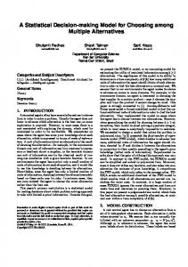
the Kyoto Protocol is x$ i , and the amount of emissions before trading is xi . We assume that each country treats the price of emissions permits parametrically. In what follows, we define the profit of each country by the surplus earned relative to the cost of achieving the assigned amount. Consider first the supplying country in Figure 1-1. The horizontal axis shows the amount of emissions of GHGs, and the vertical axis gives the marginal cost. Country i must reduce its emissions of GHGs from xi to x$ i in order to attain the target of the Kyoto Protocol. On the other hand, this country could obtain profits from the emissions permit price, p, by selling permits after reducing its GHGs by more than required in the Kyoto target. This country should consider this fact when deciding on the amount of allowable GHG emissions, xi , in that country. First, the country’s total revenue becomes p( x$ i − xi ) . Although the real cost is the area between the marginal abatement cost curve and the line segment, xi − xi , we define the profit function as xˆ

(1) π i ( xi ) = p( xˆ i − xi ) − ∫x i MAC i (t )dt , i

since we consider the profit after attaining the Kyoto target. The shadowed area in Figure 1-1 shows π i ( xi ) .

a p

0i

b

p

xi

^ x i

_ xi

0i

Figure 1-1: A Supplier

^ x i

xi

_ xi

Figure 1-2: A Demander

Figure 1: Determination of GHG Emissions Next, consider the demanding country for emissions permits. As Figure 1-2 shows, the domestic reduction cost to attain the Kyoto target is the area between the marginal abatement cost curve and the segment xi − x$ i . On the other hand, reducing emissions by xi − xi and then buying emissions permits for xi − x$ i under the price p makes the payoff

4

z

z

xi x MACi (t )dt − x i MACi (t )dt − p( xi x$ i i

− x$ i ) ,

which coincides with (1). The payoff (or profit) corresponds to the area α − β . Notice that the profits or surplus of Figures 1-1 and 1-2 are not maximized under p. In what follows, we assume that each country maximizes its surplus. Differentiating (1) with respect to xi , and then finding the maximum, xi*, we have the first-order condition (2) p = MACi ( xi*) . Furthermore, the sum of emissions for each country must equal the sum of the assigned amount for each country. Thus, we have (3)

∑ x i*

= ∑ x$ i .

Therefore, ( p*,( x1* , x2* ,L , xn* )) satisfying (2) and (3) is a competitive equilibrium. Since the

first-order condition (2) does not depend on the initial position of emissions, xi , the competitive equilibrium does not depend on the initial position or the present amount of emissions from each country. Furthermore, the competitive equilibrium is independent of the distribution of the assigned amounts for each country as long as the total sum of the assigned amounts, ∑ x$ i , which is the right-hand side of (3), is fixed. Of course, the initial position and the assigned amount do influence how much cost each country must bear. Figure 2 illustrates a competitive equilibrium in emissions trading. By superimposing the dotted vertical axis of Figure 1-2 on the dotted vertical axis of Figure 1-1, we create Figure 2 in which the vertical axis at the assigned amount corresponds to these dotted vertical axes. Country 1 reduces its GHG emissions more than the assigned amount and then sells the excess amount over the assigned amount to Country 2. On the other hand, Country 2 reduces emissions by up to x2* and then buys emissions permits from Country 1. The marginal abatement cost of each country equals to the competitive equilibrium price.

5

MAC Country 2's MAC

Country 1's MAC

2's Status Quo

Demander's Surplus

Supplier's Surplus

p* 1's Status Quo

z

x*1

x i Assigned Amount ^

_ x 1 x*2

_ x2

+

Emissions

Figure 2: Emissions Trading and the Competitive Equilibrium Consider now a social welfare problem in which the total sum of the reduction costs of all countries is minimized under the condition where the sum of emissions of all countries is equal to the sum of assigned amounts of all countries:

z

x

min ∑n1 x i MACi (t )dt subject to i x

∑ xi = ∑ x$ i ,

where x = ( x1 x2 ,L , xn ) . If x∗ = ( x1∗ , x2∗ ,L , xn∗ ) is a solution to this problem. We have

MACi ( xi* ) = MAC j ( x *j ) for all i and j . Consider next a problem where the sum of profits of all countries is maximized under the same condition. Then, the sum becomes

since

z

n xi MACi (t )dt xi

n

∑1 p( x$ i − xi ) − ∑1

n

∑ xi = ∑ x$ i , ∑1 p( x$ i − xi )

,

must be zero for any price p. Therefore, the

maximization problem of the sum of profits of all countries becomes

z

x

max − ∑n1 x i MACi (t )dt subject to i x

∑ xi = ∑ x$ i .

That is, the profit maximization problem is exactly the same as the cost minimization problem. Hence, the solution must satisfy MACi ( xi* ) = MAC j ( x *j ) for all i and j. This also implies that the sum of surpluses (or profits) of all countries is maximized as Figure 2 shows. Summarizing the above results, we have

6

Proposition 1:

(1) The price of an emissions permit is equal to the marginal abatement cost of each country ( p* = MACi ( xi*) for all i), and the sum of emissions of all countries is equal to the sum of the assigned amounts of all countries at a competitive equilibrium ( ∑ x i* = ∑ x$ i ). (2) By minimizing the sum of reduction costs of GHGs of all countries under ∑ xi = ∑ x$ i , we have MACi ( xi* ) = MAC j ( x *j ) for all i and j . (3) The sum of the reduction costs for GHGs of all countries is minimized under a competitive equilibrium. (4) The sum of surpluses of emissions trading is maximized under a competitive equilibrium. (5) The competitive equilibrium price and allocation are independent of the initial amount of GHG emissions. (6) The competitive equilibrium price and allocation are independent of the distribution of the assigned amounts as long as the sum of the assigned amounts of all countries is fixed. One of the most controversial issues in emissions trading is the so-called “hot air.” Although, for example, Russia’s assigned amount is 100% of its GHG emissions in 1990, it is estimated that the amount of emissions would be considerably less than the assigned amount after 2008 because of economic stagnation. This implies that Russia could sell emissions permits without actually reducing its GHGs domestically and that buyers of the permits could in turn increase their emissions. This amount of emissions is called “hot air.” In Figure 1, x$ i − xi is hot air as long as xi is on the left-hand side of x$ i . This hot air issue cannot be solved by using emissions trading since the competitive equilibrium allocation is determined independently of hot air as Proposition 1-(5) shows. In other words, the sum of emissions of all countries must be equal to the sum of the assigned amounts of all countries as long as we use emissions trading3. The above is a prototype of emissions trading from the viewpoint of microeconomics. We implicitly assumed that the emissions permit can be treated as a private good. However, greenhouse gases are public goods (or “bads”). Behind this approach, we further assume that we can analyze public goods as private goods by 3

See Kaino, Saijo, and Yamato (1999).

7

introducing a market for emissions permits. But the characteristics of public goods, i.e., non-rivalness and non-excludability, would not disappear with the emissions permit market. In the case of a private good, a transaction is completed if a seller delivers the good to a buyer and the buyer pays for it. On the other hand, in the case of a emissions permit, a seller must reduce GHGs at least by the amount sold and a buyer can emit GHGs by at most the amount bought in addition to the usual transaction of a private good. That is, GHG emissions and reduction must be monitored. It is claimed that actual monitoring of GHG emissions is not an easy task. Furthermore, a time lag exists between the actual emissions and the data collection of the monitoring system even when assuming that the monitoring is perfect. Between these two times, the price of an emission perimtwill fluctuate in the market. If monitoring and its verification are considerably costly, we cannot be certain that the market for emissions trading minimizes the total costs of emissions reduction. I did not describe the case when a country emits more than the assigned amount. If this were the case, the violation of the Kyoto target would benefit that country and, at the same time, reduce the country’s political trust. That is, that country should emit as much as possible to maximize its economic benefit. In other words, the above model implicitly assumes that there exists some penalty for non-compliance. That is, all countries participating in emissions trading must agree upon a penalty system including the levying of penalties and the form of the organization that levies the penalties. The penalty system necessitates additional costs. We implicitly assumed that each country treats prices parametrically. However, it is expected that the quantities demanded by Japan and the quantities supplied by Russia will be relatively large. If they exercise their market power, it is possible that the total surplus will not to be maximized. We will reconsider this problem in Section 5. The model described in this section is static. Further, we assume that each country can move on the marginal abatement cost curve freely. However, it usually takes quite a long time to replace current facilities and equipment. Moreover, the emissions reduction investment might be irreversible. That is, one can move from right to left on the marginal abatement cost curve, but not in the opposite direction. Therefore, marginal abatement costs might not be equalized.

8

3. A Social Choice Approach: Strategy-proofness Consider a mechanism that determines an allocation through gathering information that each agent has. Under this mechanism, country i reports its own marginal abatement cost curve, MACi , to an administrative institution of the United Nations. The institution recommends a competitive equilibrium allocation based upon the reported marginal abatement cost curves. Let f i ( MAC1 ,L , MACn ) be country i’s surplus accruing from the competitive equilibrium allocation when country i announces MACi , and let f = ( f 1 ,L , f n ) be a surplus function. Each country may not necessarily have an incentive to reveal its true marginal abatement cost curve, but the request that each country announces the true marginal abatement cost curve is called strategy-proofness. Let MAC i* be country i’s true marginal abatement cost curve. Then, a surplus function, f = ( f 1 ,L , f n ) , satisfies strategy-proofness if, for each country, I, it satisfies f ( MAC1 ,L , MACi − 1 , MACi∗ , MACi + 1 ,L , MACn ) (*) i for all MAC j ( j = 1,L , n) . ≥ f i ( MAC1 ,L , MACi − 1 , MACi , MACi + 1 ,L , MACn ) That is, strategy-proofness means that announcing the true marginal abatement cost curve is the dominant strategy for all i. Strategy-proofness is a strong condition since it requires that revealing the true marginal abatement cost curve is the best strategy regardless of the revelations of the others. On the other hand, it would be natural to consider that country i would change its strategy depending on the strategies of the others. This is in the spirit of the Nash equilibrium. Therefore, requiring that the revelation of the true marginal cost curve constitutes a Nash equilibrium, we have

(**)

f i ( MAC1∗ ,L , MACi∗− 1 , MACi∗ , MACi∗+ 1 ,L , MACn∗ ) ≥ f i ( MAC1∗ ,L , MACi∗− 1 , MACi , MACi∗+ 1 ,L , MACn∗ )

for all MACi

for each i. It is clear that the revelation of true marginal cost curve is a Nash equilibrium if the surplus function satisfies strategy-proofness. It may seem that condition (**) is weaker than (*), but these two conditions are in fact equivalent. Proposition 2 (Dasgupta, Hammond and Maskin, 1979): A surplus function satisfies strategy-proofness if and only if the revelation of the true marginal cost curve for each country, i, is a Nash equilibrium.

9

We will show that a surplus function does not satisfy strategy-proofness by using Proposition 2. For this purpose, it is sufficient to show that a country could benefit by announcing a false marginal abatement cost curve in a certain profile of true marginal abatement cost curves. Let the solid curves be true marginal abatement cost curves in Figure 3. Assume that country 2 reveals its true marginal abatement cost curve and country 1 announces a false marginal abatement cost curve, shown as a dotted curve. Then, the competitive equilibrium price under this condition becomes P’, which is higher than the true competitive equilibrium price. Due to this price increase, the quantity supplied would be less than that of the true competitive equilibrium. Therefore, this reduces the surplus of country 2 by α. On the other hand, country 2 increases its profit by β (= (P’-P*) x the quantity supplied) due to price increase that surpass the loss. Therefore, country 2 could benefit by not revealing its true marginal abatement cost curve. Hence, we have the following proposition. Proposition 3: A surplus function does not satisfy strategy-proofness.

MAC 1's fake MAC

b P'

Country 1's true MAC

-

Country 2's true MAC Demander's Surplus 2's Status Quo

Supplier's Surplus P*

1's Status Quo

a Assigned Amounts

Emissions

+

Figure 3. A surplus function is manipulable Johansen (1977) criticized the research program that considers resource allocation through revelation of functions. Among other things, he pointed out that public goods have never been provided through revelation of utility functions and production functions. Rather, he argued that they have been provided through political processes such as representative systems. Therefore, he indicated that research on

10

public good provision in democratic societies was necessary. . Although he expressed this opinion more than twenty years ago, very little progress has been made since then. There are many ways to evaluate Proposition 3, but we interpret this proposition as saying that the surplus function is manipulable even though transmission of marginal abatement cost curves can be done at a nominal cost through technological innovation. Additional evaluation follows in the next section. 4. Mechanism Design Approach We consider an emissions allocation problem through the revelation of marginal abatement cost curves assuming that each country does not know the marginal abatement cost curves of the other countries. However, once the emissions trading starts, each country roughly knows the marginal abatement cost curves of the other countries. As Proposition 2 indicates, there is no incentive for each country to reveal its true marginal abatement cost curve since strategy-proofness is equivalent to the condition in which the revelation of true marginal abatement cost curves is a Nash equilibrium. Therefore, apart from the revelation of curves, which requires quite a lot of information, it is worthwhile to consider an allocation problem in which the transmission of prices and quantities of emissions permits is allowed to attain the competitive equilibrium. In what follows, we show that a two-stage mechanism called the Mitani mechanism (1998) attains the competitive equilibrium allocation through information transmission of prices and quantities.4 The Mitani mechanism works if the number of participants is at least two. That is, the mechanism can overcome the problem of a small number of participants. As stated in Section 2, a country may exercise its market power when the number of countries is small. Even under this condition, the Mitani mechanism attains a competitive equilibrium allocation. Consider the Mitani mechanism with two countries, 1 and 2. In the first stage, each country announces a price simultaneously. The dotted ellipse in Figure 4 shows that country 2 does not know the price announcement of country 1. Country 2 must evaluate its transaction of emissions permits from the announced price, p1 , of country 1, and vice versa. In the second stage, knowing p1 and p2 in the first stage, country 1 announces the quantity, z,of emissions permits.

4

The Mitani mechanism is based on a compensation mechanism proposed by Varian (1994).

11

1 p

1

Stage 1

2 p2 1

Stage 2

z

Figure 4. The Mitani mechanism We define the payoff functions of countries 1 and 2 in the Mitani mechanism. For simplicity, we suppose that country 1 is a supplier of emissions permits and country 2 is a demander. Following Section 2, we define the payoff functions in comparison with the case when each country attains the assigned amount domestically. Let z be the quantity supplied by country 1. Then, the cost of reducing from x$ 1 by z is (4)

z

x$

C1 ( z) = x$ 1− z MAC1 (t )dt . 1

Since x$ 1 is the assigned amount of country 1, the cost for country 1 is a function of z. On the other hand, since the quantity supplied that is determined by country 1 becomes the quantity demanded by country 2 in the Mitani mechanism, the gross payoff of country 2 is

(5)

z

x$ + z

C2 ( z) = x$ 2 2

MAC2 ( x)dx .

Following the above, the payoff function, g i , becomes (6)

g 1 ( z , p1 , p2 ) = −C1 ( z) + p2 z − k( p1 − p2 )2 where k > 0 g 2 ( z , p 1 ) = C 2 ( z) − p 1 z

Country 1 sells its excess reduction, z, beyond its assigned amount to country 2. The price of this transaction is the price that is announced by country 2 in stage 1. The revenue from this transaction is p2 z , and the last term, k( p1 − p2 ) 2 , in g1 is a penalty term to make country 1 announce the same price announced by country 2. Country 2

12

buys z with p1 announced by country 1. Consider now how the Mitani mechanism works. First, consider the second stage. Country 1 determines z to maximize the payoff. Therefore, differentiating g 1 with respect to z and equating the result to zero, we have p2 = C1′ ( z) . That is, z is determined depending on p2 , which is determined in the first stage. Therefore, we can regard z as a function of p2 . That is, z = z( p2 ) . By substituting this expression with p2 = C1′ ( z) and differentiating with respect to p2 , we have z ′( p2 ) = 1 / C1′′ . As long as

C1′′ ≠ 0 , z ′( p2 ) is not zero. Consider now how country 1 behaves. Country 1 determines p1 to maximize the payoff. That is, by differentiating g 1 with respect to p1 , we have p1 = p2 .On the other hand, country 2 chooses p2 to maximize the payoff taking into account the behavior, z( p2 ) , of country 1. That is, by substituting z( p2 ) into g 2 and differentiating with respect to p2 , we have C2′ ⋅ z ′( p2 ) − p1 z ′( p2 ) = z ′( p2 )(C2′ − p1 ) = 0 . Since z ′( p2 ) is not zero, we have p1 = C2′ ( z) . Therefore, we have p1 = p2 = C1′ ( z) = C2′ ( z) . From (4), we have C1′ ( z) = MAC1 ( x$ 1 − z) and, from (5), we have C2′ ( z) = MAC2 ( x$ 2 + z) . That is, we have

p1 = p2 = MAC1 ( x$ 1 − z) = MAC2′ ( x$ 2 + z) . This is exactly the same expression as Proposition 1-(1). This proves that the Mitani mechanism achieves the competitive equilibrium allocation in subgame perfect equilibrium. The Mitani mechanism consists of a payoff function and a game tree as depicted in Figure 4. If marginal abatement cost curves, MAC1 and MAC2 , are given, we have a subgame perfect equilibrium ( p1 , p2 , z) . The subgame perfect equilibrium of the Mitani mechanism is unique. Let the set be N sp ( MAC1 , MAC2 ) . We write

g ⋅ N sp ( MAC1 , MAC2 ) as the evaluation of the set by g. Then, we have

(7)

f ( MAC1 , MAC2 ) = g ⋅ N sp ( MAC1 , MAC2 ) .

That is, the payoff function coincides with the surplus function under the Mitani mechanism. In other words, the Mitani mechanism implements the surplus function, f, in subgame perfect equilibrium if (7) holds for any ( MAC1 , MAC 2 ) . Let us find the set of Nash equilibria of the Mitani mechanism. Since the strategic variables of country 1 are p1 , z , by differentiating g 1 with respect to p1 and z , we have ∂g 1 ( z , p 1 , p 2 ) ∂g 1 ( z , p1 , p2 ) = −2 k( p1 − p2 ) = 0 , = −C1′ ( z) + p2 = 0 . ∂p 1 ∂z On the other hand, although the strategic variable of country 2 is p2 , this variable does not affect the payoff of country 1. That is, the payoff of country 2 does not depend on

13

the announcement of p2 . Therefore, any triple ( p1 , p2 , z) satisfying p1 = p2 = C1′ ( z) is a Nash equilibrium of the Mitani mechanism. By requiring C1′ ( z) = C2′ ( z) in addition to the condition, we obtain a subgame perfect equilibrium. That is, the set of subgame perfect equilibria is a proper subset of the set of the Nash equilibria. Therefore, the Mitani mechanism cannot implement the surplus function under a Nash equilibrium. We implicitly assume that there must exist a central body that determines who the participants in the mechanism are, collects information, and conducts resource allocation based upon the information that the mechanism requires. In particular, participants must be all countries in the case of global warming, but some country may not want to participate in and benefit from the reduction of greenhouse gases by other countries.5 As for the collection of information, a participant may not transmit the information required by the mechanism to the body even though the participant agrees to participate in the mechanism. When participants announce their willingness to participate in the mechanism, the central body must have some power to collect information about the strategies of the participants under the framework of social choice or the mechanism design approach. These two approaches implicitly assume that there exists a body with central power.6 We consider the validity of the Mitani mechanism in the following section. 5. An Experimental Approach Even though we have succeeded in constructing a theoretical mechanism, we are not certain that it works. Using it in the real world would be risky since the economic damage from a possible failure would be unbearable. Furthermore, we would not be able to determine whether the failure of the mechanism is due to some flaw in the mechanism or some other outside factors. An alternative way to assess the performance of the mechanism is a laboratory experiment. We construct an experimental model out of the theoretical model. Usually, theory does not indicate the number of agents in the model, the exact shape of the functions used in the model, and what types of information each agent has. In an experimental model, these variables must be specified. Depending on how we assign these parameters, we have many possible cases. Our methodology calls for recruiting subjects and paying them contingent upon their performance. By conducting several experiments and then comparing the results, we can understand the effects of these parameters. We utilize two experiments conducted by Hizen and Saijo (2001) and Hizen, Kusakawa, Niizawa, and Saijo (2000), whose models of the experiments are based upon 5 6

Saijo andYamato (1999) consider an equilibrium when participation is a strategic variable. The same problem exists under social choice approach.

14

the microeconomic approach in Section 2. Section 6 describes an experiment that Mitani, Saijo, and Hamaguchi (1998) designed to assess the performance of the Mitani mechanism. The main question of the experiments by Hizen and Saijo (2001) and Hizen. –Kusakawa, Niizawa, and Saijo (2000) is whether the total surplus is maximized under emissions trading. The emissions trading model in Section 2 implicitly assumes that transactions are conducted under a competitive equilibrium, but the surplus of each country can be different from the surplus at the competitive equilibrium depending on the methods of transaction. In order to avoid problems due to non-compliance to the assigned amounts, Hizen and Saijo (2001) designed their experiment so that the assigned amounts are always satisfied in the course of transactions and compared two trading institutions, namely, the double auction and bilateral trading. On the other hand, Hizen, Kusakawa, Niizawa, and Saijo (2000) explicitly incorporated non-compliance and decision making on domestic reductions into their experiment. Prior to Hizen and Saijo (2001) and Hizen, Kusakawa, Niizawa, andSaijo (2000), Bohm (1997) conducted an important emissions trading experiment. He recruited bureaucrats from the Ministry of Energy and specialists from Finland, Denmark, Norway, and Sweden, and then conducted an emissions trading experiment in which each country could buy and sell emissions permits under bilateral trading. The subjects knew the marginal abatement cost curves of other countries, but not the true curves. It took four days to complete a single period by using facsimile communication to exchange information on prices and quantities. The average transaction price was very close to the competitive equilibrium price and the efficiency wais 97%, which is quite high. Many economists have expressed the opinion that it is difficult to attain efficiency if a trading agent is a country as a unit, but Bohm has shown that it is possible to attain high efficiency when countries are the players. I start with an overview of the common features of the experiments of Hizen and Saijo (2001) and Hizen, Kusakawa, Niizawa, and Saijo (2000). Six subjects participated in a session. The subjects were supposed to represent Russia, Ukraine, the US., Poland, the EU, and Japan. In the experiments, no country names were given to subjects. Subjects must have assumed that they were engaged in transactions of an abstract commodity. Figure 5 shows the marginal abatement cost curves used in the experiments. The origin is the assigned amount for each country. In the experiments on information disclosure on the marginal abatement cost curves, every subject had Figure 5 at hand. On the other hand, in the experiments on information concealment, each subject only knew his/her marginal abatement cost curve.

15

1-Russia 2-Ukraine 3-USA 4-Poland 5-EU 6-Japan

2

1

3 240

215

250

250

240

(-45)

6

5

4

(-15)

(-27)

220

216

(-80)

(-50)

250

(-5)

210

200

(-10)

180

(-35)

200 (5)

(-22)

165

166

(-73)

(-20)

120

130 (10)

90 (-55) (-20)

70

(-10)

100

90

100 80

(20)

(-5)

88 (35)

(25)

60

40 50

(-32)

122 (23) (25) 118

(-17)

(-30)

60

150

(15)

142

150 120

118

(-65)

170

162

(-40)

190

(-10)

30

20 (10)

(50)

(40)

(55)

40 20 (33)

-80

-70

-60

-50

-40

-30

-20

-10

0

10

15

20

30

45 50

60

Figure 5. Marginal Abatement Cost Curves used by Hizen and Saijo and Hizen, Kusakawa, Niizawa, and Saijo Two trading methods were used in the experiments. The first one was bilateral trading. Two out of six subjects made a pair and then negotiated the price and quantity of the emissions permits. The maximum number of pairs was three because of the limit of six subjects. During the negotiation, subjects were not allowed voice communication, but communicated by means of writing the numerical values of price and quantity. Written responses of “yes” and “no” were allowed. Once a pair reached an agreement, the pair was supposed to inform the experimenter. In the case of disclosure of information of the contract, the experimenter wrote the information on the blackboard and announced it to every subject. The pair again returned to the floor to seek other contracts. This procedure lasted up to 60 minutes. The second method was a double auction. Six subjects were placed together. Subjects who wanted to sell announced the price and quantity, and subjects who wanted to buy made similar announcements. Table 1 shows an example of the auction. A subject who wanted to announce price and quantity raised his/her hand. The experimenter called on the subject (subject 3 in the example since he/she was the first person to raise his/her hand). The subject then called out that he/she wants to buy 20 units at $56 for each unit, and the experimenter wrote the information on the blackboard. Right after this announcement, another subject (subject 6 in the example)

16

announced his/her willingness to sell 15 units at $104 for each unit. Since the spread of the price difference was quite high, subject 1 announced his /her willingness to buy 13 units at $86. Then, subject 4 announced his willingness to sell 20 units at $92. Right after this announcement, subject 2 accepted the offer from subject 4. The maximum number of units was 20. This process then continued. An important feature of the double auction is that each subject receives the information of the announcements simultaneously. In contrast, in the case of bilateral trading only a pair knows the information as long as the experimenter does not reveal it. Buyers' Bids

Sellers' Asks

(3) $56, 20 units

(6) $104, 15 units

(1) $86, 13 units

(4) $92, 20 units

(2) grabs (4)' ask

: :

: :

Table 1. An Example of the Double Auction Next, we consider the Hizen and Saijo’s (2001) experiment. In order to avoid the non-compliance problem, the starting point of the transaction for each subject was the assigned amount (see squares at the vertical axis going through the origin in Figure 6). When this is the case, the target of the Kyoto Protocol is automatically satisfied at any point in the transaction. As Propositions 1-(5) and 1-(6) show, the competitive equilibrium in Figure 2 coincides with the one in Figure 6. The squares in Figure 6 show the initial points of transactions. Furthermore, Hizen and Saijo assumed that subjects can move on the marginal cost curves freely in order to avoid investment irreversibility in which a subject cannot go back to the left once he/she decides to choose a point on the curve.

17

Country B's Country A's MAC MAC

MAC P*: competitive equilibrium price B's Status Quo Demander's Surplus

Supplier's Surplus

P* A's Status Quo

Assigned Amounts

+

Amount of Emissions

Figure 6. Initial Points of Transactions and Emissions Trading in Hizen and –Saijo’s Experiment Subjects were paid in proportion to their performance in the experiment. In the Hizen and –Saijo’s (2001) experiment, subjects were instructed about how they could obtain monetary reward by showing them a sample graph such as Figure 7. The point of departure was the assigned amount in Figure 6 that corresponded to “your position” in Figure 7. Consider, as an example, the upper central graph in Figure 6. The horizontal line shows the price line. Since the marginal abatement cost is higher than the emissions permit price, the subject can benefit by buying a permit. If he/she succeeds in buying the permit up to the intersection point between the marginal cost curve and the price line, he/she could obtain the benefit corresponding to the benefit area in Figure 7. After the transaction, the position of the subject moves. A new transaction starts from this new position. Figure 7 shows all the possible cases.

18

Price

Price

Price Benefit

B

B

A

Paying Price

A

B A

Benefit

Buy!

Your Position

Sell!

Your Position

No Transaction Price

Buying Price

Your Position Price

Price Profit

Buying Price

Paying Price Profit

Buy!

Your Position

No Transaction

Sell!

Your Position

Your Position

Figure 7. Benefits and Profits of Subjects Consider next the controls in Hizen and Saijo’s experiment. In the bilateral trading setting, two controls were used. The first was the marginal cost curve information depending on if the subjects knew all the marginal cost curves. The second was the contract information depending on the concealment or disclosure of the contracted price. Although the assumption that each country knows all the marginal abatement cost curves is unrealistic, we employed it because Bohm (1997) observed high efficiency under the condition that every country knows the curves fairly well. By comparing the results with full information of marginal abatement cost curves to the ones with only private marginal abatement cost information, we can measure the effect of the information disclosure. In the case of the double auction, only the marginal abatement cost information control is employed since the contract information is available to every country. For each cell in Table 2, at least two sessions were conducted with different sets of subjects.

19

Marginal Abatement Cost Curve Information Disclosure (O) Closure (X)

Bilateral Contract Trading Information

Disclosure (O) Closure (O)

OO OX XO XX Disclosure (O) Closure (X)

O

Double Auction

X

Table 2. Controls in Hizen and –Saijo’s Experiment Consider Hizen and Saijo’s (2001) experimental results from the viewpoint of efficiency. As Proposition 1-(4) shows, the total surplus is maximized at the competitive equilibrium. That is, the total surplus accruing from any trading rule cannot exceed the total surplus of the competitive equilibrium. Therefore, define a measure of efficiency as follows: The sum of the surplus of all subjects/The total surplus of the competitive equilibrium Therefore, the maximum efficiency is one or 100%. In the Hizen and Saijo’s (2001) experiment, the competitive equilibrium price is between 118 and 120. Therefore, we take the average 119 as the competitive equilibrium price. When the transaction is conducted under this price, the total sum of the surplus is 6990. The first row in Table 3 shows the trading rule, and the second shows the names of the sessions. For example, “OX2” under bilateral trading indicates the disclosure of contract prices, the closure of marginal cost curve information, and the second session of this condition. That is, “O” indicates “disclosure” and “X” indicates “concealment.” The first digit indicates the contract information; the second one indicates the marginal cost curve information; and the last digit indicates the session number. Since the contract information is disclosed in the double auction, “X1” indicates the concealment of the marginal cost curve information and the first session of this control. The number in the leftmost column indicates the subject number; the number in parentheses indicates the surplus obtained by the subject at the competitive equilibrium. In each cell, the upper number is the surplus that the subject actually obtained in the experiment, while the lower number is the individual efficiency. For example, the individual efficiency of subject 1 is 0.732, which is obtained by the ratio of the surplus at the competitive equilibrium (2555) to the actual surplus (1870). The individual efficiency is different from the session efficiency.

20

The former may exceed one since the distribution of total surplus depends on how the transactions are carried out although the total sum of the surplus cannot exceed 6990. Some subjects might have low efficiency since they sell their emissions permits for less than the competitive price. On the other hand, some might attain high efficiency by buying permits at low prices. In the experiment, the maximum monetary reward was 7600 yen, the minimum 2000 yen, and the average 3459 yen.

Bilateral Trading OO1 OO2 OX1

OX2

XO1

XO2

XX1

XX2

1710 0.669 1665 1.291 372 0.610 530 1.359 755 1.218 1844 1.209 6876 0.984

1510 0.591 1320 1.023 1846 3.026 500 1.282 -150 -0.242 1400 0.918 6426 0.919

1100 0.431 940 0.729 615 1.008 555 1.423 1080 1.742 2700 1.770 6990 1

1460 0.571 1536 1.191 583 0.956 910 2.333 81 0.131 2390 1.567 6960 0.996

1600 0.626 2370 1.837 550 0.902 500 1.282 150 0.242 1800 1.180 6970 0.997

Double Auction O1 O2

O3

X1

X2

1981 0.775 520 0.403 1144 1.875 230 0.590 1380 2.226 1695 1.111 6950 0.994

2260 0.885 1770 1.372 681 1.116 209 0.536 700 1.129 1350 0.885 6970 0.997

2865 1.121 1120 0.868 1270 2.082 355 0.910 0 0.000 1360 0.892 6970 0.997

Subject No.

1 (2555) (Russia) 2 (1290) (Ukraine) 3 (610) (U.S.A.) 4 (390) (Poland) 5 (620) (EU) 6 (1525) (Japan)

1420 0.556 1140 0.884 685 1.123 520 1.333 800 1.290 2425 1.590 Sum (6990) 6990 1

1870 0.732 914 0.709 683 1.120 570 1.462 1105 1.782 1800 1.180 6942 0.993

960 0.376 360 0.279 2060 3.377 850 2.179 1300 2.097 1450 0.951 6980 0.999

2410 0.943 1320 1.023 850 1.393 200 0.513 750 1.210 1430 0.938 6960 0.996

2410 0.943 1320 1.023 865 1.418 350 0.897 500 0.806 1515 0.993 6960 0.996

Table 3. Efficiencies in Hizen and –Saijo’s experiment As Table 3 shows, the efficiency of each session was quite high except for the “XO1” session. Subject 5 in this session traded even though he/she suffered considerable losses. On the other hand, individual efficiencies varied even in subjects who had the same i.d. number. In bilateral trading, Russia’s efficiencies were lower than those of the competitive equilibrium, and Poland’s efficiencies were higher than those of the competitive equilibrium. We cannot say that the efficiencies of the other countries were statistically different from one another. On the other hand, under the double auction, the efficiencies of the US were higher than those of the competitive equilibrium, Poland’ efficiencies were higher than those of thecompetitive equilibrium, and the efficiencies of the others were statistically close to one.

Consider now the efficiency dynamics over time. Under bilateral trading, the efficiencies of all sessions, except for session XX2, exceeded 80%, and the efficiencies immediately after 25 minutes exceeded 90% in six out of eight sessions. The efficiencies increased monotonically, but the efficiency of session OX2 fluctuated since one subject

21

bought permits at a loss and then sold some of them at a relatively high price. Under the double auction, the efficiencies of all sessions, except for session X2, exceeded 70% immediately after 17 minutes and exceeded 90% after 44 minutes. They increased monotonically, but we observed a decrease in the X sessions after achieving 100%. For example, in session X2 ,one subject sold permits at a loss while expecting to buy them at a relatively low price, but could not. Such losses were not observed when the marginal cost curve information was disclosed. These results led to the following observation: Observation 1.

(1) The efficiency of bilateral trading is almost one, regardless of concealment or disclosure of price and marginal abatement cost information. (2) Russia's efficiency is low; Poland's efficiency is high; and the efficiency of the other countries is close to one. (3) The efficiency of allocation in 6 of 8 sessions was more than 90% after 25 minutes. We employed the following method to check the convergence of the transaction prices. If the variance of the last three transactions was significantly smaller than that of the first three transactions, we said that the transaction price sequence converged. We also regarded the average of the prices of the last three transactions as the converged price if the sequence converged. This resulted in the following observation. Observation 2 (Bilateral Trading).

(1) The contracted average prices in the "XX" sessions (concealment of prices and concealment of marginal abatement cost curves) were roughly equal to the competitive equilibrium price, but the variances in the contracted prices in the "XX" sessions were larger than those in the rest of the sessions. (2) The contracted average prices cannot be said to equal the competitive equilibrium price in sessions other than the "XX" sessions. (3) The average price of the last three contracts is not equal to the competitive equilibrium price in any session.

22

(4) Convergence of the contracted prices is found in five of eight sessions, but no information disclosure effect on convergence is observed. Under bilateral trading, the price that a pair agrees on is determined by the negotiation. Even when the transaction prices are open to every subject, a proposal such as "let us agree upon the price that is used by other subjects" can be rejected by the other subject. In other words, negotiation power is an important factor, and, hence, it would be difficult to say that the sequence converged to the competitive equilibrium price. On the other hand, in the double auction, the price sequence converged to the competitive equilibrium price, leading to the following observation: Observation 3 (Double Auction).

(1) The contracted price sequence converged to the competitive equilibrium price regardless of concealment or disclosure of the price and marginal abatement cost information. (2) The average price in sessions O1, O2 and X1 were close to the competitive equilibrium price.. (3) The average price of the last three transactions in sessions O1, X1 and X2 were close to the competitive equilibrium price.

In order to understand the effect of the disclosure of transaction information, we should compare the results in sessions OO and XO with sessions OX and XX, respectively. However, since we found that the variance in the contracted prices in session OX1 is significantly different from that in session OX2, we excluded them in the comparison. Instead, we compared sessions OO and XO, where no difference in variance was observed. Similarly, the effect of the disclosure of the marginal abatement cost curves can be seen by comparing sessions XO and XX. We found that the variance in sessions XO is statistically smaller than that in sessions XX. Summarizing the above results, we make the following observation: Observation 4 (Bilateral Trading).

(1) Assuming that the marginal abatement cost curves are public information, the disclosure of contracted prices does not have any impact on the variance of in contracted prices. (2) Under the concealment of contracted prices, the disclosure of marginal abatement cost curves reduces the variance of contracted prices.

23

Let us now consider the effect of disclosure of the marginal cost curve information. The variance in the O sessions is smaller than that in the X sessions. Russia, Ukraine, and Poland are sellers and the US., EU, and Japan are buyers at the competitive equilibrium. We observed that this happened in the O sessions, but there was at least one subject who bought and sold permits. The numbers of transactions were 9, 8 and 7 in sessions O1, O2, and O3, respectively, and they were 11 and 12 in sessions X1 and X2, respectively. Summarizing the above findings, we make the following observation: Observation 5 (Double Auction). The disclosure of marginal abatement cost curves:

(1) reduces the variance of contracted prices; (2) makes Russia, Ukraine and Poland only sell, and the US, EU and Japan only buy; (3) reduces the number of trades. Aside from the efficiencies, we can also see how the marginal abatement costs changed over time. Due to the step-function nature of our marginal abatement cost curve, we must be careful when evaluating marginal costs. For example, the marginal abatement cost of Russia in session "OO1" was 90 after 25 minutes. In the raw data, we find that Russia sold exactly 55 units of emissions allowances in 25 minutes. Therefore, if the subject wanted to sell one more unit, its marginal abatement cost would have been 120 (see Figure 5). Taking account of this fact, we make the following observation: Observation 6.

(1) In bilateral trading, except for the EU subject in session "XO1," the marginal abatement costs of all subjects approach the competitive equilibrium price, but the contracted prices do not. (2) The Marginal abatement costs of all subjects approach the competitive equilibrium price. In our double auction experiment, marginal abatement costs converged less rapidly than in the bilateral trading setting. We conjecture that this arises because at most one pair in the double auction can trade at the same time while at most three pairs can do so under bilateral trading. In order to understand how much market power a country has, we need an

24

aggregate excess demand curve of all the subjects regarding the marginal abatement cost curves as the excess demand curves for emissions allowances. In our design, the competitive equilibrium price range is from 118 to 120, while the excess demand for permits is zero under this price range. Each country might be able to change the equilibrium price by increasing (or decreasing) the quantity supplied (or demanded). If so, and the surplus of this country under the new equilibrium price is greater than the surplus under the true equilibrium price. Then we say that the country has market power. After careful examination, we find that the only country that has market power in our design is the US. Table 3 shows that the benefits of the US were more than three times larger than the benefit at the competitive equilibrium in two out of eight sessions under bilateral trading. A statistical test shows that the US did not exercise its market power in any session. Most probably, the subjects could not exploit the marginal abatement cost curve information to use their market power. Under double auction, the individual efficiency of the US is statistically greater than one. It is remarkable to find that high efficiency was observed even when there existed a subject who had market power. What would happen if subjects could easily find out that they have some market power and the transaction is done by double auction? Bohm (2000) found that the efficiency in this setting is still high, but the distribution of the surplus is distorted. That is, it is often said that the efficiency of the market would be damaged when there are countries that have market power, but this is not confirmed in laboratory experiments. It seems that the double auction and the typical explanation of a monopoly are totally different from each other. In a textbook theory of monopoly, a monopolist offers a price to every buyer, and a buyer must accept or reject the price. The second point is that a country that is supposed to be a seller under the competitive equilibrium price would be a buyer if the price of permits were considerably low. Consider the policy implications of Hizen and –Saijo’s experiment. If the main target of a policy maker is efficiency in achieving the Kyoto target, both bilateral trading and the double auction can attain this goal. If the policy maker’s target is to achieve equity so that the same permits must be traded at the same price, the double auction is better than bilateral trading. If market power is not exercised, then it seems that bilateral trading is better than the double auction. If the policy maker believes that the information transaction takes a considerable amount of resources, then the double auction is better than bilateral trading. Hizen, Kusakawa, Niizawa and Saijo (2000) focus on two assumptions that are employed by Hizen and Saijo (2001). The first is that the starting point of the transaction

25

in Hizen and Saijo is the assigned amount of the Kyoto target. The second is that a country can move on the marginal abatement cost curve freely. This assumption is made to avoid the non-compliance problem. In Hizen, Kusakawa, Niizawa and –Saijo’s (2000) experiment, the starting point of the transaction becomes more realistic as a circle on the marginal cost curve shown in Figure 5. Furthermore, they impose two restrictions on the movement on the marginal cost curve. A country can move on it from right to left, but not in the opposite direction. Once a country spends resources for abatement, it cannot reduce its marginal abatement costs through increased emissions. This corresponds to investment irreversibility. Once an agent invests some resources, the agent cannot go back to the original position. The second restriction is a condition on the decision making on domestic abatement. During 60 minutes of transactions, a country must decide on its domestic abatement decision within half an hour. This reflects that it takes a considerable amount of time to reduce emissions after the decision is made. On the other hand, emissions trading can be conducted any time during the 60 minutes. Under these new conditions, a country might not be able to attain the assigned amount of emissions. If this is the case, then the country must pay a penalty of $300 per unit. This is considerably high since the competitive equilibrium price range is from $118 to 120. In Hizen, Kusakawa, Niizawa, and –Saijo’s (2000) experiment, the marginal abatement cost curves are private information. The trading methods are bilateral trading and double auction. In bilateral trading, the control is the disclosure of contract price information (O) or the concealment of this information (X). In the double auction, this information is automatically revealed to everyone. The rest of the design is the same as in Hizen-Saijo's experiment. Table 4 is similar to Table 3. Let us explain the two numbers under the name of each country. The US has (55, 50), for example, indicating that the initial point is 55 and the competitive equilibrium point after the transaction is 50 (Figure 5). Now, consider the two numbers in the data. The numbers for the US in session O4 in bilateral trading is (23,-2). The first number shows that the US conducted 32 (=55-23) units of domestic reduction, which resulted in 23 units on the horizontal axis by moving the marginal abatement cost curve. In order to comply with the Kyoto target, the US must buy at least 23 units of emissions permits, but since the US bought 25 units, this resulted in -2 on the horizontal axis. That is, the US achieved 2 units of over-compliance. We have two kinds of efficiency. The first is the actual efficiency attained. That is, actual efficiency measures the actual surplus attained in each experiment after assigning a zero value to units of over-compliance and $300 for each unit of

26

non-compliance as $300. This is shown in the bottom row of Table 5. For example, the actual surplus of session O4 is 5736 and its efficiency is 0.821. The second kind of efficiency is the modified efficiency that reevaluates units of over-compliance and units of non-compliance by using the concept of opportunity costs. Details are given in Hizen, Kusakawa, Niizawa, and Saijo (2000). This is shown underneath the box in Table 5. For example, the modified surplus of session O4 is 6596 and its modified efficiency is 0.944. The average efficiency (the modified efficiency) in the X sessions is 0.605 (0.811); in the O sessions it is 0.502 (0.807); and in the D sessions it is 0.634 (0.873). Bilateral Trading X1 X2 Subject No. 1 (2555) (Russia) (-32)(-55,0) 2 (1290) (Ukraine) (-10)(-30,0) 3 (610) (U.S.A.) (55)(50,0) 4 (390) (Poland) (-5)(-10,0) 5 (620) (EU) (25)(20,0) 6 (1525) (Japan) (40)(25,0) Sum (6990)

1535 0.601 -40, 0 766 0.594 -28, 0 1046 1.715 23, 0 240 0.615 -5, 0 -650 -1.048 5, -5 2175 1.426 35, 0 5112 0.731 5612 0.803

X3

1600 620 0.626 0.243 -32, 0 -65, -22 1175 1820 0.911 1.411 -20, 0 -30, 0 220 556 0.361 0.911 23, 0 30, 3 100 20 0.256 0.051 -10, 0 -17, 0 375 850 0.605 1.371 10, 0 25, 0 2130 -3100 1.397 -2.033 25, 0 15, -25 5600 766 0.801 0.110 6230 4136 0.891 0.592

O1

O2

O3

O4

Double Auction D1 D2

656 1415 0.257 0.554 -42, 0 -55, -3 700 -565 0.543 -0.438 -20, 0 -20, -15 1416 -4130 2.321 -6.770 23, 0 -20, -30 94 77 0.241 0.197 -10, 0 -10, 0 850 1002 1.371 1.616 20, 0 20, 0 1710 1931 0.245 1.266 35, 0 35, 6 5426 -270 0.776 -0.039 6686 3140 0.957 0.449

384 0.150 -52, 0 2625 2.035 -20, 0 -4094 -6.711 50, 23 500 1.282 -10, 0 975 1.573 20, 0 2040 1.338 25, 0 2430 0.348 6680 0.956

1825 0.714 -33, 0 1285 0.996 -25, 0 481 0.789 23, 0 300 0.769 -13, 0 630 1.016 20, 0 1625 1.066 25, 0 6146 0.879

1465 0.573 -52, 0 2200 1.705 -20, 0 316 0.518 23, -2 450 1.154 -10, 0 965 1.556 20, -2 340 0.223 30, -5 5736 0.821 6596 0.944

1425 2435 0.558 0.953 -55, 0 -65, 0 1195 -30 0.926 -0.023 -30, 0 -30, -27 890 641 1.459 1.051 40, 0 23, 0 165 275 0.423 0.705 -10, 0 -10, 0 760 -900 1.226 -1.452 20, 0 10, -10 2515 25 1.649 0.016 35, 0 25, -10 6950 2446 0.994 0.350 5856 0.838

X4

D3

D4

1360 2060 0.532 0.806 -44, 0 -60, 0 850 -1925 0.659 -1.492 -20, 0 -30, -37 769 -404 1.261 -0.662 23, 0 23, 0 375 763 0.962 1.956 -11, 0 -17, 0 770 682 1.242 1.100 20, 0 20, 0 1822 1200 1.195 0.787 25, -5 25 , 0 5946 2376 0.851 0.340 6426 5186 0.919 0.742

Table 5. Efficiencies in the Hizen, Kusakawa, Niizawa, and –Saijo’s (2000) experiment After a careful look at Table 5, we make the following observation. Observation 7.

(1) Russia's domestic reductions were not enough in bilateral trading, but they were close to the domestic reduction at competitive equilibrium in the double auction. (2) The US conducted excessive domestic reductions in all sessions. (3) In bilateral trading, nine cases of over-compliance and three cases of non-compliance out of 48 cases were observed. On the hand, in the double auction, five cases of over-compliance and no case

27

of non-compliance out of 24 cases were observed. In order to understand the nature of investment irreversibility, Hizen, Kusakawa, Niizawa, and Saijo (2000) introduced a point equilibrium. In Figure 8, the competitive equilibrium price is P*. If country 2 continues to climb the marginal abatement cost curve, the price that equates the quantity demanded and the quantity supplied should go down and it should be P**. We call this "should be" price the point equilibrium price. Even though the point equilibrium price is P**, countries might have been trading permits at a higher price than P*.

MAC

Country 1

Country 1's MAC

P*

Position after Domestic Reduction

MAC

Country 2's MAC



Position after Domestic Reduction

P*

P**

01

Country 2

Emissions

Assigned Amount

02

Assigned Amount

Emissions

Figure 8. Point Equilibrium In each session, we have two pieces of price sequence data. One is the actual price, and the other is the point equilibrium price. With the help of the point equilibrium price, we found two types of price dynamics. The first is the early point equilibrium price decrease case (or type 1), and the second is the constant point equilibrium price case (or type 2). We observed five sessions of type 1 and seven sessions of type 2 out of 12 sessions. Figure 9 shows two graphs of type 1 and type 2 price dynamics. The top picture shows a typical case of type 1 and the bottom a typical case of type 2. The horizontal axis indicates minutes, and the vertical axis prices. The horizontal line indicates the competitive equilibrium price, and the dark step lines indicate the point equilibrium prices. A box indicates a transaction. The left-hand side is the seller's name;the right hand side is the buyer's name; and the bottom number indicates the number of units in the transaction. A diamond indicates the domestic reduction. Consider the top graph that is for session D2. Up until 15 minutes, we observe many 28

diamonds that indicate domestic reduction. This reduction seems to come from fear of non-compliance of demanders. This causes the the transaction price to be higher. Even after the point equilibrium price decreased after 10 minutes, the actual transaction prices were considerably higher than point equilibrium prices. That is, high price inertia was observed. After half an hour, no domestic reduction was possible and the point equilibrium becomes zero. We measured the area between the competitive equilibrium price line and the point equilibrium price curve up to half an hour as the discrepancy area. In the case of the bottom graph, the starting price was relatively low. Due to this low price, supply countries did not conduct enough domestic reduction. After 10 minutes and until 30 minutes, the demand countries conducted considerable domestic reduction. In this case, the point equilibrium price curve coincided with the competitive equilibrium price line. That is, the discrepancy area was zero.

280

Price

D2

260

R: Russia P: Poland U: Ukraine E: EU J: Japan A: USA

240 220

A 10 U sold 10 units to A

J

U

5 J conducted 5 units of domestic reduction

200 180 160 140 120

R

100

A

A 30 5 P

80

P 5

A J U JR J 10 R E 10 15 20 E 10 A J R UA A 2 10 10 10 25 R E 5 J 5 23

5

A

Discrepancy Area

UP 2

R 5

10

60

The Early Price Decrease Case Permit surplus: 47

40 20

R

0

U 5

0

5

10

15

20

25

30 35 Minutes

29

40

45

50

55

60

280

Price

260

D1

R: Russia P: Poland U: Ukraine E: EU J: Japan A: USA

240 220 200

J

A 10 U sold 10 units to A U

5 J conducted 5 units of domestic reduction

180 160 140 R J P A E AJ A 10 U J 5 10 5R E R EP J A 10 15 5 5 5 J R R E 10 R J R 5 3 10 5 P 20 U 5

120 100 80 60

R

5

AU

5

U A 10 A 10 A 10 U

J

EU 5

E 5

The Constant Price Case Permit surplus: 0

10

40 20 0 0

5

10

15

20

25

30 35 Minutes

40

45

50

55

60

Figure 9. Price Dynamics of Hizen, Kusakawa, Niizawa, and –Saijo’s experiment Figure 10 illustrates the relationship between the modified efficiency and the discrepancy area. By cluster analysis, we have found two groups, type 1 and type 2. Although the number of sessions was quite small, within the same type, it seems that efficiencies of the double auction were higher than those of bilateral trading and that information disclosure increased the efficiency. Summarizing these findings, we make the following observation: Observation 8.

(1) Two types, i.e., the early point equilibrium price decrease case and the constant point equilibrium price case were observed. (2) Excessive domestic reduction was observed in both types. (3) In both types, efficiencies in the double auction were higher than those in bilateral trading. (4) In type 1, we observed high price inertia and a sudden price drop. (5) In type 2, insufficient domestic reduction from the supply countries caused excessive domestic

30

reduction from the demand-countries. The sudden price drop observed in Observation 8-(4) would be overcome by banking, which is allowed in the Kyoto Protocol. Muller-Mestelman (1998) found that banking of permits had some power to stabilize the price sequence. Furthermore, under either trading rule, early domestic reduction resulted in type 1 and caused a efficiency lower than that of type 2. It seems that haste makes waste. (1) The Early Point Equilibrium Price Decrease Case

1600 44.9%

Discrepancy Area

1400

83.8%

O1

D2

(-3.9%)

1200

(35.0%)

D3

1000

(85.1%) 74.2%

800

59.2%

X3

600

D4

(34.0%)

94.4%

(11.0%)

O4

400 200 0 0.00

91.9%

(82.1%) 87.9% 95.7% (2) The Constant Point Equilibrium Price Case

0.20

0.40

O3

80.3%

X1

0.60

Modified Efficiency

(73.1%) 0.80

89.1%

X2

(80.1%)

X4

(77.6%) 99.4% 1.00 D1 95.6%

O2

(34.8%)

Figure 10. The Relationship between Modified Efficiency and the Discrepancy Area

31

6. Experimental Approach (2) This section describes the experimental results of Mitani, Saijo, and Hamaguchi (1998) who studied the Mitani mechanism. In their experiment, they specify cost functions, C1 (z ) and C2 (z ) , as follows. C1 ( z) = 37.5 + 0.5(5 + z)2 , C2 ( z) = 15 z − 0.75 z 2 .

Furthermore, the penalty function of country 1 is specified by

d ( p1 , p 2 ) =

RS 0 if p1 = p2 , where K > 0 . TK if p1 ≠ p2

Thus, if countries 1 and 2 announce the same price, then the penalty is zero; if not, then the fixed amount of penalty is imposed on country 1. Therefore, the payoff functions of the mechanism become g 1 ( z , p 1 , p 2 ) = −C 1 ( z ) + p 2 z − d ( p 1 , p 2 ) . g 2 ( z , p 1 ) = C 2 ( z) − p 1 z Even with modification of the Mitani mechanism, the subgame perfect equilibrium would not be changed. Applying the condition of subgame perfect equilibrium to the Mitani mechanism, p1 = p2 = C1′ ( z) = C2′ ( z) , we have C1′ = 5 + z , C2′ = 15 − 1.5 z , and hence z = 4 . That is, p1 = p2 = 9 . The experimental test of the Mitani mechanism is designed so that each agent is supposed to minimize the cost. Therefore, by putting a minus sign in the payoff of country 1, we have The total cost of country 1 = 37.5+0.5 × (5+the units of transaction)2 - (the price that country 2 chose) x (the units of transaction) + the charge, where the charge term is d( p1 , p2 ) . We regard the payoff of country 2 as the surplus accruing from buying emissions permits from x∗2 to the assigned amount ( x$ 2 ) as shown in Figure 2. On the other hand, in the Mitani, Saijo, and Hamaguchi’s experiment, the sum of the cost-reducing emissions from x2 to x∗2 and the payment p * ( x∗2 − x$ 2 ) for

32

emissions are the total cost. This does not change the subgame perfect equilibrium of the Mitani mechanism since it merely changes the starting point for either the payoff or cost. When x2 = 10 , C2 (10) − C2 ( z) = 75 − 15 z + 0.75 z 2 = 0.75(10 − z)2 is the cost of reducing the amount of emissions from x2 to x∗2 . That is, The total cost of country 2 = 0.75 × (10-the units of transaction)2 +(the price that country 1 chose) ×(the units of transaction). When no transaction occurs, the total cost of country 1 is 37.5+0.5×52, which equals 50 and the total cost of country 2 is 0.75×102, which is 75, where the charge term is zero. Let us review the experiment. Two sessions were conducted, one for K = 10 and the other for K = 50 . Each session included 20 subjects who gathered in a classroom and divided into 10 pairs. Each subject could not identify the other dyad member. During the experiment, "emissions trading" were not used. Country 1 in the above corresponded to subject A, and country 2 to subject B. The experimenter allotted 5 units of production to Subject A and 10 units to subject B. Then the transaction of allotted units of production was conducted by a certain rule (i.e., the Mitani mechanism). The allotted amounts corresponded to the reduction amounts in theory. In order to prepare an environment in which one subject (A) knew the production cost structure of the other subject (B), we explained the production cost to both subjects, and then conducted four practice rounds. Two were for subject A and two for subject B. Right before the real experiment, we announced who was subject A and who was B. Once the role of the subjects was determined, it remained fixed across 20 rounds. Table 6 displays the total cost tables for subject A. The upper table is the payoff table for subject A. The payoff for subject A is determined by pB , announced by subject B and the amount of transaction, z, by subject A without considering the charge term. If the prices announced by both subjects were different, subject A paid the charge. Subject A could also see the payoff table for subject B, which is shown in the bottom table in Table 6. The payoff for subject B is determined by p A and z is announced by subject A. That is, subject B cannot change his or her own payoff by changing pB . We will find the subgame perfect equilibrium through Table 6. Subject A first solves the optimization problem in stage 2 and then chooses a z that minimizes the total cost of subject A depending on the announcement of pB by subject B. This is z = z( pB ) . For example, if pB = 6 , then z = 1 . The diagonal from the upper left to the bottom right corresponds to z = z( pB ) in Table 6. In stage 1, subject A should announce p A = 6 , since pB = 6 , to 33

avoid the charge. However, these announcements are not a subgame perfect equilibrium. When p A = 6 , z = 6 makes the cost of subject B the minimum. Then, subject B would choose pB = 11 since subject B incorporates the behavior of subject A, that is, z = z( pB ) . Therefore, z = 1 and p A = 6 are not the best responses to subject A since subject A could avoid the charge by announcing pB = 11 . That is, z = 1 and p A = pB = 6 are not a subgame perfect equilibrium. Consider now that subject B announces pB = 9 . Then, subject A would choose z = 4 so that subject A could minimize his or her total cost. On the other hand, subject B would announce p A = 9 , which is the same as the announcement of subject A. Then, subject B would notice that z = 4 would minimize the total cost under p A = 9 . In order for subject A to choose z = 4 , subject B announces pB = 9 taking into account z = z( pB ) . That is, z = 4 and p A = pB = 9 are the subgame perfect equilibrium. The total cost is 42 for subject A and 63 for subject B.

B's choice of price

Your Choice of transaction (A) 0 1 2 3 4 5 6 7 8 9 10 11 12 13 14 15

-5 37.5 42.5 47.5 52.5 57.5 62.5 67.5 72.5 77.5 82.5 87.5 92.5 97.5 102.5 107.5 112.5

0 1 2 3 4 5 6 7 8 9 10 11 12 13 14 15

-5 168.8 163.8 158.8 153.8 148.8 143.8 138.8 133.8 128.8 123.8 118.8 113.8 108.8 103.8 98.8 93.8

-4 38 42 46 50 54 58 62 66 70 74 78 82 86 90 94 98

-3 39.5 42.5 45.5 48.5 51.5 54.5 57.5 60.5 63.5 66.5 69.5 72.5 75.5 78.5 81.5 84.5

-2 42 44 46 48 50 52 54 56 58 60 62 64 66 68 70 72

-1 45.5 46.5 47.5 48.5 49.5 50.5 51.5 52.5 53.5 54.5 55.5 56.5 57.5 58.5 59.5 60.5

0 50 50 50 50 50 50 50 50 50 50 50 50 50 50 50 50

1 55.5 54.5 53.5 52.5 51.5 50.5 49.5 48.5 47.5 46.5 45.5 44.5 43.5 42.5 41.5 40.5

2 62 60 58 56 54 52 50 48 46 44 42 40 38 36 34 32

3 69.5 66.5 63.5 60.5 57.5 54.5 51.5 48.5 45.5 42.5 39.5 36.5 33.5 30.5 27.5 24.5

4 78 74 70 66 62 58 54 50 46 42 38 34 30 26 22 18

5 87.5 82.5 77.5 72.5 67.5 62.5 57.5 52.5 47.5 42.5 37.5 32.5 27.5 22.5 17.5 12.5

6 98 92 86 80 74 68 62 56 50 44 38 32 26 20 14 8

7 109.5 102.5 95.5 88.5 81.5 74.5 67.5 60.5 53.5 46.5 39.5 32.5 25.5 18.5 11.5 4.5

8 122 114 106 98 90 82 74 66 58 50 42 34 26 18 10 2

9 135.5 126.5 117.5 108.5 99.5 90.5 81.5 72.5 63.5 54.5 45.5 36.5 27.5 18.5 9.5 0.5

10 150 140 130 120 110 100 90 80 70 60 50 40 30 20 10 0

2 48 50 52 54 56 58 60 62 64 66 68 70 72 74 76 78

3 36.8 39.8 42.8 45.8 48.8 51.8 54.8 57.8 60.8 63.8 66.8 69.8 72.8 75.8 78.8 81.8

4 27 31 35 39 43 47 51 55 59 63 67 71 75 79 83 87

5 18.8 23.8 28.8 33.8 38.8 43.8 48.8 53.8 58.8 63.8 68.8 73.8 78.8 83.8 88.8 93.8

6 12 18 24 30 36 42 48 54 60 66 72 78 84 90 96 102

7 6.8 13.8 20.8 27.8 34.8 41.8 48.8 55.8 62.8 69.8 76.8 83.8 90.8 97.8 104.8 111.8

8 3 11 19 26 34 42 50 58 66 74 82 90 98 107 115 123

9 0.8 9.8 18.8 27.8 36.8 45.8 54.8 63.8 72.8 81.8 90.8 99.8 108.8 117.8 126.8 135.8

10 0 10 20 30 40 50 60 70 80 90 100 110 120 130 140 150

Your (A) choice of price

Your Choice of transaction (A) -4 147 143 139 135 131 127 123 119 115 111 107 103 99 95 91 87

-3 126.8 123.8 120.8 117.8 114.8 111.8 108.8 105.8 102.8 99.8 96.8 93.8 90.8 87.8 84.8 81.8

-2 108 106 104 102 100 98 96 94 92 90 88 86 84 82 80 78

-1 90.8 89.8 88.8 87.8 86.8 85.8 84.8 83.8 82.8 81.8 80.8 79.8 78.8 77.8 76.8 75.8

0 75 75 75 75 75 75 75 75 75 75 75 75 75 75 75 75

1 60.8 61.8 62.8 63.8 64.8 65.8 66.8 67.8 68.8 69.8 70.8 71.8 72.8 73.8 74.8 75.8

Table 6. The total cost table for Subject A under the Mitani Mechanism

34

Figure 11 shows the average total costs of subjects A and B when the charge is 10. They are smaller than those at subgame perfect equilibrium and they decrease with experience. We therefore make the following observation: Observation 9. When the charge is 10, the average total costs of subjects A and B are smaller

than those at the subgame perfect equilibrium, they decreases with experience, and no pair who played subgame perfect equilibrium strategies was found.

Total Cost

70 60

Aの総費用 A's Total Cost

50

Bの総費用 B's Total Cost

40

競争均衡でのＡ A's Total Cost at の総費用 Subgame perfect 競争均衡でのＢ eq. の総費用 B's Total Cost at subgame perfect

30 20 10 1

2

3

4

5

6

7

8

9 10 11 12 13 14 15 16 17 18 19 20

Rounds

Figure 11. Average Total Costs when the charge is 10. Why does the subject not adhering to subgame perfect equilibrium play? In early rounds, subjects noticed from Table 6 that a strategy profile of z = 10 , p A = 0 , and pB = 15 made subject A's cost 10 and subject B's cost 0. Under this strategy profile, subject A's cost is 0, but he or she must pay the charge since the two prices are not the same. Notice further that this profile is not a Nash equilibrium because subject A could avoid the charge by announcing p A = 15 . Consider the implication of this strategy profile. Subject A can make the purchasing price of emissions permits for subject B free of charge, and subject B can make the selling price of them for subject A as high as possible. Our highest price in Table 1 is 15. At the same time, the profile maximizes the number of transactions. Although subject A must pay the charge, the payoff profile of this strategy profile is strictly Pareto superior to the payoff profile at the subgame perfect equilibrium. We found 6 pairs who followed this strategy. Since the pair was not changed during 20 rounds, cooperation emerged. On the other hand, there were 2 pairs

35

who converged to a Nash equilibrium. One pair's equilibrium was z = 3 and p A = pB = 8 , and the other was z = 2 and p A = pB = 7 . No pair played the

subgame perfect equilibrium strategy.

Total Cost

100 90

A's Total Cost Aの総費用

80

B's Total Cost Bの総費用

70

A's Total Cost at 競争均衡でのＡ の総費用 perfect eq. B's Total Cost at 競争均衡でのＢ の総費用 perfect eq.

60 50 40 1

2

3

4

5

6

7

8

9 10 11 12 13 14 15 16 17 18 19 20

Rounds

Figure 12. Average Total Costs when the charge is 50 When the charge was 50, 2 pairs reached an outcome where subject A's total cost was 50, and subject B's total cost was 0, which is different from the case when the charge was 10. Subject A in one of the two pairs chose pB = 15 to make his or her charge zero. That is, subject A betrayed subject B. This seems an apparent effect of raising the charge. One pair converged to z = 3 and p A = pB = 8 . No pair played the subgame perfect equilibrium strategy. Summarizing the above, we make the following observation: Observation 10. When the charge is 50, the average total costs of subjects A and B are more than

those at subgame perfect equilibrium, and no pair was found who played subgame perfect equilibrium strategies. In comparing these two sessions, consider first the choice of prices in stage 1. Two types of subject A's behavior were observed. One is cooperative behavior such that subject A chose a price as low as possible. If this is the case, subject A must bear the charge. In the second type, subject A chose the same price as subject B. In the charge 10 session, the former was mainly observed, and in the charge 50 session, the latter was

36

mainly observed. As for the behavior of subject B, in the charge 10 session, subject B cooperated with subject A. In the charge 50 session, subject B tried to cooperate with subject A and make the total cost zero. But, most of the A subjects did not pay 50. The price distributions of the charge 10 and 50 sessions are shown in Fig. 12.

Ratio

Price Distribution under change 10 0.6 0.4 0.2 0

A's Price Ａの価格 B's Price Ｂの価格 0

1

2

3

4

5

6

7

8

9 10 11 12 13 14 15

Price

Price Distribution under charge 50

Ratio

0.4 Ａの価格 A's Price Ｂの価格 B's Price

0.2 0 0

1

2

3

4

5

6

7

8

9

10 11 12 13 14 15

Price Figure 13. The Price Distribution of Charges 10 and 50

Subject A chose 0 and B chose 15 overwhelmingly in the case of charge 10 and the ratios go down in the case of charge 50. However, the ratios around 7 and 8 go up with charge 50. Whether subjects understood the game or not is an important question. The ratio of the best response of subject A in stage 2 is 82%. That is, at least subject A seemed to understand the stage game. The Mitani mechanism is a special case of the compensation mechanism by Varian (1994). The following observations are also applicable to this compensation mechanism. First, there are many Nash equilibria even though the subgame perfect equilibrium is unique. That is, subjects could not distinguish them. Second, subject B's

37

payoff would not be changed once subject A's strategy is given. That is, whatever strategy subject B chooses, this does not affect his or her own payoff. The same problem was also found in the pivotal mechanism in the provision of public goods. This property might be the reason why the Mitani mechanism did not perform well in experiments. The third problem is the penalty scheme. Theoretically, the penalty should be zero when p A = pB and positive when p A ≠ pB . However, the special penalty scheme that the subjects employed might have influenced the results. It seems that the charge of 50 works slightly better than the charge of 10. That is, the shape of the penalty functions seems to be an important factor. 7. Concluding Remarks The choice of a model is an important step in understanding how a specific economic phenomenon such as global warming works. We have reviewed three theoretical approaches, namely a simple microeconomic model, a social choice concept (i.e., strategy-proofness), and mechanisms constructed by theorists. The implicit environments on which the theories are based are quite different from one another, and theorists in varying fields may not realize the differences. Due to these differences, theories may result in contradictory conclusions. The social choice approach presents quite a negative view of attaining efficiency, but the two other approaches suggest some ways to attain it. From the point of view of policy makers, the environments conceived by theorists differ from the real environment that the policy makers must face. Unfortunately, we do not have any scientific measure of the differences between the environment of a theoretical model and the one of the real world. A simple way to understand how each model works is to conduct experiments that implement the models’ assumptions. The starting point is to create the environment in the experimental lab. If it works well, then the theory passes the experimental test. If not, the theory might have some flaw in its formulation. The failure of the test makes the policy makers look away. On the other hand, passing the experimental test does not necessarily mean that the policy maker should employ it. For example, the experimental success of a model that does not include an explicit abatement investment decision should be compared with the experimental failure of a model with an explicit decision. The policy makers must consider the difference the environments that the theories are based upon. The experimental approach helps us to draw conclusions on how and where theories work, and this approach is important for finding a real policy tool that can be used.

38

39

References

Bohm, Peter, A Joint Implementation as Emission Quota Trade: An Experiment Among Four Nordic Countries, Nord 1997:4 by Nordic Council of Ministers, June 1997. Bohm, Peter, "Experimental Evaluations of Policy Instruments," mimeo., January 2000. Cason, Timothy N., "An Experimental Investigation of the Seller’s Incentives in the EPA's Emission Trading Auction," American Economic Review 85(4), September 1995, pp. 905-22. Cason, Timothy N. and Charles R. Plott, "EPA's New Emissions Trading Mechanism: A Laboratory Evaluation," Journal of Environmental Economics and Management 30 (2), March 1996, pp. 133-60. Dasgupta, Partha S., Peter J. Hammond, Eric S. Maskin, “The Implementation of Social Choice Rules: Some General Results on Incentive Compatibility,” Review of Economic Studies 46(2), April 1979, pages 185-216. Godby, Robert W., Stuart Mestelman, and R. Andrew Muller, "Experimental Tests of Market Power in Emission Trading Markets," in Environmental Regulation and Market Structure, Emmanuel Petrakis, Eftichios Sartzetakis, and Anastasios Xepapadeas (Eds.), Cheltenham, United Kingdom: Edward Elgar Publishing Limited, 1998. Hizen, Yoichi, and Tatsuyoshi Saijo, “Designing GHG Emissions Trading Institutions in the Kyoto Protocol: An Experimental Approach,” Environmental Modelling and Software 16(6), September 2001, pp. 533-543. Hizen, Yoichi, Hidenori Niizwa, Takao Kusakawa and Tatsuyoshi Saijo, “GHG Emissions Trading Experiments: Trading Methods, Non-Compliance Penalty and Abatement Irreversibility," November 2000. Hurwicz, Leonid, "Outcome Functions Yielding Walrasian and Lindahl Allocations at Nash Equilibrium Points," Review of Economic Studies 46 (1979), pp. 217-225. Johansen, Leif, “The Theory of Public Goods: Misplaced Emphasis?” Journal of Public Economics 7(1), Feb. 1977, pp. 147-52. Joskow, Paul L., Richard Schmalensee, and Elizabeth M. Bailey, "The Market for Sulfur Dioxide Emissions," American Economic Review 88(4), September 1998, pp. 669-685. Kaino, Kazunari, Tatsuyoshi Saijo and Takehiko Yamato, "Who Would Get Gains from EU's Quantity Restraint on Emissions Trading in the Kyoto Protocol?" November 1999. Mitani, Satoshi, Emissions Trading: Theory and Experiment, Master’s Thesis presented to Osaka University, January 1998 (in Japanese). Mitani, Satoshi, Tatsuyoshi Saijo, and Yasuyo Hamaguchi, “Emissions Trading

40

Experiments: Does the Varian Mechanism Work?” May 1998 (in Japanese). Muller, R. Andrew and Stuart Mestelman, "What Have We Learned From Emissions Trading Experiments?" Managerial and Decision Economics 19(4-5), June-August 1998, pp. 225-238. Saijo, Tatsuyoshi and Takehiko Yamato, "A Voluntary Participation Game with a Non-Excludable Public Good," Journal of Economic Theory, 1999, vol. 84, pp.227-242,. Stavins, Robert N., "What Can We Learn from the Grand Policy Experiment? Lessons from SO2 Allowance Trading," Journal of Economic Perspectives 12(3), Summer 1998, pp. 69-88. Schmalensee, Richard, Paul L. Joskow, A. Denny Ellerman, Juan Pablo Montero, and Elizabeth M. Bailey, "An Interim Evaluation of Sulfur Dioxide Emissions Trading," Journal of Economic Perspectives 12(3), Summer 1998, pp. 53-68. Tietenberg, Tom, Environmental and Natural Resource Economics, Addison Wesley Longman, 1999. Varian, H.R. (1994), "A Solution to the Problem of Externalities When Agents Are Well-Informed," American Economic Review, Vol. 84, pp.1278-1293. Xepapadeas, Anastasios, Advanced Principles in Environmental Policy, Edward Elgar, 1997.

41