CINPACT-splines: A class of C curves with ... - Semantic Scholar

CINPACT -splines: A class of C ∞ curves with compact support Adam Runions and Faramarz Samavati Department of Computer Science University of Calgary, Alberta, Canada {runionsa,samavati}@cpsc.ucalgary.ca

Abstract. Recently, Runions and Samavati [7] proposed Partion of Unity Parametrics (PUPs), a generalization of NURBS which replaces B-spline basis functions with arbitrary Weight-Functions (WFs) while preserving affine invariance. A key problem identified by Runions and Samavati was the identification of classes of weight-functions which are well-suited to geometric modeling. In this paper, we propose a class of WF based on bump-functions, which arise in the study of smooth, non-analytic manifolds. These give rise to a class of C ∞ curves with compact-support, which we call CINPACT splines. The WFs are similar in form to B-spline basis functions, and are parameterized by a degree-like shape parameter. We examine the approximating and interpolating curves created using the proposed class of WF. Furthermore, we propose and demonstrate a method to specify the tangents and higher order derivatives of the curve at control points for CINPACT and PUPs curves. Keywords: Parametric curves, Interpolating curves, Approximating curves, PUPs, B-spline, NURBS, Bump functions

1

Introduction

Parametric curves are fundamental to geometric modeling, and an important primitive for Computer-Aided-Design (CAD). In CAD applications, parametric curves are typically generated from a set of control points using splines. In this setting, an important distinction arises between interpolating and approximating curves, with the former passing through control points and the latter only passing nearby the control points. Recently, Runions and Samavati [7] proposed Partition of Unity Parametrics (PUPs), a generalization of NURBS which replaces basis functions with arbitrary Weight-Functions (WFs) while preserving affine invariance. In the PUPs framework, each control point is associated with a WF, and a parametric curve is produced by summing the weighted control points. The resulting class of curves is a super set of those generated by other NURBS generalizations, such as TSplines [8] and G-NURBS [9]. A question raised in the work was the identification of WFs that would take advantage of the generality offered by PUPs. This question motivates the work in this paper, where we use the work of Runions

2

CINPACT -splines

and Samavati [7] and Zhang and Ma [10] to identify a class of C ∞ curves with compact support. In [7], a method for interpolating control points was proposed. In this method, interpolation was achieved through the appropriate choice of weight function. In particular, it employed a normalized sinc function, to interpolate control points, multiplied by a compactly supported kernel, which localized the contribution of each control point to the curve. A related interpolation method was proposed by Zhang and Ma [10], which employed a different choice of compactly supported kernel. For their kernel, Zhang and Ma used a Gaussian, which generated C ∞ curves but required a tradeoff between compact support and affine invariance. In contrast, Runions and Samavati employed Partition of Unity Parametrics (PUPs), which guarantee affine invariance, but their construction relied on B-spline basis functions. Consequently, their method offers compact support and affine invariance, but only C k continuity (for a specified integer k). Drawing inspiration from these works, we propose an interpolation scheme which exhibits the beneficial properties of both. It generates high-quality interpolating curves which guarantee affine invariance, compact support and C ∞ continuity. The interpolation scheme generates a class of PUPs curves, and the weight-functions used are based on the bump-functions employed in the analysis of smooth, non-analytic manifolds [5]. The proposed weight-functions have a simple exponential form, which is used to localize the effects of the sinc function. A common requirement for interpolating curves is the interpolation of tangents as well as control points. To address this requirement, we outline a method for interpolating a specified set of tangents and higher order derivatives at control points. This problem, in particular, was not addressed by the curve schemes of Runions and Samavati [7], or Zhang and Ma [10], and the method we propose is general in the sense that it is applicable to any PUPs curve. A limitation of the approach of Zhang and Ma [10] is that the scheme they propose does not readily give rise to a class of approximating curves with similar properties. Consequently, it is difficult to use their method as the basis for a comprehensive curve modeling system which must support both approximating and interpolating curves. In contrast, the method we propose is derived from PUPs, permitting approximating curves to be generated in a straightforward manner. Specifically, by directly using the proposed bump-function as a weight-function approximating curves are obtained. These curves are similar in character to B-spline curves but provide C ∞ continuity. The form of the weightfunction can be controlled by a shape parameter k. For appropriate choices of k the weight-functions provide a good approximation of uniform B-spline basis functions. Consequently, k is a continuous parameter that mimics the effect of degree in B-spline basis functions, but permits the generation of intermediate forms. The immediate result of this paper is a simple curve scheme that can generate interpolating and approximating curves with tangent constraints, while supporting the basic properties required for efficient CAD applications. As the curve

CINPACT -splines

3

scheme produces C ∞ curves with compact support, we call them CIN P ACT splines. The remainder of the paper is organized as follows. In Section 2, the methods proposed by Runions and Samavati [7] and Zhang and Ma [10] are presented and compared. In Section 3, a bump-function based WF is proposed and its application to the generation of interpolating curves is considered. Following this, Section 4 outlines the method for interpolating tangents and higher-order derivatives. Approximating CINPACT curves are discussed in Section 5, along with their relation to B-splines. Finally, the paper concludes with a summary of the presented results in Section 6.

2

Previous work

A

D

B

C

E

F

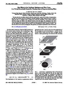
Fig. 1. The PUPs based interpolation scheme proposed by Runions and Samavati [7]. For weight-functions, the method uses a normalized sinc function (A) multiplied by a B-spline basis function (B). Thus, WFs have the form shown in (C). The contour provided in (D) is approximated using the weight-function from panel (C) in (E) and the normalized sinc function in (F).

2.1

Partition of Unity Parametrics

As proposed by Runions and Samavati [7], a Partition of Unity Parametric (PUP) curve Q(u) takes the form: Q(u) =

n X

Ri (u)Ci ,

(1)

i=0

where Ci are control points and each Ri (u) takes the form Wi (u) , Ri (u) = Pn j=0 Wj (u)

(2)

4

CINPACT -splines

where Wi (u) is a Weight-Function (WF) that controls the contribution of Ci to the curve. Dividing by the sum of the WFs normalizes the values of the functions Ri , guaranteeing that they sum to 1. Thus, the Ri are called normalized weight functions. As the Ri provide a partition of unity, the resulting curve must be affine invariant. The final component of the definition of PUPs is the following condition: n X Wj (u) 6= 0 , (3) j=0

which guards against indeterminate forms. To interpolate, for each Pi an interpolation site i is chosen in the parameter domain. Then, Q(i) = Pi is guaranteed through the appropriate choice of Wi . For this purpose, Runions and Samavati [7] proposed the following weight function: Wi (u) = Ii (u)Ai (u),

(4)

where Ii (u) can be any continuous function where Ii (j) = δij , and Ai (u) is a tempering function which must be non-zero at i (i.e. A(i) 6= 0). There are many possible choices for Ii , however they chose Ii (u) =

sin(π(u − i)) , π(u − i)

(5)

the normalized sinc function (Fig. 1 A), which has C ∞ continuity. If this function is supported on the entire domain (i.e. Ai (u) = 1), then the typical artifacts afflicting interpolating curves appear (ringing and overshooting of control points, Fig. 1 F). To temper these effects they used a compactly-supported C k function for Ai (u). When Ii and Ai are multiplied together, the curve is still interpolated, but the support of Ii is smoothly truncated to that of Ai . For Ai (u), they employed uniform B-spline basis functions with variable support (Fig. 1 B). The form of Ii (u)Ai (u) is shown in Fig. 1 C, and a PUPs curve employing this weight-function is shown in Fig. 1 E. The curve produced by the method has a number of properties which are beneficial for geometric modeling: 1. 2. 3. 4. 5.

2.2

affine invariance, resulting from partition of unity normalization, C k smoothness, dependent on the choice of A(u), compact support, dependent on the support of A(u), interpolation, resulting from I(u), and a controllable tradeoff between smoothness and overshooting, by tuning the support of A(u). Zhang and Ma’s method

A class of interpolating curves, related to the preceding PUPs based method, was proposed by Zhang and Ma [10]. Their method employed curves of the form Q(u) =

n X i=0

Ri (u)Ci

(6)

CINPACT -splines

5

with Ri (u) = Ii (u)Ai (u)

(7)

where, again, the normalized sinc function was proposed for Ii (u). In their case, however, the choice of approximating function was 2

Ai (u) = e−α(u−i) .

(8)

It is important to note that in this case normalization by the sum of the weightfunctions does not occur (compare Eqs. 2 and 7), and thus affine invariance is not guaranteed. Nevertheless, for appropriate choices of α, the method produces similar curves to the PUPs based method. When compared to the interpolation scheme proposed by Runions and Samavati, the method proposed by Zhang and Ma has different properties: 1. It offers a tradeoff between approximate affine invariance, and a more focused influence for Ri . Without the normalization step employed above, the Ri ’s do not sum to 1 unless α = 0. At the same time, Zhang and Ma show that the difference from partition of unity is small even when α = 1/3. 2. The curves have C ∞ smoothness. 3. Compact support can only be introduced by forcing Wi (u) = 0 outside of some interval. Thus, it comes at the cost of smoothness. As with affine invariance, the magnitude of the discontinuity introduced by truncating Wi decreases quickly as α is decreased, due to the exponential form of Ri . 4. Interpolation, from the choice of I(u). 5. A controllable tradeoff between smoothness and overshooting, by tuning the coefficient α. Later, Zhang proposed an extension to their method which improved the approximation of partition of unity by introducing an additional term into their basis functions [11]. Aside from this noteworthy difference, the improved method exhibits the same properties as the original method.

3

Weight functions with C ∞ and local support

Examining the interpolation methods described above we notice the following. Runions and Samavati’s method provides unconditional affine invariance, compact support, and C k continuity (for a given finite k). In contrast, Zhang and Ma’s method provides conditional (or approximate) affine invariance, compact support and C ∞ continuity. This raises the following question: can we obtain a method with the positive characteristics of both methods? Specifically, can we support unconditional 1. 2. 3. 4.

affine invariance, C ∞ continuity, compact support, and interpolation,

6

CINPACT -splines

5. while providing a controllable tradeoff between smoothness and overshooting? To answer this question we use the PUPs framework and follow the methodology employed by Runions and Samavati. Namely, given a set of properties we will seek an appropriate weight-function to satisfy these conditions. The construction of PUPs satisfies condition (1). We thus seek an appropriate weight-function with the same form as Equation 4. As in the methods presented in Section 2, we use the normalized sinc function for I(u), which satisfies condition (4). Thus, it remains to choose our A(t) to satisfy constraints (2), (3) and (5).

A

C

k = 0.25 k=1 k=3 k=9 k = 27

B

Fig. 2. The form of bump-functions described in the text, dashed vertical lines indicate the radius of support (i.e. x = ±c). (A) The one sided function from Eq. 9. (B) The two-sided bump function from Eq. 10. (C) A family of bump functions created using Eq. 11 by varying k.

These conditions can be satisfied by identifying an A(t) with C ∞ , and variable compact support. To motivate our choice of weight-function, we first examine the function  f (x) =

1

e− x x > 0 , 0 otherwise

(9)

which is shown in Fig. 2A. This function is zero for negative x-values and smoothly approaches 0 as x → 0+ (i.e. all derivatives approach zero). Thus, the support of this function is smoothly truncated to positive x values. To limit the support of our function to an interval [−c, c], while maintaining C ∞ continuity, we modify the denominator of the exponent to introduce singularities at ±c: ( −1 c2 −x2 x ∈ (−c, c) f (x) = e , (10) 0 otherwise which is shown in Fig. 2B. Now our function f (x) has the desired properties: controllable compact support with C ∞ smoothness.

CINPACT -splines

7

To obtain the A(u) used in our interpolation scheme we modify the above form slightly to obtain: ( −ku2 c2 −u2 u ∈ (−c, c) A(u) = e , (11) 0 otherwise where k is a continuous degree-like shape parameter, which can be used in tandem with the radius of support c to obtain a controllable tradeoff between smoothness and overshooting. The form of A(u) differs from the f (x) in Equation 10, due to the introduction of ku2 into the numerator of the exponential term. This modification gives A(u) a Gaussian-like form (see Fig. 2 C). The resulting interpolation scheme is demonstrated in Figure. 3, where it is used to reproduce cursive handwriting samples of the words July, August and September. CINPACT splines inherit from PUPs the ability to modify the parameters of weight functions on a per-control-point basis (c.f. Fig. 6 in [7]). This permits refined control over the character of the curve without requiring the introduction of additional control points. In Figure 4 this permits the spades symbol (A) 1 to be produced with a small number of control points (B), which account for the sharp protrusions and clefts along contour as well as the differences in the character of the blade and handle. In comparison, using the scheme of Zhang et al. [10], more points are required to approximate the form from (A) with the same fidelity (see C and D).

4

Specifying tangents and higher derivatives of a curve

The ability to specify tangents at control points is important for many CAD applications, such as the design of fonts [4], and illustrations in professional software packages such as Adobe Illustrator. Additionally, curves with tangent control are widely employed in computer animation [6] (e.g. for keyframing). This problem was not addressed by the methods proposed by Runions and Samavati [7] or Zhang and Ma [10], which limits their utility. Here, we address this problem for CINPACT and PUP splines by deriving a method for interpolating tangents and higher order derivatives. We first note that, given the formulation of PUPs in Eq. 4, we can add a sum of weighted vectors to the equation without violating partition of unity (i.e. the resulting curve is still affine invariant). This property is exploited to specify the tangents T0 , T1 , · · · , Tn at the control points of a PUPs curve, yielding the following form n n X X QT (u) = Ri (u)Pi + Ei (u)Vi , (12) i=0

i=0

where Vi are the vectors we add to the curve to meet our tangent constraints and Ei are weight-functions localizing the contribution of these vectors 2 . For 1

2

The spade symbol in Figure 4A was obtained from http://commons.wikimedia. org/wiki/File:French_suits.svg. Note that as Vi are vectors the Ei ’s do not need to sum to 1.

8

CINPACT -splines

Fig. 3. Cursive writing generated using Interpolating CINPACT curves. The curves spell out the words July, September and August. The bump function used in these curves has radius of support c = 10 and shape parameter k = 10.

B

C

D

A

Fig. 4. Comparison of CINPACT curves to those produced using the method of Zhang et al. [10]. A spades symbol (A) is reproduced using a CINPACT curve with 15 points (B) as described in the text, and curves from the method of Zhang et al. with 15 (C) and 24 (D) control points. In (B-D) the top row shows each curve and the bottom row shows the curve overlain on the contour from (A).

CINPACT -splines

9

Fig. 5. The weight-function Ei used to interpolate tangents (blue) and its derivative (red). Dashed lines indicate the support of Ei .

simplicity, let us write QT (u) = Q(u) +

n X

Ei (u)Vi ,

(13)

i=0

where Q(u) is the PUPs curve produced when tangent constraints are ignored. The vector Vi is then chosen so that QT (i)0 = Ti ,

(14)

which implies that Ti = Q0 (i) +

n X

Ei (i)0 Vi .

(15)

i=0

In general, this provides a system of equations that, for appropriate choices of Ei , we can solve for Vi . When a global system of equations must be solved, however, the choice of tangent at a given point may globally contribute to the resulting Vi and thus the form of the curve. We note that by introducing three constraints on the form of Ei we can compute the Vi ’s directly (i.e. without solving a system of equations). Additionally, the direct solution we obtain has the added benefit of localizing the impact of tangent constraints on the form of the curve. These three constraints are: 1. The support of Ei is limited to [i − c, i + c] (similar to the CINPACT basis functions). 2. Interpolating tangents should not interfere with the interpolation of positions: Ei (j) = 0 (j ∈ N). (16) 3. Interpolation of a tangent at one site shouldn’t interfere with interpolation at other sites: Ei (j)0 = δij (j ∈ N). (17)

10

CINPACT -splines

Enforcing these constraints simplifies Equation 15 to Ti = Q0 (i) + Vi .

(18)

Vi = Ti − Q0 (i).

(19)

Thus, our Vi become (Fig. 6 A)

Q(ui)’

A

Vi Ti

B

C

Fig. 6. CINPACT tangent interpolation. (A) The curve Q(u) is shown with desired tangent constraints (orange arrows). The computation of Vi (blue arrow) from Q(ui )0 (green arrow) and the tangent constraint Ti is illustrated. (B) The vectors Vi are multiplied by WFs and added to Q(u) to yield QT (u) (red curve). Blue arrows indicate the sum of weighted vectors at each parameter value. (C) The curve QT (u) smoothly interpolates control points and tangents.

It now remains to find an appropriate choice of Ei , which satisfies our three constraints. This problem is simplified by restricting our search to functions of the following form fi (u)gi (u) Ei (u) = , (20) (fi (u)gi (u))0 (i) where (fi (u)gi (u))0 (i) is the derivative of fi (u)gi (u) evaluated at i. In this case it then suffices to choose fi (u) and gi (u) such that: 1. fi (j)gi (j) = 0 (j ∈ N), 2. (fi (j)gi (j))0 = fi0 (j)gi (j) + fi (j)gi0 (j) = δij (j ∈ N). while maintaining compact support and C ∞ smoothness. We note that these conditions are met by setting fi (u) = Ai (u),

(21)

the bump functions from Equation 11, and: gi (u) = u − i.

(22)

CINPACT -splines

11

To enforce the second condition ( (fi (j)gi (j))0 = δij ), we use a radius of support c ≤ 1 (if c ≥ 1 are desired it suffices to use fi (u) = Ii (u)Ai (u), where Ii (u) is the normalized sinc function centered at i). Thus, our tangent interpolation function is simply Ei (u) =

(u − i)Ai (u) . ((u − i)Ai (u))0 (i)

(23)

Note that if we do not wish to constrain the tangent at Pi , then Vi = 0 and the corresponding term Ei (u)Vi can be omitted. With this weight-function, a CINPACT curve that interpolates the specified positions and tangents can be computed in three steps (Fig. 6): 1. Q(u) is evaluated using Eq. 1 and the interpolating WFs proposed in Section 3. 2. Vi is calculated for each Ti (Eq. 19, Fig. 6 A). 3. The sum of weighted Vi ’s is added to Q(u) (Fig. 6 B) to obtain QT (U ) (Fig. 6 C). ∞ As the WFs used for the control Pn points and the tangents are C with compact support (and by definition j=0 Wj (u) 6= 0), the resulting curve is as well. The basic construction employed to specify the first derivative at i (i.e. the tangent) generalizes to higher order derivatives in a straightforward manner. In particular, to specify Di,n the nth derivative at i we simply set gi (x) = (x − i)n , and Vi,n to (n) Vi,n = Di,n − Qn−1 (i) (24)

where Qn−1 is the curve resulting from the interpolation of the n−1th derivatives (note that Q1 = QT ). This generalized construction is analogous to a Taylor series expansion about the parameter value i, with the impact of the series’ contribution to the curve localized by the support of Ai (x).

A

B

C

Fig. 7. The contour in panel (A) is reproduced using the tangent interpolation scheme (B,C). Tangents are visualized as orange arrows and control points as orange spheres. The resulting curve is shown with (B) and without (C) visualizing tangents.

The method for specifying tangents is demonstrated in Figure 7. In the figure, the contour provided in (A) is reproduced using the control points and tangents shown in (B). Using tangent constraints we are able to approximate the contour using 27 control points (compared to Fig. 1 E where 49 control points were used).

12

CINPACT -splines

In some instances it is cumbersome to specify the tangent at each point (e.g. interactive curve modeling). In such instances, to ease the specification of curves which interpolate a position and tangent, it is useful to generate tangents automatically, from the given set of control points. The Catmull-Rom spline [2], widely employed within computer animation, is a relatively popular method for achieving this goal. These curves are cubic Hermite splines [3, pp. 102–106], where the tangent at each control point Pi is calculated from the neighboring control points Pi+1 − Pi−1 . (25) Ti = 2 In Figure 8 (A), an interpolating CINPACT spline with tangents calculated using Equation 25 is compared to the corresponding Catmull-Rom spline. The curves approximate the contour provided in Figure 7 (A). Note that the CINPACT spline has more evenly distributed curvature, which, in this case, better approximates the original contour (compare panels Figure 8 (B) and (C) with Figure 7 (A)).

A

B

C

Fig. 8. The contour from Figure 7 (A) is reproduced using a Catmull-Rom spline (red contour) and a CINPACT spline (black contour) with the same tangents specified at each control point. In (A) the curves are overlaid and visualized with the control points and tangent vectors. The curves are shown individually in (B) and (C).

5

Approximating curves

Our function A(x) has a plot similar to that of a B-spline basis function. Given this, it makes sense to examine the curves generated by the weight-functions Wi (u) = A(u − i),

(26)

which produces curves that approximate control points. The resulting curves are well-behaved, exhibiting affine invariance, compact support and C ∞ continuity. Furthermore, as shown in Fig. 9 the curves are similar in character to B-splines. Here, however, the parameter k serves as a continuous degree-like parameter. To quantify this statement we have numerically fit W (u) to uniform B-spline basis functions of different orders. Measuring the goodness of fit requires a measure of

CINPACT -splines

13

distance between two functions. To this end we employ the commonly used L2 norm for functions: 1/2 Z ∞ (f (u) − g(u))2 du . (27) d(f, g) = −∞

Using this distance we can estimate the relative error of the fit of the weight function W (u) to the degree d B-spline basis function B d (u) with the following equation d(W, B d ) RelativeError(W, B d ) = , (28) d(0, B d ) where the division by the distance between B d and the constant function 0 normalizes the distance between W and B d . The results of our numerical fitting are reported in Table 1. We observe that by varying k and the support c we can approximate B-spline basis functions of increasing order very well. The particular values of k and c have been determined by numerical optimization, and for B-spline basis functions of degree 2 and higher we obtain small differences between our weight-function and the basis function (less than 0.7% for d > 2). The close correspondence between the forms of CINPACT and B-spline curves is illustrated in Figure 9 for quadratic (A-C) and cubic (D-F) B-spline curves. While the overall approximation is very good, the CINPACT curves, being C ∞ , exhibit less variation (as seen in inset of the bunny tail shown in C). d(W, B d ) k value radius of support c scalar weight Relative error 0.0499 38.94 3.976 0.916264 0.06 0.0122 25.83 3.898 0.761562 0.016 0.0025 17.27 3.684 0.662606 0.0036 0.0021 28.48 5.158 0.599502 0.0032 0.00055 28.00 5.574 0.549665 0.00088 0.0018 23.83 5.560 0.509389 0.0029 0.0033 21.31 5.626 0.476678 0.0056 0.0020 39.84 7.587 0.477571 0.0034 8 0.5683 0.0038 21.05 5.919 0.450372 0.0067 0.00097 33.46 7.365 0.452382 0.0017 9 0.5538 0.0015 31.94 7.579 0.429608 0.0027 Table 1: Parameter values for the best-fit C ∞ weight-functions W for B d , the Bspline basis of degree d. The second column shows the distance between each B d and the constant function 0. The distance between B d and the best-fit W is shown in the third column, with corresponding parameters for W given in the next 3 columns. The final column provides the relative error of the fit (i.e. d(W, B d )/d(B d , 0)). Degree 1 2 3 4 5 6 7

d(B d , 0) 0.8165 0.7416 0.6924 0.6561 0.6276 0.6044 0.5850

These results show that uniform B-spline functions differ only slightly from a C ∞ function with a reasonably simple form. Conversely, this also means that when the parameters k and c are chosen appropriately, the resulting CINPACT curves can be subdivided using B-spline filters with a relatively small error.

14

CINPACT -splines

More broadly, these results show that CINPACT splines, like PUPs, can be used to generate high quality approximating as well as interpolating curves. This can be contrasted against the methods proposed by Zhang and Ma. [10, 11], which only support interpolation.

A

B

C

D

E

F

Fig. 9. A comparison of CINPACT and B-spline curves. (A) A CINPACT curve created from WFs with k = 25.83 and c = 3.898. (B) The curve from (A) is compared to the quadratic B-spline curve generated by the same control points (red curve); the inset is shown in (C). (D) A CINPACT curve created from WFs with k = 17.27 and c = 3.684. (E) The curve from (D) is compared to the cubic B-spline curve generated by the same control points (red curve); the inset is shown in (F).

6

Conclusions

In this paper we have presented CINPACT-splines, which support interpolation and approximation of control points. The resulting curves have a simple, piecewise exponential form. These splines are generated using a class of bumpfunctions as WFs, and guarantee that the resulting curves are C ∞ , with compact support and affine invariance. In this sense, the interpolating CINPACTsplines are an improvement on the previously proposed interpolation methods of Runions and Samavati [7] and Zhang and Ma [10, 11]. Additionally, we provide a method for the interpolation of tangents, a common requirement for the curves used in animation and interactive modeling applications. This, in particular, was not considered in the works of Runions and Samavati [7] and Zhang and Ma [10, 11].

CINPACT -splines

15

The approximating CINPACT-splines behave similarly to B-splines, but do not sacrifice continuity in order to achieve compact support. Additionally, the shape parameter k provides a continuous degree like parameter. Consequently, unlike B-splines, the weight-functions are not defined by a recursive relation, but have a simple closed form. Furthermore, when curve fitting is performed the parameter k and radius of support c can be independently optimized as continuous parameters. In contrast, for B-spline curves the degree determines the support, and when optimized during curve fitting introduces a discrete parameter. These advantages highlight the potential of CINPACT-splines as an alternative to Bspline curves. As the curves considered by Runions and Samavti [7] employed b-spline basis functions CINPACT-splines likewise offer a number of advantages over the curves considered in [7]. By employing closed form exponentials (bumpfunctions) in place of b-spline basis functions our curves have a relatively simple implementation, but can still provide the basis for a comprehensive curve modeling package. A key goal of future work on CINPACT-splines will be to further examine their relation to B-splines. In this paper we considered the fitting of CINPACT weight-functions to uniform B-spline basis functions, which assume a uniform spacing of knot values. It is an open question, however, what class of bumpfunction is required to reproduce arbitrary B-spline basis functions (i.e. those generated by non-uniform knot values). A related problem is the local refinement of weight-functions, which for B-splines is accomplished through knot insertion [1]. Pursuing these two directions should allow CINPACT and B-splines to be used interchangeably, opening the door to their widespread use in CAD applications.

References 1. Bartels, R., Beatty J. and Barsky B. (1987) An Introduction to Splines for Use in Computer Graphics and Geometric Modeling. Morgan Kaufmann, Los Altos, California. 2. Catmull E. and Rom R. (1974), “A class of local interpolating splines.,” In: Computer Aided Geometric Design, pp. 317-326. 3. Farin G. (2002), Curves and Surfaces for CAGD. Morgan Kauffmann, San Francisco, CA. 4. Knuth D. (1995), The METAFONT Book. Addison-Wesley, Boston, MA. 5. Lee J. (2000), Introduction to Smooth Manifolds. Springer, New York. 6. Parent R. (2012), Computer Animation. Morgan Kauffmann, San Francisco, CA. 7. Runions A. and Samavati F. (2011), “Partition of Unity parametrics: A framework for meta-modeling,” The Visual Computer, 27:495–505. 8. Sederberg T., Zheng J., Bakenov A., Nasri A.(2003), “T-splines and T-NURCCs,” ACM Trans. Graph., 22:477–484. 9. Wang Q., Hua W., Guiqing L., Bao H. (2004), “Generalized NURBS curves and surfaces,” In: Geometric Modeling and Processing, pp. 365-368. 10. Zhang R.-J. and Ma W. (2011), “An Efficient Scheme for Curve and Surface Construction Based on a Set of Interpolatory Basis Functions,” ACM Trans. Graph., 30: 10:1–10:11.

16

CINPACT -splines

11. Zhang R.-J. (2012), “Curve and surface reconstruction based on a set of improved interpolatory basis functions,” Computer-Aided Design, 44: 749-756.