Sung-Soo Kim and Chong-Min Kyung, Member, IEEE. Abstract-In this paper, we present an algorithm, called self- organization assisted placement (SOAP), ...
844
IEEE TRANSACTIONS ON COMPUTER-AIDED DESIGN, VOL. 11, NO. I, JULY 1992
Circuit Placement on Arbitrarily Shaped Regions Using the Self-Organization Principle Sung-Soo Kim and Chong-Min Kyung, Member, IEEE
Abstract-In this paper, we present an algorithm, called selforganization assisted placement (SOAP),for circuit placement in arbitrarily shaped regions, including two-dimensional rectilinear regions, nonplanar surfaces of three-dimensional objects, and three-dimensional volumes. SOAP is based on a learning algorithm for neural networks proposed by Kohonen [l], called self-organization, which adjusts the weight of synapses connected to neurons such that topologically close neurons become sensitive to inputs that are physically similar. In contrast to earlier methods on circuit placement in rectilinear region, where the final placement heavily depends on an arbitrary partition of the entire region into a number of rectangular subregions, thus leading to suboptimal results, SOAP is a general algorithm for circuit placement in arbitrarily shaped regions without these drawbacks. A standard cell placement method and a global placement method of macro cells using SOAP algorithm are also described. Several examples showing the circuit placement on rectilinear regions, nonplanar surfaces, and 3-D volumes are shown. Experimental results on benchmark circuits show that the SOAP algorithm is competitive with the state-of-the-art algorithms even for the case of placement in a rectangular region, which is a special case of a 2-D rectilinear region.
I. INTRODUCTION LSI technology has matured to the extent where hundreds of thousands or even millions of transistors can be integrated on a single chip, forming the key to the design of efficient electronic systems. As IC chips become more complex, more efficient layout tools are necessary to obtain good layout and reduce the turnaround time. VLSI layout refers to the transformation of the functional and logic specifications of a desired chip to a physical realization of transistors, cells, and macros together with their interconnection pattern. A general overview of circuit layout is given in [2]. Because of the inherent computational complexity of the layout problem, the overall layout problem is divided into subproblems : partitioning, floor planning, placement, global routing, detailed routing. The placement problem involves placing circuit modules on a chip in a nonoverlapping manner in such a way as to maximally preserve the intermodulate connectivity, thereby maximizing the routability of the chip and mini-
V
Manuscript received January 8, 1990; revised October 15, 1990. This paper was recommended by Associate Editor R. H. J. M.Otten. The authors are with the Department of Electrical Engineering, Korea Advanced Institute of Science and Technology, 373-1 Kusong-Dong, Yusung-Gu, Taejon, Korea. IEEE Log Number 9105855.
mizing the area required. It has been shown that the placement problem is NP-hard [3]. The computation time required to obtain the optimum solution increases exponentially as the number of modules increased [4]. Many algorithms based on heuristic rationales have been developed to obtain a nearly optimum solution in a reasonable time [5]-[8]. Placement methods fall into two classes: constructive and iterative. Constructive methods include cluster growth [9]-[ 113, partitioning-based placement [ 121-[16], and the analytical method [17]-[22]. The cluster growth algorithm selects an unplaced module based on an evaluation function which measures signal net connectivity to modules already or not yet placed, and then decides the best position for it relative to the modules already placed. This process is repeated until all modules are placed. The top-down partitioning algorithm divides the global modules into subsets such that the number of weighted connections among the subsets is minimized and the area of the modules in each subset is more or less uniform. The analytical method models the placement problem as a linear or nonlinear optimization problem where all modules are moved simultaneously along an ndimensional gradient in the placement state space. Iterative methods include pairwise interchange [5], force-directed interchange and force-directed relaxation [5], simulated annealing [23]-[25], evolution [26], and the genetic method [27]. In the pairwise interchange method, two modules in a layout are interchanged and the cost function of the new layout is computed. If there is an improvement, the new layout replaces the old one; otherwise it does not. Force-directed interchange and force-directed relaxation methods use force to determine the position to which the selected modules should be moved. These iteration methods accept the ‘next configuration only if the objective function does not increase. This property may cause the results to fall into a local minimum. Simulated annealing (SA) uses a probabilistic hill-climbing method to avoid local minima. In the SA, one cell is moved or two cells are exchanged in one iteration. If the movement reduces the objective function, the movement is accepted. If the movement increases the objective function, the movement is accepted or rejected based on the Boltzmann distribution function. ESP [26] and the genetic method [27] are similar to SA. The basic idea of ESP is to keep the cells which are already well placed in their present locations and to improve the positions of the badly placed cells. The goodness of the placement of a cell is deter-
0278-0070/92$03.00 0 1992 IEEE
845
KIM AND KYUNG: CIRCUIT PLACEMENT ON AN ARBITRARILY SHAPED REGION
mined with the degree of clustering of its neighboring cells. The genetic method maintains a large population of configurations during the iteration and each new configuration for the next generation is constructed from the two previous configurations. Most of the above algorithms are targeted to circuit placement in a rectangular region. In practical layout problems on a PCB (printed circuit board) or in VLSI, the shapes of the layout regions are not necessarily confined to rectangular ones. For example, PCB’s are often defined to be nonrectangular by the constraints arising from the moving or nonmoving mechanical parts nearby. In VLSI layout, the available layout regions become rectilinear because of the preplacement of certain large macro cells, such as ALU, PLA, and ROM, on the original rectangular chip surface. Previous work [28], [29] on the placement of circuit modules in a rectilinear region has simply used the conventional rectangular region placement algorithm after the entire rectilinear region has been divided into a number of rectangular subregions. Such region-partition-based methods could lead to poor results since the final placement depends heavily on the region partitioning, for which no clear criteria exist. ACG [lo] is an algorithm that places circuit modules in a rectilinear region without region partitioning, but it requires, as its input, the result of a global placement which can be done by using such techniques as FDR [ 171 and FOCUP [53]. Recent advances in artificial neural network research provide new techniques for pattern recognition, optimization problems, and other applications [30]-[35]. The computational power of artificial neural networks comes from the massively parallel operation of a large number of simple processing elements (neurons) with a large number of interconnections (synapses) between neurons. Recently, impressive results were obtained by applying neural network models to various optimization problems in VLSI design [36]-[48]. Algorithms have been developed for circuit placement based on the Hopfield model and Kohonen’s algorithm [37]-[48]. The Hopfield model [31] is a neural network which has a symmetrical interconnection matrix and a sigmoid gain function. When the gain function approaches the step function, the Hopfield network converges to a local minimum of an energy function. Naft [39] adapted the Hopfield neural network model for the traveling salesman problem (TSP) to multiobjective component placement based on wire length criteria and thermal reliability. Caviglia et al. [41] proposed a modified Hopfield network for block placement with the objective function of bounding box minimization, connection length minimization, and overlap removal. Yu [44] tried to obtain a placement result using the Hopfield model, but not with great success. Sriram and Kang [48] introduced a modified Hopfield network for a two-dimensional module placement problem. They adopted a hierarchical placement approach by applying the technique of min-cut quadrisection [16] at each stage. Kohonen’s selforganizing principle [l] is an unsup&ised learning al-
....
gorithm for neural networks. The algorithm produces what he calls self-organizing feature maps, in which the weight vectors between input nodes and output nodes tend to approximate the distribution of input vectors in an orderly fashion. Circuit placement using Kohonen’s algorithm has already been described by the authors [37]. Caviglia et al. [46] used Kohonen maps for preplacement by recursive bipartitioning of the circuit. Zhang and Mlynski [47] proposed a placement algorithm using a topology mapping property of a neural model suggested by Kohonen and Ritter. In their algorithm, the movable modules are mapped into the predefined slots on a chip. In this paper, we describe an algorithm, called self-organization assisted placement (SOAP), for circuit placement in arbitrarily shaped regions, including nonrectangular planar or nonplanar layout surfaces, and even for three-dimensional placement. A standard cell placement method and a new global placement method for macro cells using the SOAP algorithm are also described. For the macro cell placement, a modified SOAP algorithm is introduced where the sizes of modules are considered during the self-organization process to reduce the overlaps among modules. The orientations and rotations of modules are also considered in the macro cell placement. The organization of this paper is as follows. The basic SOAP algorithm is described in Section 11. Standard cell placement on arbitrarily shaped planar surfaces using the SOAP algorithm is described in Section 111. In Section IV, we describe the global placement of macro cells with a modified SOAP algorithm. In Section V, circuit placement on nonplanar surfaces and in 3-D volumes using the SOAP algorithm is described. Experimental results are discussed in Section VI. 11. SELF-ORGANIZATION ASSISTEDPLACEMENT Circuit placement on arbitrarily shaped planar surfaces using SOAP consists in finding the positions of circuit modules within the specified region such that the closely related modules are placed near one another, or, loosely speaking, the whole interconnection length is minimized. The relationship between Kohonen’s model and the proposed placement model is described in Fig. 1, where output nodes correspond to circuit modules. Connections between output nodes in the neural network correspond to signal nets connected to the corresponding modules in VLSI circuits. The number of input nodes corresponds to the dimensionality of the circuit placement region. Variable connection weight from input node sito output node rj, denoted by wij, corresponds to the ith coordinate value of the position of module mj.(The first and the second coordinates two-dimensional in the space are the x and the y axes, respectively.) Training input vectors in the neural network correspond to randomly selected points in the legal placement region. In this algorithm, circuit modules are numbered from 1 to N and the position of each module i is denoted by a vector:
K
=
{wli, W Z } -
IEEE TRANSACTIONS ON COMPUTER-AIDED DESIGN, VOL. 11, NO. I, JULY 1992
a46 Y '
signalnet
Step 1. Initialization : r SO.
Cells are clustered around the center of region. Step 2. Present a new input
. ........
Wi
X(1) = {X,(~)&(OI
Step 3. Select the cell j which is newest hum the input, X(rJ, i.e., select j' such that
i
inmtnode
(k1-w,,)'+ c%-w2JZl is minimal when i =j'.
Step 4. Update the position of cell j' and its neighbors within the distance of
Fig. 1. The correspondence of items between (a) Kohonen's model and (b) the placement algorithm. Output nodes (r,'s) in Kohonen's model correspond to circuit modules (m,'s) in the placement algorithm. The variable connection weight from input node s, to output node r,, denoted by w,,, corresponds to the ith coordinate value of the position of module m,. (The first and the second coordinates in the two-dimensional space are the x and they axes, respectively.) Connections between output nodes correspond to intermodule connections.
wli
= w,, +
w,
=
W~
N r A .k , W - w , J
+ q(r.I).(&(r)-wd
where a@). q(rj) (0 e q(rj) e 1) are neighborhood function and gain function, respectively,and r is the distance of cell i from cell
,'.
Step 5. Increment 1. Step6.
In the case of placement on a planar surface, the number of components of vector W i(for all i) is 2, where wli and w2idenote the x and y coordinate positions of the ith module, respectively. (We need wli additionally for the placement on nonplanar surfaces to represent the z coordinate value.) The proposed circuit placement algorithm, SOAP, is described in Fig. 2. Initially, all the circuit modules are clustered around the center of the region by setting the position vector of all modules to small random values around 0. (The center location is represented as (0, O).) These position vectors are then trained (modified) during the self-organization process by the input vectors, which are uniformly distributed over the whole allowed placement region. Input vectors are presented one by one. Whenever an input vector is presented, Euclidean distances from the input vector to all the position vectors are calculated and we find the module, j * , for which the Euclidean distance is the smallest. The positions of the modulej* and other modules in its neighborhood are modified to make these modules more responsive (closer) to the current input. Fig. 3 shows this process. Fig. 3(a) shows an input point and Euclidean distances from the input to all the modules. Here, the selected module, i.e., module 2, which has the smallest distance, is shown as a shaded circle. In Fig. 3(b), the movement vector is represented by arrows showing the direction and the magnitude of the movement of the selected module and its neighboring modules to be moved together. Neighborhood NEj ( t ) of a module j at time t is a set of modules lying within the distance a(t) from the modulej, where o(t) is a time-decreasing function which determines the size of the neighborhood. Fig. 4 shows the topological neighborhood of a circuit at different time instances. If a module, i, lies within the neighborhood of the modulej", the position of module i is updated using the following rule (Step 4 in Fig. 2):
U(I)
h m the cell j'. Le., for all such cells, i, p e r f o r m
IfO(i)=O.O
Stop.
ElSe
Go to Step 2.
&
Fig. 2. SOAP (self-organization assisted placement) algorithm.
t
input point
* a ..
4
I (a)
(b)
Fig. 3. Position update process. (a) Distances from the input point to all cells are calculated and the nearest cell is selected. (Cell 2 is selected, since r 2 < rl < r4 < r3.) (b) Nearest cell (2) and its neighbor cells (1, 3 , 4) are moved toward the input vector position with the magnitude indicated by the length of the arrows.
NE Itl')
--
'..........\......\ .''.q
Fig. 4 . Topological neighborhood at different time instances. The size of the neighborhood is initially large and slowly decreases over time. For ) 1, and 4 3 ) = 0 for r l < r2 < r3, respecexample, o(t1) = 2, ~ ( r 2 = tively, in this figure.
KIM AND KYUNG: CIRCUIT PLACEMENT ON AN ARBITRARILY SHAPED REGION
i
847
0.4
OiE 0.25 0.2 0.1 5 0.1
0.05 n "
-5 -3
-1
1
3
-'r
5
Fig. 5 . Gain term, ~ ( rr),, versus r with different values of
U.
where the gain term, q(r, t ) , is a slowly decreasing function of time ( r being the topological distance between module i and module j * , e.g., r = 1 for the modules directly connected to module j*,etc.) and is defined as follows:
where N is the size of the initial neighborhood. The shape of the gain term, q(r, r), in (2) versus r is shown in Fig. 5 with different values of 0. Fig. 5 shows that the distances of the movement of cells decrease as time increases (since a(t) is a time-decreasing function); that is, the topological distance to the selected module, r, increases. Therefore, the positions of modules eventually converge and are fixed after the gain term is reduced to 0. In the case of circuit placement with input/output (I/O) constraints, the I/O ports are regarded as fixed modules located at a specified position on the boundary of the region. These 110 modules are not moved during the process of the SOAP algorithm but can be selected as the nearest module from a given input vector as inner modules. Especially in the early stage of the process, I/O modules affect the distribution of the internal modules by giving a direction of the movement of modules having connections with them. 111. STANDARD CELLPLACEMENT USINGTHE SOAP ALGORITHM In the standard cell methodology for IC layout, predefined cells in the library are used in common for various chip designs. Cells in the library have standardized physical patterns, such as cell height, terminal direction and location, and power line location, and are usually arranged in horizontal rows during the layout. Fig. 6 shows a rectilinear standard cell layout region obtained by the preplacement of macro blocks with I/O pads placed around the periphery of the chip. Standard cell placement using the SOAP algorithm comprises three steps: 1) initial placement using basic SOAP algorithm; 2) row assignment of cells; 3) arrangement of cells in each row.
Fig. 6. A rectilinear standard cell layout negion obtained by the preplacement of macro blocks with 1/0pads placed around the periphery of the chip.
In step 1, the basic SOAP algorithm mentioned in Section I1 is used to obtain the initial placement of the inner cells in the rectilinear region with the I/O cells fixed along the periphery. During the initial placement, random inputs uniformly distributed over the entire rectilinear region are generated to obtain the dot patterns uniformly distributed over the entire placement region. In step 2, row assignment of cells is performed. Cells are first sorted according to their y-coordinate values. We then move down a horizontal sweep line from the top of the placement region until the sum of widths of the cells swept is equal to the available row width in the current row. (In a rectilinear region, the row width is a function of the vertical position of the row.) The cells swept by this horizontal sweep line are assigned to the current row while maintaining their relative column positions (x coordinates). After the row assignment of all cells, feedthrough cells are inserted to complete the connections of all the signal nets. After feedthrough cell insertion, the width of each row is calculated including the feedthrough cells. If the deviation of the row width from the available row width in any row is larger than a specified value, line sweeping is performed again, taking into account the number of feedthrough cells in each row. If the deviations of all rows are smaller than the specified value, the x coordinates of feedthrough cells are determined. The x coordinate of a feedthrough cell is determined with the x coordinates of cells connected to the net which runs through this feedthrough cell. Fig. 7 shows a method for determining the x coordinates of the feedthrough cells for various cases. Step 3 involves the arrangement of all the cells in each row without overlaps among cells. This step is performed according to the intrarow cell placement algorithm [ S I . During the process, cells are divided into three groups, i.e., placed cell group, active cell group, and unplaced cell group (see Fig. 8). The placed cell group contains
IEEE TRANSACTIONS ON COMPUTER-AIDED DESIGN, VOL. 11, NO. 7, JULY 1992
848
\
of the left boundary of row i for all i . We then select the row that has the smallest pi. (When a tie occurs, select arbitrarily.) In the selected row, select a cell among the active cells according to the selection rule and move this selected cell to the placed cell group and update piby the amount of the width of this selected cell. Move the front unplaced cell to the active cell group in the selected row. This process is repeated until all the cells are moved into the placed cell group.
/
I””’-’(’” 4
INTl
of feed-through cells
I II
1’1
‘-
\ /
INT2
(C) Fig. 7. Positioning the feedthrough cells in the case of (a) one interval including the other interval, (b) two intervals not overlapped, and (c) two intervals partially overlapped. Shaded boxes represent the cells connected to a net.
row1
row2
row3
Fig. 8. Arrangement of cells in each row. One cell in the active row2 is selected (sincep2 < pl < p 3 ) . The selected cell is represented as a black square. In this case, the number of active cells is limited to 3 (K = 3).
cells already placed. The active cell group contains cells to be placed next. The rest belong to the unplaced cell group. To select a cell in the active cell group, we use a selection rule. New net, terminating net, and continuing net are defined to be used in the selection rule. New net is a connection between an active cell and an unplaced cell. A terminating net is connected to an active cell and placed cells. Continuing net is connected to placed cells and at least two cells among active cells and unplaced cells (see Fig. 8). According to the selection rule [ S I , the cell that maximizes the difference between the number of terminating nets and the number of new nets is selected, with certain tie-breaking rules. First, cells in each row are sorted according to their xcoordinate values and inserted into unplaced cell group. In each row, K cells (Kdenoting the maximum number of cells in the active cell group) from the unplaced cell group are moved into the active cell group. We define pi as the x coordinate of the boundary position between placed cell and unplaced cell in row i . Initially, pi is the x coordinate
IV. GLOBALPLACEMENT OF MACROCELLSUSING SOAP ALGORITHM In the basic SOAP algorithm, each circuit module is considered as a point. As a result, there will be some overlaps among modules in the placement result. This has not been too serious a problem for the placement of standard cells whose size is relatively small and more or less uniform. On the other hand, macro cells have a very large fluctuation of module sizes, and the module size itself is usually not ignorable, as in the case of gate arrays or standard cells. In this section, we describe a modified SOAP algorithm for the global placement of macro cells which considers the size and shape of modules and reduces the overlaps among macro cells. The overall procedure of the global placement algorithm for macro cells using the modified SOAP algorithm comprises five steps: 1) initial placement using the basic SOAP algorithm (where module size is assumed to be zero); 2) gradual expansion of module sizes; 3) rotation and orientation of modules for minimal pinto-pin wiring length; 4) reduction of intermodule overlaps using the modified SOAP algorithm; 5 ) if (current module size is equal to the actual module size) Stop. else Go to step 2.
The basic SOAP algorithm is used to obtain the initial placement. For the initial placement, all modules are considered as points, and the random input vector is generated within the initial placement region, which is about 25% of the entire region,”ak shown in Fig. 9. This strategy has been shown to be superior to the case of spreading the initial placement over the whole region. The initial placement procedure is stopped when modules are sufficiently uniformly distributed in the initial placement region. In step 2, the sizes of modules are increased gradually to preserve the current placement configuration and to reduce the overlaps in the following steps. An abrupt change of module sizes will result in a significant distortion of the current placement, which is generally not desirable. In step 3, reorientations of all modules are performed to minimize the sum of the half-perimeter cost of the minimum bounding box (MBB) of the corresponding nets. Rotation is allowed only in 90” steps. The half-perimeter of nets connected to a cell is calculated as the summation of the Manhattan distances between the pin
849
KIM AND KYUNG: CIRCUIT PLACEMENT ON AN ARBITRARILY SHAPED REGION
n
Original placement region
1 Initial placement region
selected position with minimum overlap m a
I.
I Fig. 9. Original placement region and initial placement region.
dli
Fig. 10. Modified position update method. Module i is moved along the moving direction. The overlap area along the moving direction is checked for some finite increment of A and the position which has minimum overlap area is selected. Y
position and the corresponding net position. The net position is assumed to be at the mass center of the coordinates of pins which belong to the net. Owing to the operation of module expansion and rotation in steps 2 and 3, overlaps among modules usually become larger. To reduce these overlaps, we suggest a modified SOAP algorithm. The modified SOAP algorithm is different from the basic SOAP algorithm in the position update step (step 4 in Fig. 2). In the basic SOAP algorithm, the position of modules is directly updated by the target position calculated with the position update rule. In the modified SOAP algorithm, only the direction of the movement of modules is given by the basic SOAP algorithm. The actual movement is determined such that the amount of overlap with the other modules is minimal. In Fig. 10, the target position of module i as calculated by the basic SOAP algorithm is shown. In the modified SOAP algorithm, the movement vector ( d l l ,&) is reduced by a factor of a,(0 < a, < 1, for all i); i.e., the new movement vector is given by ( d i , , d i l ) = (CY, * d l l ,a, * &), as denoted by the shaded box. The modified update step 4 is as follows:
4) Update the position of cell j * and its neighbors within the distance o(t) from j*.That is, for all such cells, i, perform the following operations: Wlr
= Wlr
+ a, -
v(r,
0
*
(XdQ
- w,,)
+ a, v e ? t ) - (x2(Q - w2r) where a,(0 < a, < 1, for all i) is determined such W2r
= W2r
that the amount of overlap of module i with other modules is minimal. ON NONPLANAR SURFACE AND V. CIRCUITPLACEMENT THREE-DIMENSIONAL VOLUME Many studies on three-dimensional IC [49]-[513 show that three-dimensional implementation of circuits provides such advantages as high packing density, high speed, and parallel operation. The three-dimensional packaging problem was treated in [52]. Recent studies on multilayer, multichip modules [56], multilayer PCB's, three-dimensional packaging [57],etc., clearly show that
wli
X
(a) (b) (C) Fig. 1 1 . Three-dimensional placement (a) on the surfaces and (b) on multiple layers. (c) Position vector of module i in three-dimensional placement.
three-dimensional placement [5 13 will become an extremely serious issue in electronic system packaging in the near future. In this section, a circuit placement on nonplanar, i.e., three-dimensional, surfaces and on multiple layers using the SOAP algorithm will be described. This placement problem on three-dimensional surfaces (see Fig. ll(a)) can occur when the electronic circuitry for the control of certain mechanical objects is to be placed on the interior or exterior surface of the object or when it is necessary to place the circuit modules on the surface of three-dimensional objects to minimize the occupied volume or total wiring distances. The placement problem on multiple layers (see Fig. ll(b)) can occur when various devices or circuit functions, such as photosensors, logic circuits, memories, and CPU's, are arranged in each active layer to achieve high packing density and high functional performance [ 5 8 ] . In the three-dimensional circuit placement, the position of each module i is denoted by a vector W, = {wli, w ~ i , w g i } ,where w l i , wZi,and wli denote the x , y, and z coordinate positions of the ith module, respectively (see Fig. 11(c)). The algorithm for circuit placement on multiple layers follows: Initial placement using the basic SOAP algorithm. Calculate available area of each layer. Current layer = top layer. Sort cells with their y-coordinate values. Move down sweep plane until the area requirement of the current layer is satisfied. Assign cells swept by sweep plane to the current layer.
IEEE TRANSACTIONS ON COMPUTER-AIDED DESIGN, VOL. 11, NO. 7, JULY 1992
850
5 ) If all the cells have been projected, then Stop. else Current layer = next layer. Go to Step 3. In the first step, cells are distributed uniformly over the entire three-dimensional space using the basic SOAP algorithm. In this step, input vectors are generated randomly in the minimum bounding volume that includes all the layers on which cells are placed. These input vectors are used to update the positions of cells in the SOAP algorithm. After initial placement, layer assignment of cells is performed. The layer assignment of cells in the placement on multiple layers is similar to the row assignment of cells in the standard cell placement. First, the available area of each layer is calculated and cells are sorted according to their y-coordinate values. We then move down an n-z sweep plane from top to bottom of the placement space until the sum of areas of cells swept is equal to the available area of the current layer. The cells swept by this x-z sweep plane are assigned to the same layer while maintaining their x and z coordinate values. This process is repeated for the next layer until all the cells are proj ected. The algorithm for circuit placement on nonplanar suris as follows: Initial placement using basic SOAP algorithm. Make sorted cell list for each surface. Select a cell which has the minimum distance among the sorted cell lists. Project the selected cell to the corresponding surface and delete this cell. If the area requirement of this surface is satisfied, then delete all the cells in the corresponding sorted cell list. If all the cells have been projected, then Stop. else Go to Step 3. Initial placement on nonplanar surfaces is equal to the initial placement on multiple layers. In the placement on three-dimensional surfaces, a sorted cell list at each surface is required for the projection of cells on the surfaces. In the sorted cell list of a surface, cells are ordered with the distances from their positions to the position of the corresponding surface. Among the sorted cell lists, the cell which has minimum distance is selected and projected to the corresponding surface. The projected cell is removed from all the sorted cell lists. If the area requirement of this surface is satisfied, all the cells in the sorted cell list of this surface are deleted. This process is repeated until all the cells are projected. Simple experimental results on three-dimensional placement are given in Section VI.
RESULTSAND DISCUSSION VI. EXPERIMENTAL In this section, we describe experimental results of the placement of example circuits. The SOAP algorithm was implemented in C on SUN4. Table I shows the characteristics of the example circuits. Primaryl, Primary2,
TABLE I NUMBERS OF MODULES, NETS,AND I/O PADSFOR TESTCIRCUITS Circuit
Modules
Nets
Pads
ALU ami33 [54] DECIN [54] REGFILE [54] Primaryl [54] Primary2 [54]
61 33 138 160 752 2901
81 123 150 196 904 3029
22 42 48 196 81 107
DECIN, and REGLE are taken from the benchmark data [54]. Fig. 12 shows the placement result of an example circuit called ALU in a rectangular region. Fig. 12(a) shows the time behavior during the SOAP process. The initial positions are clustered at the center, as shown in l ) , and finally spread out over the whole region, as shown in 6). Fig. 12(b) shows the change of half-perimeter routing length versus iteration number during the placement of ALU where the cost is obtained by converting the dot distribution into the module placement using the FOCUP algorithm [53]. In Fig. 12(b), we can see that the cost variation at the early stage is high and is gradually degraded as the process continues. It is seen that the cost eventually converges, more or less, to some constant value. The large variation of cost at the early stage is due to two factors. First, a relatively large number of modules are moved around an input vector since the size of the neighborhood is larger at the beginning than at the end. Second, the moving distance of the module is large in the beginning since the gain term, q , is also large. As the process goes on, however, these effects are reduced because the size of the neighborhood and the magnitude of the gain function are decreased. Fig. 13 shows the time behavior of block placement in an arbitrary rectilinear region for an example circuit called ALU using the SOAP process. It is shown that the modules gradually occupy the available placement region maintaining a more or less uniform population density and keeping the strongly connected modules near one another. Fig. 14 shows the placement result of a benchmark circuit called Primaryl [54] in a rectilinear region. In this case, modules were placed in 20 rows with a channel height of 220 pm. Fig. 14(a) shows the dot pattern of Primaryl obtained by the SOAP algorithm. Fig. 14(b) shows the final result obtained after row assignment and determination of positions of cells in each row using the standard cell placement algorithm explained in Section 111. Next, we show the result of running the modified SOAP algorithm on certain macro cell circuits, which was explained in Section IV. Fig. 15 shows the time behavior of module placement for an example circuit having 4 x 4 mesh connected modules. For each increment of time, it is shown that the sizes of modules are gradually increased until they reach their final sizes at t = t6, and the placement configuration is gradually converging to the optimal one. Fig. 16 shows the result of running the modified
85 1
KIM AND KYUNG: CIRCUIT PLACEMENT ON AN ARBITRARILY SHAPED REGION
3.8 3.7 3.6
3.5 3.4 3.3 3.2 3.1
I
0
I
2
I
I
I
4
1
1
I
6
8
I
I 10
Iteration Number ( x 1000 ) (b) Fig. 12. Circuit placement result of ALU having 67 modules in a rectangular region. (a) Time behavior showing self-organization. (b) Change of half-perimeter routing length versus iteration number during the placement of ALU.
.......
.
o
0
-
m m
(a) Fig. 13. Intermediate phases of block placement in rectilinear region for ALU .
0
.
m . .
(b)
Fig. 14. Block placement result in rectilinear region for Primaryl: (a) msult of SOAP algorithm: (b) detailed circuit placement result of (a).
852
IEEE TRANSACTIONS ON COMPUTER-AIDED DESIGN, VOL. 11, NO. 1, JULY 1992
'2
5
'4 Fig. 15. Time behavior of module placement for an example circuit having 4 X 4 mesh connected modules. For each increment of time, it is shown that the sizes of the modules are gradually increased until they reach their final size at t = t6, and the placement configuration gradually converges to the optimal one.
~
Fig. 16. Placement result of benchmark circuit called ami33.
SOAP algorithm on a more complex benchmark, called ami33. In the initial stage of the modified SOAP algorithm, module orientation is first performed, as mentioned in Section IV, such that the half-perimeter cost of the minimum bounding box of all the nets connected to the current module is minimal. Finally, we have some experimental results on circuit placement on nonplanar surfaces and three-dimensional circuit placement. Fig. 17 shows an example of module placement for an artificial circuit where the modules are connected in three-dimensional fashion as shown in Fig. 17(a) on multiple layers. After running the SOAP algorithm on multiple layers, which was explained in Section V, the optimal solution is obtained. An example of applying the SOAP procedure to the circuit placement in nonplanar surface is given next. An exploded view of the block placement results on the six surfaces of a cube for the circuit ALU is shown in Fig. 18 in order to demonstrate the capability of the SOAP algorithm for placing circuit modules in three-dimensional space. Fig. 18(a) shows the overall module distribution and the net connec-
(a) (b) Fig. 17. An example of three-dimensional circuit placement on multiple layers: (a) example circuit; (b) optimal result.
tion pattern drawn as spanning trees. Fig. 18(b) shows the nets which connect only the modules on the same face. Parts (c) and (d) of Fig. 18 show the nets which connect the modules only on the neighboring faces and only on opposite faces, respectively. In Fig. 18, we can see that modules are, more or less, uniformly distributed over all surfaces and that modules to be connected are close to one another. Only one out of 81 nets was placed such that the modules belonging to this net were placed on opposite faces, as shown in Fig. 18(d). SOAP is a very general algorithm applicable to widely varying types of placement regions, and it cannot be directly compared with other placement algorithm applicable only to very limited types of placement regions, typically 2-D, rectangular region. However, for purposes of comparison, two benchmark circuits, Primary 1 and Primary2, were run on a rectangular region with consideration of I/O pads. The modules were placed in 17 and 26 rows, respectively, with estimated channel height of 220 pm and 270 pm. For the placement of Primary1 and Primary2, 10 000 and 5 were used as the number of total input vectors and the size of initial neighborhood in the SOAP algorithm, respectively. The elapsed CPU times were 300 and 800 s, respectively, on SUN4 (10 MIPS machine). In Table 11, the half-perimeter routing lengths of min-cut, RT, Gordian, and SOAP algorithms are compared using the same benchmark circuits. Data from the first three methods in Table 11, i.e., min-cut with terminal propagation [ 141, RT: the relative placement/transportation [21], and Gordian [22], were obtained from [22]. It is seen that the performance results of the SOAP algorithm are quite comparable to those of other heuristic algorithms which are applicable only to rectangular planar regions, for the case of placement in a rectangular chip region. The placement results of DECIN and REGFILE using the SOAP algorithm without consideration of U 0 pads are also shown in Table 11. The modules in DECIN
853
KIM A N D KYUNG: CIRCUIT PLACEMENT ON AN ARBITRARILY SHAPED REGION
0
0
O
0 Q
0 )
20 (a)
(b)
(C)
A
(d)
Fig 18 Exploded vlew of block placement and the connectlon pattem on the surface of a cube using self-organization (a) Total wires Wires (b) within a face, (c) in neighbonng faces, and (d) In opposite faces
TABLE I1 EXPERIMENTAL RESULTS FOR PRIMARY 1, PRIMARY2. DECIN, A N D REGFILE Circuit
min-cut
RT
GORDIAN
SOAP
Primary 1 Primary2 DECIN REGFILE
1739 9823 -
2177 8685 -
-
-
1503 8142 -
1564 8465 103.73 66.65
were placed in six rows with expected channel height of 150 pm, and the modules in REGFILE were placed in eight rows with expected channel height of 20 pm. For the placement of DECIN and REGFILE, 4 and 2 were used as the size of the initial neighborhood, respectively, with the total number of input vectors being 4000. The elapsed CPU times were 39 and 24 s, respectively. The optimum placement configuration of the REGFILE is that all the cells connected to each net are arranged in a row or a column with a half-perimeter routing length of 43.96 mm. REGFILE is very regular (register file) and is unlikely to be laid out using autoplacement tools. Because the proposed SOAP algorithm has the property of clustering the cells connected to a net, the placement result of REGFILE shows approximately a 50% increase in halfperimeter routing length from the optimum configuration. For circuit placement in a nonrectangular region or on a nonplanar surface, we have demonstrated that the SOAP algorithm can be easily extended to these cases, which is not true of other heuristic algorithms dedicated to rectangular chip regions. VII. CONCLUSION In this paper, we have proposed a circuit placement algorithm, called self-organization assisted placement (SOAP), based on the self-organizing feature maps proposed by Kohonen [l]. Compared with earlier works which are applicable only to rectangular chip regions, the SOAP algorithm is more general in that it handles arbitrarily shaped region such as rectilinear regions, nonplanar surfaces, and three-dimensional volumes for threedimensional IC placement. For circuit placement in a rec-
tilinear region, the SOAP algorithm requires no region partitioning, which is essential in earlier works [28], [29]. Overall procedures for the placement of standard cells and macro cells have been described and successfully demonstrated through experimental results. Experimental placement results have shown that the SOAP algorithm is quite competitive with other algorithms even in the case of rectangular regions. REFERENCES [I] T. Kohonen, Self-Organization and Associative Memory, 2nd ed. New York: Springer-Verlag, 1988. [2] J. Soukup, “Circuit layout,” Proc. IEEE, vol. 69, pp. 1281-1304, Oct. 1981. [3] S. Sahni and A. Bhatt, “The complexity of design automation problems,” in Proc. 17th Design Automat. Con$, June 1980, pp. 402411. [4] M. R. Garey and D. S. Johnson, Computers and Intractability: A Guide to the Theory of NP-Completeness. San Francisco, CA: Freeman, 1979. [ 5 ] M. Hanan and J. M. Kurtzberg, “Placement techniques,” in Design Automation of Digital Systems: Theory and Techniques, M. A. Breuer, Ed. Englewood, NJ: Prentice-Hall, 1972, pp. 213-282. [6] B. T. Preas and P. G. Karger, “Automatic placement: A review of current techniques,” in Proc. 23rdDesign Automat. Con$, June 1986, pp. 622-629. [7] S . Goto and T. Matsuda, “Partitioning, assignment and placement,” in Layout Design and Ver@cation, T. Ohtsuki, Ed. New York: North-Holland, 1986, pp. 55-97. [SI A. Sangiovanni-Vincentelli, “Automatic layout of integrated circuits,” in Design Systems for VLSl Circuits: Logic Synthesis and Silicon Computation, G. De Micheli, A. Sangiovanni-Vincentelli,and P. Antognetti, Eds. Dordrecht, The Netherlands: Martinus Nijhoff Publishers, 1987, pp. 113-195. [9] S . Kang, “Linear ordering and application to placement,” in Proc. 20th Design Automat. Con$, 1983, pp. 457-463. [IO] C. M. Kyung, J. M. Widder, and D. A. Mlynski, “Adaptive cluster growth (ACG); A new algorithm for circuit packing in rectilinear region,” in Proc. European Design Automat. Conf., Mar. 1990, pp. 19 1- 195. [ll] M. Razaz and J. Gan, “Fuzzy set based initial placement for IC layout,’’ in Proc. European Design Automat. Con$, Mar. 1990, pp. 655659. [I21 M. Breuer, “Min cut placement,” J. Des. Automat. Fault Tolerant Comput., Oct. 1977, pp. 343-363. 1131 U. Lauther, “A min-cut placement algorithm for general cell assemblies based on a graph representation,” in Proc. 16th Design Automat. Con$, June 1979, pp. 1-10, [14] A. E. Dunlop and B. W. Kemighan, “A procedure for placement of standard-cell VLSI circuits,” IEEE Trans. Computer-Aided Design, vol. CAD-4, pp. 92-98, 1985.
854
IEEE TRANSACTIONS ON COMPUTER-AIDED DESIGN, VOL. 11, NO. 7, JULY 1992
[15] I. Bhandari, M. Hirsch, and D. Siewiorek, “The min-cut shuffle: TOward a solution for the global effect problem of min-cut placement,” in Proc. 25th Design Automat. Con$, 1988, pp. 681-685. [16] P. R. Suaris and G. Kedem, “Quadrisection: A new approach to standard cell layout,” in Proc. IEEE Inr. Con$ Computer-Aided Design, 1987, pp. 474-477. [I71 N. R. Quinn and M. A. Breuer, “A force-directed component placement procedure for PCB’s,” IEEE Trans. Circuits Syst., vol. CAS26, pp. 377-388, June 1979. [18] C. Cheng and E. S. Kuh, “Module placement based on resistive network optimization,” IEEE Trans. Computer-Aided Design, vol. CAD3, pp. 218-225, July 1984. [19] L. Sha and R. W. Dutton, “An analytical algorithm for placement of arbitrarily sized rectangular blocks,” in Proc. 22nd Design Automat. Con$ , 1985, pp. 602-608. [20] J. P. Blanks, “Near-optimal placement using a quadratic objective function,” in Proc. 22nd Design Automat. Conf.,1985, pp. 609615. [21] K. M. Just, J. M. Kleinhans, and F. M. Johannes, “On the relative placement and the transportation problem for standard-cell layout,” in Proc. 23rd Design Automat. Conf., 1986, pp. 308-313. [22] J. M. Kleinhans, G. Sigl, and F. M. Johannes, “GORDIAN: A new global optimization1rectangle dissection method for cell placement,” in Proc. IEEE Int. Con$ Computer-Aided Design, 1988, pp. 506509. [23] S. Kirkpatrick, C. D. Gelatt, Jr., and M. P. Vecchi, “Optimization by simulated annealing,” Science, vol. 220, pp. 671-680, 1983. [24] C. Sechen and K. Lee, “An improved simulated annealing algorithm for row-based placement,” in Proc. IEEE Int. Conf.Computer-Aided Design, 1987, pp. 478-481. [25] L. K. Grover, “Standard cell placement using simulated sintering,” in Proc. 24th Design Automat. Conf., 1987, pp. 56-59. [26] R. M. Kling and P. Banejee, “ESP: Placement by simulated evolution,” IEEE Trans. Computer-Aided Design, vol. 8, pp. 245-256, Mar. 1989. [27] K. Shahookar and P. Mazumder, “A genetic approach to standard cell placement using meta-genetic parameter optimization, ” IEEE Trans. Computer-Aided Design, vol. 9, pp. 500-51 1 , May 1990. [28] M. C. Chi, “An automatic rectilinear partitioning procedure for standard cell,” in Proc. 24th Design Automat. Con$ , 1987, pp. 50-55. [29] I. C. Park and C. M. Kyung, “Circuit placement in rectilinear region using simulated annealing and self-organization, ” in Proc. Int. Computer symp., 1988, pp. 1147-1152. [30] J. J . Hopfield, “Neural networks and physical systems with emergent collective computational abilities,” Proc. Nat. Acad. Sei. U.S., vol. 79, pp. 2554-2558, Apr. 1982. [31] J. J. Hopfield, “Neurons with graded response have collective computational properties like those of two-state neurons,” Proc. Nut. Acad. Sci. U . S . , vol. 81, pp. 3088-3092, May 1984. 1321 J. J . Hopfield and D. W. Tank, “Neural computation of decision in optimization problems,” Biol. Cybern., vol. 52, pp. 141-152, 1985. 1331 D. W. Tank and J. J. Hopfield, “Simple neural optimization networks: An AID converter, signal decision circuit and a linear programming circuit,” IEEE Trans. Circuits Syst., vol. CAS-33, pp. 533-541, May 1986. [34] R. P. Lippmann, “An introduction to computing with neural nets,” IEEEASSPMagazine, vol. 3, no. 5, pp. 4-22, 1987. [35] T. Kohonen, “An introduction to neural computing,” Neural Networks, vol. 1 , no. 1 , pp. 3-16, 1988. [36] S. T. Chakradhar, M. L. Bushnell, and V. D. Agrawal, “Automatic test generation using neural networks,” in Proc. IEEE Int. Conf. Computer-Aided Design, 1988, pp. 416-419. [37] S. S. Kim and C. M. Kyung, “Circuit placement in arbitrarily-shaped region using self-organization,” in Proc. IEEE Int. Symp. Circuits S y ~ t . 1989, , pp. 1879-1882. 1381 R. Fujii, M. F. Tenorio, and H. Zhu, “Use of neural nets in channel routing,” in Proc. Int. Joint Con$ Neural Networks (Washington, DC), June 1989, pp. 11321-325. [39] J. Naft, “Neuropt: Neurocomputing for multiobjective design optimization for printed circuit board component placement, ” in Proc. Inr. Joint Con$ Neural Networks (Washington, DC), June 1989, pp. 11503-506. [401 D. E. Van den Bout and T. K. Miller 111, “Graph partitioning using annealed neural networks,” in Proc. Int. Joint Con$ Neural Networks (Washington, DC), June 1989, pp. 11521-528. [411 D. D. Caviglia, G. M. Bisio, F. Curatelli, L. Giovannacci, and L. Raffo, “Neural algorithms for cell placement in VLSI design,” in
[42] [43] [44] [45] [46]
[47] [48] [49] [50] [51] [52] [53] [54] [55] [56] [57] I581
Proc. Int. Joint Con$ Neural Networks (Washington, DC), June 1989, pp. 11573-580. R. Libeskind-Hadas and C. L. Liu, “Solutions to the module orientation and rotation problems by neural computation networks,” in Proc. 26th Design Automat. Conf., 1989, pp. 400-405. J. S. Yih and P. Mazumder, “A neural network design for circuit partitioning,” in Proc. 26th Design Automar. Con$, 1989, pp. 406411. M. L. Yu, “A study of the applicability of Hopfield decision neural nets to VLSI CAD,” in Proc. 26th Design Automat. Conf. , 1989, pp. 412-417. A. Hemani and A. Postula, “A neural net based self organizing scheduling algorithm,” in Proc. European Design Automat. Con$, Mar. 1990, pp. 136-140. D. D. Caviglia, G. M. Bisio, F. Curafelli, L. Giovannacci, and L. Raffo, “Pre-placement of VLSI blocks through learning neural networks,” in Proc. European Design Automat. Conf.,Mar. 1990, pp. 650-654. C. Zhang and D. A. Mlynski, “VLSI-placement with a neural network model,” in Proc. IEEE Int. Symp. Circuits Syst., 1990, pp. 475-478. M. Sriram and S . M. Kang, “A modified Hopfield network for twodimensional module placement,” in Proc. IEEE Int. Symp. Circuits Syst., 1990, pp. 1664-1667. A. L. Rosenberg, “Three-dimensional VLSI: A case study,” J. Ass. Comput. Mach., vol. 30, no. 3, pp. 397-416, July 1983. F. T. Leighton and A. L. Rosenberg, “Three-dimensional circuit layouts,” SIAM J . Comput., vol. 15, no. 3, pp. 793-813, Aug. 1986. Y. Akasaka, “Three-dimensional IC trends,’’ Proc. IEEE, vol. 74, pp. 1703-1714, Dec. 1986. C. M. Kyung, P. H. Lee, Y. Y. Yang, and I. C. Park, “An efficient algorithm for two- and three-dimensional IC floor planning,” Int. J . Circuit Theory and Appl., vol. 16, pp. 425-445, 1988. G. J. Wipfler, M. Wiesel, and D. A. Mlynski, “A combined force and cut algorithm for hierarchical VLSI layout,” in Proc. 19th Design Automat. Conf.,1982, pp. 671-677. B. Preas and K. Roberts, Physical Design Workshop, Hilton Head, SC, 1987. H. G. Cho and C. M. Kyung, “A heuristic standard cell placement using constrained multi-stage graph model,” IEEE Trans. ComputerAidedDesign, vol. 7, pp. 1205-1214, Nov. 1988. A. J. Blodgett, Jr., “A multilayer ceramic multichip module,” IEEE Trans. Components, Hybrids, Manuf. Technol., vol. CHMT-3, pp. 634-637, 1980. J. Forthun, “Dense stack,” presented at HOT Chips Symposium 11, Santa Clara, CA, Aug. 1990. “3-D imaging chip made,” Electronic Engineering Times, issue 464, p. 13, Dec. 1987.
Sung-Soo Kim received the B.S. degree from the Department of Electronics Engineering of Ajou University in 1984 and the M.S. degree from the Department of Electrical Engineering of the Korea Advanced Institute of Science and Technology (KAIST) in 1986. Currently he is working towards the Ph.D. degree in the Department of Electrical Engineering at KAIST. His research interests include VLSI CAD tools and neural networks.
Chong-Min Kyung (S’76-M’81) received the B.S. degree from the Department of Electronics Engineering of Seoul National University in 1975 and the M.S. and Ph.D. degrees from the Department of Electrical Engineering of the Korea Advanced Institute of Science and Technology (KAIST) in 1977 and 1981, respectively. After graduation from KAIST, he worked at AT&T Bell Laboratories, Murray Hill, NJ, from April 1981 to January 1983 in the area of semiconductor device and procesdsimulation. In February 1983, he joined the Department of Electrical Engineering at KAIST, where he is now Professor. His current research interests include physical CAD algorithm for VLSI design, computer graphics, and neural nets.