Circuit Techniques for Low-Power, Area-Efficient ...

Ph.D. Dissertation

Circuit Techniques for Low-Power, Area-Efficient Wireline Transceivers 저전력, 저면적 유선 송수신기 설계를 위한 회로 기술

By Woorham Bae August, 2016

Department of Electrical and Computer Engineering College of Engineering Seoul National University

초

록

본 논문에서는 2단 링 공진기에 기반하는 위상 동기화 루프, 가변적인 전압 방식 송신기, 그리고 지연 동기화 루프에 기반하는 클럭 전송형 수신기를 포함하는 저전력, 저면적 유선 송수신기 설계를 위한 회로 기술을 제안한다. 첫 번째로, 소모 전력을 최소화하기 위한 네 개의 위상의 고속 클럭을 생성하는 2단 링 위상 동기화 루프를 제안한다. 또한 고속 송수신기를 위한 클럭 구조와 2단 링 공진기의 공진 실패 등에 대한 여러 분석과 검증 기술들이 본 논문에서 소개된다. 최소의 전력과 하드웨어로 고속 동작을 구현하기 위하여, 세 상태 인버터를 이용한 주파수 분도기와 AC 커플 클럭 버퍼가 사용되었다. 제안하는 위상 동기화 루프는 65 nm의 CMOS 공정으로 제작되었으며, 0.009 mm2 의 활성 면적을 가진다. 또한 10 GHz의 출력 주파수에서 414 fs의 RMS 지터를 가지며, 1.2 V 공급전압으로부터 7.6 mW의 전력을 소모한다. 이는 -238.8 dB의 figure-ofmerit에 해당하며, 이는 최신의 다른 링 위상 동기화 루프와 비교하였을 때 4 dB의 향상을 보인다. 두 번째로, 넓은 6 - 32 Gb/s의 넓은 동작 범위, 출력 임피던스 변화 없이 조절 가능한 등화기 상수와 출력 전압 스윙, 그리고 공급 전압 확장성을 제공하는 전압 방식 송신기를 제안한다. 넓은 동작 범위에 대하여 확장성과 에너지 효율을 극대화하기 위하여, 1/4 속도의 클럭 구조가 사용되었다. 또한, 여러 표준에서 요구되는 CMOS 회로와의 호환성과 넓은 출력 전압 스윙을 얻기 위하여 P-over-N 전압 방식 드라이버가 사용되었으며, 두 개의 공급 전압 제어기가 넓은 등화기 상수와 출력 스윙 범위에 대하여 드라이버의 출력 임피던스를 보정한다. 1.5 - 8 GHz의 넓은 주파수 범위를 얻기 위하여 한 개의 위상 동기화 루프가

사용되었다.

프로토타입

칩은

65

nm의

CMOS

공정으로

제작되었으며, 0.48x0.36 mm2의 활성 면적을 가진다. 제안하는 송신기는 250 mV 부터 600 mV까지의 싱글엔드 스윙을 가지며, 2.10 pJ/bit 부터 2.93 i

pJ/bit의 에너지 효율을 6 Gb/s 부터 32 Gb/s 까지의 동작 범위에서 가진다. 마지막으로, 본 논문에서는 클럭 전송형 수신기의 지터 내성에 대한 분석을 소개하고, 이를 바탕으로 효율적인 전력과 면적을 가지는 클럭 전송형 수신기를 제안한다. 제안하는 설계는 지연 동기화 루프를 이용한 스큐 제거 회로를 이용하여 지터 내성을 최대화하였다. 또한 샘플 교대 뱅-뱅 위상 검출기를 제안하여 지연 라인의 유한한 지연 범위로 인하여 발생하는 스턱 문제를 해결하고, 지연 라인의 범위를 절반으로 줄여 소모 전력과 지터 내성을 향상시켰다. 제안하는 클럭 전송형 수신기는 65 nm의 CMOS 공정으로 제작되었으며, 0.025 mm2의 활성 면적을 차지한다. 12.5 Gb/s의 동작 속도에서, 제안하는 수신기는 0.36 pJ/bit의 에너지 효율을 가지며, 300 MHz, 1.4 UIpp의 사인 지터에도 내성을 가진다.

주요어 : CMOS, delay-locked loop, phase-locked loop, voltage-mode driver, wireline transceiver 학

번 : 2011-20851

ii

Contents 초

록 ................................................................................................. i

List of Figures ....................................................................................... v List of Tables ........................................................................................ xi Chapter 1. Introduction.......................................................................... 1 1.1. Motivation ................................................................................................ 1 1.2. Thesis organization .................................................................................. 5 Chapter 2. Phase-Locked Loop Based on Two-Stage Ring Oscillator .......... 7 2.1. Overivew .................................................................................................. 7 2.2. Background and Analysis of a Two-stage Ring Oscillator .................... 11 2.3. Circuit Implementation of The Proposed PLL ....................................... 24 2.4. Measurement Results ............................................................................. 33 Chapter 3. A Scalable Voltage-Mode Transmitter .................................... 37 3.1. Overview ................................................................................................ 37 3.2. Design Considerations on a Scalable Serial Link Transmitter ............... 40 3.3. Circuit Implementation .......................................................................... 46 3.4. Measurement Results ............................................................................. 56 Chapter 4. Delay-Locked Loop Based Forwarded-Clock Receiver ............ 62 4.1. Overview ................................................................................................ 62 4.2. Timing and Data Recovery in a Serial Link ........................................... 65 iii

4.3. DLL-Based Forwarded-Clock Receiver Characteristics ........................ 70 4.4. Circuit Implementation .......................................................................... 79 4.5. Measurement Results ............................................................................. 89 Chapter 5. Conclusion .......................................................................... 94 Appendix A. Design flow to optimize a high-speed ring oscillator ............. 96 Appendix B. Reflection Issues in N-over-N Voltage-Mode Driver.............. 99 Appendix C. Analysis on output swing and power consumption of the P-overN voltage-mode driver........................................................................ 107 Appendix D. Loop Dynamics of DLL ................................................... 112 Bibliography ..................................................................................... 121 Abstract............................................................................................ 128

iv

List of Figures Fig. 1. 1. Improvement trend of electronic modules ................................................. 1 Fig. 1. 2. Energy demand in data centers [4]. ............................................................ 2 Fig. 1. 3. Block diagram of general high-speed I/O transceiver. ............................... 4

Fig. 2. 1. (a) Barkhausen criteria and performance summary of a ring oscillator (b) layout consideration of a ring oscillator: reduction of the parasitic capacitance of routing wires ................................................................ 10 Fig. 2. 2. (a) Circuit diagrams of a CML buffer and a CMOS buffer (b) current consumption of the buffer chains (c) clocking analyses across the clock frequency ................................................................................... 12 Fig. 2. 3. Operating condition of a pseudo-differential two-stage ring oscillator and realization using cross-coupled latches. .............................................. 16 Fig. 2. 4. Waveform approximations for a two-stage ring oscillator. ...................... 17 Fig. 2. 5. (a) Phase shift of a pseudo-differential inverter and (b) analysis result in [12]. ..................................................................................................... 18 Fig. 2. 6. (a) Start-up failures of a two-stage ring oscillator by initial conditions and failure simulation results across the 4-dimensional initial-condition space (b) graphical illustration of the oscillation failures in 2dimensional initial-condition space. .................................................... 21 Fig. 2. 7. Transient simulation results of the 5 start-up failure cases from the latch ratio of 0.7 including noise of transistors. ........................................... 22 Fig. 2. 8 (a) Circuit diagram of a pseudo-differential inverter (b) qualitative comparison between phase-noise contributions of the main buffer and the latch (c) simulated phase noise contribution ratio. ........................ 24 Fig. 2. 9. Block diagram of the PLL........................................................................ 25 Fig. 2. 10. Circuit diagram of the implemented two-stage ring oscillator. .............. 26 v

Fig. 2. 11. Simulated I/Q phase mismatch of the two-stage ring VCO. .................. 26 Fig. 2. 12. (a) Circuit diagram and (b) transfer function of the VCO clock buffer . 28 Fig. 2. 13. Circuit diagram of a TSPC divider. ........................................................ 29 Fig. 2. 14. (a) Circuit diagram of the tri-state-inverter–based divider and (b) comparison with the TSPC divider. ..................................................... 31 Fig. 2. 15. (a) Circuit diagram of the charge-pump with replica-feedback bias and (b) simulated pump currents across the output voltages. .................... 32 Fig. 2. 16. Die photomicrograph. ............................................................................ 33 Fig. 2. 17. Measured eye diagrams of the PLL clock across the operating frequency range. ................................................................................................... 34 Fig. 2. 18. Measured phase noise and integrated RMS jitter................................... 35 Fig. 2. 19. Measured frequency spectrum and reference spur of the PLL at 10 GHz. ............................................................................................................. 35 Fig. 2. 20. Jitter performance versus energy cost comparison for ring-PLLs. ........ 36

Fig. 3. 1. Per-pin I/O bandwidth range required for some serial link standards...... 38 Fig. 3. 2. Circuit diagrams of basic CML and CMOS buffers ................................ 40 Fig. 3. 3. (a) Power consumptions by CML and CMOS buffers (b) power efficiency of CML and CMOS buffers. ................................................................ 41 Fig. 3. 4. System power and area efficiency with respect to the parallelism and the clock frequency. .................................................................................. 43 Fig. 3. 5. (a) Simplified circuit diagrams and (b) simulated output impedances across the output swing range of N-over-N and P-over-N VM drivers. ............................................................................................................. 45 Fig. 3. 6. Circuit diagrams of basic CML and CMOS buffers ................................ 46 Fig. 3. 7. Simulated power supply rejections of the VDDPD regulator and VDDPU regulator............................................................................................... 47 vi

Fig. 3. 8. Simulated impedance mismatches between the driver and (a) NMOS replica in the VDDPD regulator (b) PMOS replica in the VDDPU regulator .............................................................................................. 49 Fig. 3. 9. Circuit and timing diagrams of the proposed multiplexing voltage-mode driver and the pre-emphasis principle. ................................................ 51 Fig. 3. 10. Implementation of the pre-driver. .......................................................... 53 Fig. 3. 11. Simulated I/Q phase mismatches at 7 GHz. ........................................... 53 Fig. 3. 12. Simulated I/Q phase error transfer. ........................................................ 54 Fig. 3. 13. Eye diagrams and energy efficiencies across the output swing range at 16 Gb/s. ............................................................................................... 56 Fig. 3. 14. Measured bathtub curves and eye diagrams. ......................................... 57 Fig. 3. 15. Eye diagrams and energy efficiencies across the data rates. .................. 58 Fig. 3. 16. Measured regulated supply voltages from the minimal voltage setting to the maximal voltage setting................................................................. 59 Fig. 3. 17. Die photomicrograph. ............................................................................ 60 Fig. 3. 18. Power breakdown at 28 Gb/s. ................................................................ 60

Fig. 4. 1. Per-pin bandwidth trends of the published transceivers and the I/O bandwidth required for some serial link standards. ............................. 62 Fig. 4. 2. Eye model for BER analysis of the serial link receiver (a) without static timing skew and (b) with static timing skew. ...................................... 66 Fig. 4. 3. BER curves (a) without static timing skew and (b) with static timing skew. ............................................................................................................. 67 Fig. 4. 4. Block diagram of the forwarded clock transceiver. ................................. 69 Fig. 4. 5. Sinusoidal jitter profiles of the forwarded clock and the received data with the multiple-UI skew in time domain. ......................................... 71 Fig. 4. 6. General jitter model for the forwarded clock and the received data including jitter transfer function of the de-skew circuit. ..................... 73 vii

Fig. 4. 7. General model for FC receiver including a de-skewing loop. ................. 74 Fig. 4. 8. Analytic jitter tolerances for DLL-based FC receiver .............................. 75 Fig. 4. 9. Analytic jitter tolerances for various de-skew circuits and skews ........... 76 Fig. 4. 10. Analytic jitter tolerance 3-dB corner frequency as a function of the N-UI skew according to the jitter filter bandwidth of the de-skew circuit. .. 78 Fig. 4. 11. Block diagram of the proposed forwarded clock receiver...................... 79 Fig. 4. 12. Quadrature clock generation based on DLL (a) with conventional XOR phase detector and (b) with the proposed phase detector. ................... 80 Fig. 4. 13. (a) Simplified block diagram of the type-II DLL and (b)-(c) corresponding PD gain curves with various desired phase shifts. ....... 82 Fig. 4. 15. (a) Conventional half-rate BBPD and (b) proposed SS-BBPD. ............ 84 Fig. 4. 16. Circuit diagram of the proposed stuck detector. .................................... 85 Fig. 4. 17. (a) Circuit diagram of a delay cell and (b) simulated delay range of a single delay cell across the PVT variations. ........................................ 86 Fig. 4. 18. Stuck avoiding mechanism with a 0.5-UI range delay line and the SSBBPD. ................................................................................................. 87 Fig. 4. 19. (a) Instantaneous error tracking comparison (b) simulated tracking behavior of the loops with a VDD step. ................................................ 88 Fig. 4. 20. (a) Die photomicrograph and block description with (b) power breakdown at 12.5 Gb/s. ...................................................................... 89 Fig. 4. 21. Measured control voltage of the de-skewing DLL as a function of the data-to-clock skew. .............................................................................. 90 Fig. 4. 22. Measured jitter tolerance curve and expected curves from (5). ............. 90 Fig. 4. 23. Measured jitter histogram of the recovered clock. ................................. 92 Fig. 4. 24. Measured power consumption of the proposed FC receiver at the data rates of 10 Gb/s, 12.5 Gb/s, and 15 Gb/s. ............................................ 92

viii

Fig. A. 1. (a) Iterative design flow of a ring oscillator and convergence to a suboptimum (b) graphical view of the design space of a ring oscillator .. 98

Fig. B. 1. Circuit diagram of an N-over-N voltage-mode driver. ............................ 99 Fig. B. 2. Time-varying pull-up impedance model for the N-over-N driver. ........ 102 Fig. B. 3. Signal distortion caused by varying impedance. ................................... 103 Fig. B. 4. Channel model for measuring jitter caused by impedance mismatch. .. 104 Fig. B. 5. Simulated normalized jitter for various impedance conditions at both ends. .................................................................................................. 106

Fig. C. 1. P-over-N voltage-mode driver with predriver. ...................................... 107 Fig. C. 2. Circuit diagram of the pseudo-differential P-over-N driver and input capacitances at each node. ................................................................. 109 Fig. C. 3. Double-terminated, pseudo-differential voltage-mode driver. .............. 110 Fig. C. 4. Power consumption of the P-over-N driver versus Vreg_up. ................... 111

Fig. D. 1. Block diagrams of type-I and type-II DLL. .......................................... 112 Fig. D. 2. Input-to-output phase transfer function of type-II DLL. ....................... 113 Fig. D. 3. Missing path misleading DLL transfer function. .................................. 114 Fig. D. 4. DLL model and transfer function including latency element. ............... 115 Fig. D. 5. Type-II DLL block diagram and phase domain model. ........................ 116 Fig. D. 6. Derivation of CK1-to-output transfer function of type-II DLL. ........... 116 Fig. D. 7. Derivation of CK2-to-output transfer function of type-II DLL. ........... 117 Fig. D. 8. Jitter induced in VCDL due to supply noise. ........................................ 118 Fig. D. 9. Jitter induced by PD dithering. ............................................................. 119 Fig. D. 10. Derivation of VCDL jitter transfer function. ....................................... 119 ix

Fig. D. 11. Derivation of PD dithering jitter transfer function. ............................. 120

x

List of Tables Table 2. 1. Performance comparison of the proposed PLL ..................................... 36

Table. 3. 1. Performance comparison of the proposed transmitter .......................... 61

Table 4. 1. Performance comparison of the proposed FC receiver.......................... 93

xi

Chapter 1. Introduction

1.1. Motivation The number of mobile devices connected to a central system is increasing explosively [1]. As a result, the amount of digital data created, replicated, and consumed in a single year will be 40 zettabytes (1021 bytes) [2]. Inevitably, it would lead to a tremendous increase in the market of mobile devices and data centers. In mobile applications, improvement in battery has been much slower than those of the other electronic modules as shown in Fig. 1. 1. As a result, a lot of technical improvement for reducing power consumption is the main issue of concern. On the other hand, the yearly electricity consumption by the data centers in U.S. is estimated to reach 100-billion KWh, which is equivalent to more than a

Improvement Multiples

100000

Battery energy density Moore's law

10000

CPU speed DRAM density

1000

HDD capacity

100 10 1 1985

1990

1995

2000

2005

2010

2015

Year

Fig. 1. 1. Improvement trend of electronic modules 1

2020

UPS (5%)

ETC (13%) Cooling (38%)

Other server (15%)

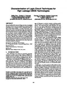
Server power supply (14%) Processor (15%) Fig. 1. 2. Energy demand in data centers [4]. $10 billion in electricity bills [3]. Moreover, 38% of the electricity is consumed for cooling the data centers as shown in Fig. 1. 2 [4]. That is, the energy efficiency becomes the utmost important factor even for maintaining data centers due to the cost and heat generated from its electricity consumption. Although the mainstream of electronics (i.e. CPU, Memory) has been improved exponentially owing to the rapid scaling down of silicon technology as shown in Fig. 1. 1, apparently wireline communication technology is relatively retarded because the communication channels (i.e. copper channel) is in fact placed out of the integrated ‘digital’ world but in the physical ‘analog’ world. That is the main reason for such a large portion of power consumptions by the high-speed input/output (I/O) circuits for wireline communications in modern computing systems. Technical breakthroughs are, therefore, highly demanded to enhance the energy efficiency of the high-speed I/Os. As shown in Fig. 1. 3, a general high-speed I/O link is composed of three main building blocks; a high-frequency clock generator, a serializing transmitter, and a 2

deserializing receiver. The clock generator produces a high-frequency clock from a low-frequency reference clock. The transmitter serializes parallel bitstream into a single bitstream by time-division multiplexing using the generated high-speed clock before sending the data. And the transmitter sends the serialized data through the properly impedance-matched transmission line. As long as the signal does not get reflected and does not cause interference, the high-speed I/O link can send the next signal even before the current signal reaches the receiver. In this way, the signaling rate is greatly enhanced without limited by the channel latency. In order to guarantee the proper impedance-matching, the transmitter should provide the fixed output impedance, which is same as the characteristic impedance of the transmission line. In the receiver side, the proper impedance matching is required also. Moreover, precise timing information is recovered for restoring the incoming time-multiplexed data, because adjacent bits are distinguished only by their positions in time. With the recovered timing information, sampling amplifiers are generally used to restore the incoming low-swing signal into the high-swing digital signal. And last, the receiver deserializes the recovered data into parallel bitstream. In this thesis, various circuit techniques for enhancing the efficiency of the clock generator, the serializing transmitter, and the receiver in CMOS technology are proposed. The proposed designs achieve much lower power and area consumptions compared to the state-of-the-art designs.

3

Data channel

RX Term.& Pre-amp

Clock & data recovery

Impedancematched Driver

Clock channel

RX Term. & Amp

CLK Gen.

Fig. 1. 3. Block diagram of general high-speed I/O transceiver.

4

Upper Link

High-speed I/O Receiver Deserializer

Serializer

Upper Link

High-speed I/O Transmitter

1.2. Thesis organization

This thesis is organized as follows. In Chapter 2, a design of a low-power and area-efficient high-frequency clock generator, which is based on a ring-oscillator based phase-locked loop, is presented. Circuit techniques including a two-stage ring oscillator, high-frequency clock buffer, and high-speed frequency divider are analyzed and verified. Moreover, structural design considerations for enhancing the energy efficiency of a high-speed I/O are introduced in Chapter 2. And last, the measurement results from a prototype chip fabricated in 65-nm CMOS technology are presented. Chapter 3 presents a design of an energy-efficient wide-range I/O transmitter. The proposed transmitter offers a wide operation range, controllable pre-emphasis equalization and output voltage swing without altering output impedance, and power supply scalability. Design considerations on a scalable wide-range transmitter are analyzed in Chapter 3. Based on the analysis, P-over-N multiplexing voltage-mode driver with two impedance calibrating regulators is used. Moreover, the circuit implementation and measurement results of a prototype chip fabricated in 65-nm CMOS are shown. In Chapter 4, a bit-error-rate (BER) analysis for a high-speed I/O link and a jitter tolerance analysis are presented. According to the analysis, a forwarded-clock (FC) receiver with a delay-locked loop (DLL) based de-skewing is employed in order to maximize the jitter tolerance while minimizing power and area consumption. Moreover, the stuck locking issue of the DLL-based FC receiver is addressed, and sample-swapping bang-bang phase detector (SS-BBPD) is proposed to eliminate 5

the stuck locking and to enhance the jitter tolerance with the minimal hardware overhead. The measurement results from a prototype chip fabricated in 65-nm CMOS technology are presented. Chapter 5 summarizes the proposed circuit techniques and concludes this thesis.

6

Chapter 2. Phase-Locked Loop Based on Two-Stage Ring Oscillator 2.1. Overivew In the data-driven world that we would be facing in the near future, there will be an explosive growth in the number of devices connected to a central system [1]. Inevitably, it would lead to a tremendous increase in the amount of digital data and communication bandwidth. Moreover, content-intensive video data will account for the highest portion of the digital data [1], and therefore, the rate of increase in the quantity of data will be much higher than the rate of increase in the number of devices. As a result, the required bandwidth of I/O transceivers supporting routers and server systems should be greatly improved in order to satisfy the increased demand. Nowadays, the per-pin bandwidth of the serial link transceivers fabricated in CMOS technology has reached 40 Gb/s in several reported designs [5]-[9]. The energy efficiency of the serial link transceiver is another important factor. The energy efficiency is 90 pJ/bit in the first 40-Gb/s– transceiver reported in [9], and has been improved to 23.2 pJ/bit in a recent design reported in [5]. However, there is still plenty of room for improvement, and therefore, circuits and architectures to improve energy efficiency are being continuously explored. Since data transmission in the serial link technology is based on time-division multiplexing [10], a phase-locked loop (PLL) which generates a high frequency clock from a reference clock is one of the most important building blocks of the 7

serial link transmitter. The PLLs in [5]-[9] employs high-Q LC tanks because of their high frequency. However, high-Q LC tanks are too costly in the fine-line digital CMOS technology [11]. On the other hand, as CMOS technology scales down, the performance of CMOS ring oscillators in terms of oscillation frequency and power consumption is further improved. In this work, the design of a PLL based on a ring oscillator, which provides clocking for a 40-Gb/s transmitter is presented along with an analysis on the optimal clocking architecture. A brief operating principle and performance summary of a ring oscillator is shown in Fig. 2. 1(a). The basic structure of a ring oscillator is a buffer array with negative feedback. For the feedback loop to sustain oscillations, the Barkhausen criteria should be satisfied; i.e., the overall loop delay should be 180 and the loop gain at the oscillation frequency should be larger than unity. The number of stages (N) is the most important parameter because the oscillation frequency, power consumption, and the Barkhausen criteria are directly related to N. Moreover, N determines the number of phases that a ring oscillator can generate since each buffer provides a clock output, whose phase is delayed over the preceding buffer output by a buffer delay. As long as the Barkhausen criteria and the number of phases generated are satisfied, a smaller value of N offers a better performance, as expressed in the performance summary in Fig. 1(a). In practice, a smaller N further improves the speed and power of the ring oscillator when we consider the parasitic capacitance of the routing wires. An example is shown in Fig. 1(b). Compared with an N-stage ring, an M-stage ring (N > M) has a smaller layout and fewer number of wires. Therefore, it has shorter routing wires and smaller parasitic capacitances, assuming both are implemented with the same buffer size. Then, the buffer size required to achieve the same frequency and the layout size are reduced, and thereby 8

the routing wires can be further shortened. That is, considering the practical layout issues, a smaller N provides faster speed and lower power consumption than that expected from the simple formulas. This chapter presents a PLL design that employs a ring oscillator with N reduced to 2 [12]. The design techniques for the PLL building blocks, including a ring oscillator, a clock buffer, a charge-pump, and a frequency divider, for a minimal power overhead are described.

9

t D, Astg

CL

t D, Astg

t D, Astg

CL

Barkhausen Criteria

Ring Performance

ÐHloop = NÐHstg(fosc) = -p,

fosc=1/(2NtD)

|Hloop| = |HstgN(fosc)| > 1

Posc=NCLVswing2fosc

(a)

N-stage Ring Buffer Cell

Buffer Cell

M-stage Ring Buffer Cell

Decreased Wire Parasitic

fosc,N=1/(2NtD,N) Posc,N=NCL,NVswing2fosc,N N>M CL,N>CL,M tD,N>tD,M

fosc,M=1/(2MtD,M) Posc,M=NCL,MVswing2fosc,M

Cell Size Reduced Further Decreased Wire Length

(b) Fig. 2. 1. (a) Barkhausen criteria and performance summary of a ring oscillator (b) layout consideration of a ring oscillator: reduction of the parasitic capacitance of routing wires

10

2.2. Background and Analysis of a Two-stage Ring Oscillator A. Optimal Clocking Architecture for a 40-Gb/s Serial Link Transmitter This section introduces the design considerations of the clocking architecture for a 40-Gb/s serial link transmitter. In the conventional serial link transmitter, signaling circuits such as output drivers consume a large portion of the transmitter power. However, as the data rate increases, the power consumed by inter-chip buffers also increases and surpasses the static power consumed by the output drivers, because the output drivers have the same 50- load regardless of the operating speed. Especially, the clock buffer, which delivers the fastest signal to the largest load in the transmitter chip, dissipates a large amount of power. Therefore, parallel-clocking architecture, which is optimized to minimize the inter-chip clocking overhead, enhances the energy and area efficiencies of the transmitter [13], [14]. A fanout-of-four (FO4) CMOS inverter-chain, which provides minimal delay and energy efficiency to drive a certain capacitive load, can be used as the clock buffer at low clock frequencies. However, due to the technology-defined circuit bandwidth, the FO4 inverter-chain suffers jitter amplification and duty-cycle distortion at frequencies higher than the FO4 bandwidth [15]. By reducing the fanout, the CMOS inverter-chain can operate at a higher frequency, but at the cost of energy efficiency and an increase in the delay. The power consumption of the CMOS inverter-chain, which drives a capacitive load of CL in Fig. 2. 2(b) is expressed as, 

C LVDD 2 fclk k   C LVDD 2 fclk , n k k -1 n 0

PCMOS  

11

(2.1)

VDD

VDD

R

R - Out +

In+

In-

CL

in

CL

out

IBIAS

CL

CML Buffer

CMOS Buffer

(a) Average Current

1st stage

(n-1)th stage

nth stage

CML

2pCLVswingfclk/kn-1

2pCLVswingfclk/k

2pCLVswingfclk

CMOS

CLVDDfclk/kn-1

CLVDDfclk/k

CLVDDfclk

CL/kn

Input

CL/k2

CL/k

CL k: fan-out (b) 100 Normalized Power Consumption

CMOS

CML

Overall CLK power

half-rate (1.0)

80

Half-rate 1.0 x 2 = 2.0

CML w/ reduced FO

60

CMOS w/ FO4

CMOS w/ reduced FO

40

CML w/ fixed FO

1/4th-rate (0.31)

20

1/8th-rate (0.11)

0 0

5 5G

10 10G

15 15G

20 20G

1/4th-rate 0.31 x 4 = 1.24 (38% improve over half-rate) 1/8th-rate 0.11 x 8 = 0.88 (56% improve over half-rate)

Clock Frequency (Hz)

(c) Fig. 2. 2. (a) Circuit diagrams of a CML buffer and a CMOS buffer (b) current consumption of the buffer chains (c) clocking analyses across the clock frequency

12

where k and fclk are the fanout of the inverter chain and the clock frequency, respectively, and the short-circuit current is neglected. Because a chain with too small a fanout can no longer be considered as a buffer and the power consumption of the chain increases dramatically as the fanout becomes closer to one [16], a fanout of two can be regarded as the speed limit of the CMOS inverter. To accommodate higher frequencies, a current-mode logic (CML) buffer that increases the circuit bandwidth by reducing the signal amplitude can be used. With the voltage swing (Vswing) and the circuit bandwidth of a CML buffer shown in Fig. 2. 2(a) being IBIASR and 1/(2pRC), respectively, the overall power consumption of the CML buffer chain can be expressed as 

PCML   n 0

2p C LVswingVDD fclk k

n



k  2p C LVswingVDD fclk , k -1

(2.2)

where it is assumed that the circuit bandwidth is the same as the clock frequency. Ideally, contrary to the CMOS buffer, the circuit bandwidth of the CML buffer is not a function of the fanout because R and IBIAS of the CML buffer are not technology-defined parameters. However, due to the limited current-density of a MOS transistor, the input device size is inversely proportional to R. That is, very small values of R require large input devices, and the resulting large gate and drain capacitances degrade the speed of the CML buffer chain [17]. As a result, the CML buffer also has to decrease the fanout to support higher frequencies, similar to the CMOS buffer. Based on the above analysis, the power consumption of the clock buffer over the clock frequency range is depicted in Fig. 2. 2(c). The upper limit of the operating frequency of the FO4 CMOS inverter and the one with a reduced fanout are decided based on the simulations using the 65-nm CMOS technology. Since too low a voltage swing results in low signal-to-noise ratio (SNR) and 13

requires a large input device size, which degrades the speed of the CML buffer chain [17], [22], Vswing is assumed to be one-fourth of VDD from the result shown in Fig. 2(c). Compared with the half-rate clocking utilizing the CML buffer, the quarter-rate clocking and the 1/8-rate clocking reduce the power consumption by 38% and 56%, respectively. In this work, quarter-rate clocking is chosen because the hardware complexity is doubled and also considering that power saving is not much improved in 1/8-rate clocking.

14

B. Models for a Two-Stage Ring Oscillator A quarter-rate 40-Gb/s transmitter requires a 90-spaced multi-phase 10-GHz clock. A four-stage ring oscillator is generally used to generate the 90-spaced multi-phase clock, but a two-stage differential ring oscillator, if it could be implemented as described in Section 2.1, would be a better option. Moreover, it is hard to build a four-stage ring oscillator operating at 10 GHz in the 65-nm CMOS technology. Therefore, a possible solution is to use a two-stage ring oscillator [18][21]. In our previous work [12], the implementation of a pseudo-differential twostage ring oscillator has been described. This section details the analytic model for a pseudo-differential two-stage ring oscillator. Actually, a two-stage ring oscillator is an extension of a four-stage, single-ended inverter-ring, as shown in Fig. 3. In general, the four-stage inverter-ring latches up, rather than oscillating, because the loop forms a positive feedback rather than a negative feedback near zero frequency because of signal inversion through each inverter [23]. However, in a special case, which provides proper initial conditions and a sufficient 90 phase shift in each stage, the ring oscillates and has an oscillation period of four inverter delays. By placing a sufficiently strong cross-coupled inverter pair between the diagonal nodes, the initial condition can be set, and the latch-up at DC can be resolved. Moreover, the cross-coupled pair tries to keep a 180 phase difference between the diagonal nodes, whose phases are apart by the two-stage inverter delay, so that it forces a 90 phase shift per stage which cannot be achieved in a conventional inverter model [23], [24]. The detailed phase-shifting mechanism of the pseudo-differential inverter is described in [12]. 15

Nominal Operation

Proper Initial Condition & 90 Phase Shift /Stage

Realization Using Cross-Coupled Latch

A=1

B=0

A

B

A=0

B=0

A=0

B=0

D=0

C=1

D

C

D=1

C=1

D=1

C=1

A B C

A Latch-up due to signal inversion at DC

B

2-stage differential ring oscillator

C

D

D

Latch keeps 180 phase between diagonal nodes 1. Prevent latch-up and set initial condition 2. 180 shift by 2 stage – 90 shift per stage

4td

Fig. 2. 3. Operating condition of a pseudo-differential two-stage ring oscillator and realization using cross-coupled latches. The waveform of a two-stage ring oscillator is slightly different from that of other ring oscillators. Compared with an LC oscillator, which exhibits sinusoidal waveform, the waveform of a ring oscillator is more likely to be a square wave because of the short transition time. The simplest model for the waveform of the ring oscillator is the first-order transition approximation; but it does not include the non-linear characteristics of the ring oscillators [25]. On the other hand, a secondorder model gives a more precise approximation. In [24], the second-order approximation is used to calculate the RMS value of the impulse-sensitivity function (ISF) of ring oscillators, and the results provided in [24] verify that the approximation is quite appropriate; however, it is hard to express the waveform in a closed form. Especially for a two-stage ring oscillator, the waveform can be approximated to be sinusoidal because it has a waveform whose transition time is relatively wide. Fig. 2. 4 shows the comparison of the approximated waveforms and the simulated waveform of a two-stage ring oscillator. The sinusoidal 16

Sinusoidal 2nd order 1st order Simulation

0

5

10

15

20

Fig. 2. 4. Waveform approximations for a two-stage ring oscillator. approximation matches well with the simulated waveform, as assumed in the analysis in [12].

17

C. Analysis on a Two-Stage Ring Oscillator In [12], the phase shift by a pseudo-differential inverter is analyzed, and the analysis verified using closed-loop transient simulations. This approach is based on the assumption that there are two elements introducing this phase shift: one is the RC time constant used in the conventional inverter model [26], and the other is the hysteresis by the cross-coupled inverter (hys), as shown in Fig. 2. 5(a). The result

1x

UG: Phase shift by RC time constant ax

1x

hys: Phase shift by hysteresis due to latch

(a) Oscillation Boundary

100

90º

Phase (º)

80

계열1 UG

60

계열2 hys

40

계열3 hys+UG

20 0 0

0.2

0.4

0.6

0.8

1

Latch ratio

(b) Fig. 2. 5. (a) Phase shift of a pseudo-differential inverter and (b) analysis result in [12]. 18

from the analysis is shown in Fig. 2. 5(b). The phase shift at the unity gain frequency (UG) cannot exceed 90, which is required to sustain oscillation. However, the phase shift by the hysteresis increases as the latch size increases, and therefore the overall phase shift exceeds 90 when the latch ratio is greater than 0.6. That means, the two-stage ring satisfies the Barkhausen criteria, when the latch size is sufficient. However, the Barkhausen criteria guarantee only the sustainability of oscillation, and not the start-up of oscillation [25]. The ring oscillator may have start-up failures according to the latch ratio and the initial conditions [25], [27]. Since the oscillation frequency and the probability of failures are decreased as the latch ratio is increased as shown in Fig. 2. 6(a), the latch ratio is one of the most important parameters in the design of a two-stage ring oscillator. To determine the latch ratio for a failure-free operation, start-up failure tests are carried out, using the SPICE transient analysis, across the 4-dimensional initial-condition space around a latch ratio of 0.6 and 0.7. The result shows that under the noiseless condition, the twostage ring with a latch ratio of 0.7 exhibits only 5 failure cases out of 28,561 initial conditions, while the ring with the latch ratio of 0.6 has 654 failure cases. As shown in the simplified graphical illustration in Fig. 2. 6(b), the two-stage ring with the latch ratio of 0.7 has a very narrow failure region, which indicates that such a condition can easily escape by small perturbations such as noises of devices [25]. Transient simulations with transistor noise are carried out for the 5 failure cases and the results, which are shown in Fig. 2. 7, verify that the ring escapes from the DC equilibrium points successfully. Since the transient simulation with the device noise requires a long simulation time, only a few select cases with the latch ratio of 0.6 are simulated. The result shows that the probability of failure is greater than 19

1.00 % even when the transistor noise is included. Moreover, when a failure test with a supply ramp as shown in Fig. 2. 6(a) is carried out, no failure is detected with the latch ratio of 0.7, whereas a failure probability of 0.85 % remains with the latch ratio of 0.6. Thus, the latch ratio of 0.7 is selected in order to guarantee the margin for oscillation while maximizing the oscillation frequency for the real implementation. The measurement results from a start-up test using the prototype chip will be presented in Section 2.4.

20

1 0.5

Probability of Failures 0

Frequency (GHz)

20

15 10 Keeper

Oscillator

Supply Ramp

5

VDD

0

0

0.2

0.4

0.6

0.8

0.1V

1

Latch Ratio(LR)

1ns

Latch ratio

Total # of I.C.

# of failures

Probability of failures

With Transistor Noise

0.6

28561

654

2.29 %

> 1.00 %

0.85 %

0.7

28561

5

0.017 %

0.00 %

0.00 %

With VDD Ramp

w/ Noise and Supply Ramp

2-Stage Ring Failure Simulation Results w/o Noise Across 4-Dimensional Initial Condition Space

(a) Initial Condition Space Failure Space for LR=0.7

Hard to escape with small perturbation

Escape with small perturbation

Failure Space for LR=0.6

(b) Fig. 2. 6. (a) Start-up failures of a two-stage ring oscillator by initial conditions and failure simulation results across the 4-dimensional initialcondition space (b) graphical illustration of the oscillation failures in 2dimensional initial-condition space. 21

1.2

1.2 Case #1

Case #2

0.9

0.9

0.6

0.6

0.3

0.3

0 0

0.2ns 2E-10 0.4ns 4E-10 0.6ns 6E-10 0.8ns 8E-10

1ns 1E-09

1.2

0 0

0.2ns 2E-10 0.4ns 4E-10 0.6ns 6E-10 0.8ns 8E-10

1ns 1E-09

1.2 Case #3

Case #4

0.9

0.9

0.6

0.6

0.3

0.3

0 0

0.2ns 2E-10 0.4ns 4E-10 0.6ns 6E-10 0.8ns 8E-10

1ns 1E-09

0 0

0.2ns 2E-10 0.4ns 4E-10 0.6ns 6E-10 0.8ns 8E-10

1ns 1E-09

1.2

w/ Noise

Case #5

0.9

w/o Noise 0.6

Transient Simulation Results of Failure Cases from LR=0.7 Including Transistor Noise

0.3 0 0

0.2ns 2E-10 0.4ns 4E-10 0.6ns 6E-10 0.8ns 8E-10

1ns 1E-09

Fig. 2. 7. Transient simulation results of the 5 start-up failure cases from the latch ratio of 0.7 including noise of transistors. For a single-ended ring oscillator with sufficient symmetry, the phase noise is not a function of the number of stages [24], [28]-[30]. Because the two-stage pseudo-differential ring oscillator is an extension of the four-stage single-ended ring oscillator, the phase noise of the two-stage ring is well expected from the theories developed by Hajimiri and Lee [24] and by Abidi [28]. However, as described in the previous paragraph, the two-stage ring oscillator has a large crosscoupled latch as compared with other ring oscillators and therefore, the phase-noise contribution of the latch should be considered. A circuit diagram of a single-stage buffer in a two-stage ring oscillator, and the nodal waveforms in the buffer are shown in Fig. 2. 8(a) and Fig. 2. 8(b), respectively. Sinusoidal waveforms are assumed. The current that flows in the main buffer NMOS transistor (N1) and in 22

the latch NMOS transistor (N2) is shown in Fig. 2. 8(b). Because the gate and drain voltage phases of N2 (c90 and c270 in Fig. 2. 8(b)) are 180 apart, no current flows through N2 when its gate-overdrive voltage is at the maximum and it hardly operates in saturation region. On the other hand, a large current flows through N1 when its gate voltage (c0) is at VDD, because the drain voltage (c270) is VDD/2 at that time. Moreover, N2 is turned on when the ISF of the output is relatively low, whereas N1 is turned on when the ISF has the maximum amplitude. That is, compared with the main buffer, the latch injects much less noise current and the injection occurs when the ISF is at the minimum. The ratio of the simulated phasenoise contribution by the latch to that by the main buffer is shown in Fig. 2. 8(c). The latch contribution to the phase-noise is 14 dB less than the main buffer contribution when the latch ratio is 0.7, which implies that the effect of the latch could be neglected in the phase-noise analysis.

23

Main buffer

Latch

c270

c0 N1

Main buffer

c180

c90 N2

(a) VDD c270

c0

c90 0 I(N1) Latch flows much less current

I(N2)

ISF (c270)

0 N2 noise affects @ small ISF region

N1 noise affects @ large ISF region

(b)

PN(Latch) / PN(Main)

Latch ratio -10 0.5

0.6

0.7

0.8

0.9

0.6

0.7

0.8

0.9

1

-11 -12 -13 -14 -15 -16

(c) Fig. 2. 8 (a) Circuit diagram of a pseudo-differential inverter (b) qualitative comparison between phase-noise contributions of the main buffer and the latch (c) simulated phase noise contribution ratio. 24

2.3. Circuit Implementation of The Proposed PLL

The overall block diagram of the proposed PLL is shown in Fig. 2. 9. A charge pump with a replica-feedback bias is used, and its current is adjusted to control the PLL loop bandwidth [31]. A voltage-controlled oscillator (VCO) based on a twostage ring oscillator generates a 90-spaced four-phase clock. Coarse frequency selection is used in the ring-VCO to support a wide-range operation and to accommodate the process, voltage, and temperature (PVT) variations. The overall division factor of the PLL is 16, and the first divider is implemented with the tristate-inverter–based divider which can operate at the maximum frequency that the VCO can generate— which is much higher than 10 GHz. An AC-coupled clock buffer corrects the common level and duty-cycle of the VCO output and the clock is buffered to the data lanes [12]. The phase-frequency detector (PFD) is implemented as described in [32]. Fig. 2. 10 shows the circuit diagram of the VCO. A latch ratio of 0.7 is used

Loop BW control

Coarse freq. band selection

up REF down

/4

4

CP/ LF

PFD

ACcoupled buffer

2-stage ring VCO /2

/2

TSPC divider

Tri-inv. based divider

4

CLK To TXs

CLK Buffer

Fig. 2. 9. Block diagram of the PLL. 25

1x 0.7x 1x

Coarse Control

Vctrl

Fig. 2. 10. Circuit diagram of the implemented two-stage ring oscillator.

# of MC Samples

200

 = 1.22%

160

(0.305 ps) 120

80 40

-4.75 -4.25 -3.75 -3.25 -2.75 -2.25 -1.75 -1.25 -0.75 -0.25 0.25 0.75 1.25 1.75 2.25 2.75 3.25 3.75 4.25 4.75

0 -4%

-2%

-0%

2%

4%

I/Q Mismatch

Fig. 2. 11. Simulated I/Q phase mismatch of the two-stage ring VCO.

according to the analysis described in Section 2. C. The simulated I/Q phasemismatch of the two-stage ring VCO from 1000 Monte Carlo samples is shown in Fig. 2. 11. Since the I/Q phase-mismatch introduces a duty-cycle error, which degrades the timing margin of the transmitted signal of the quarter-rate transmitter, the VCO is designed to have an I/Q mismatch less than 1 ps within a 3 range. On the other hand, to maximize the speed by reducing the voltage dropout by the control device, a current-starved ring oscillator that has only a pull-down current 26

source at the bottom of the NMOS devices is used. However, the output common level of the VCO is not constant across the tuning range and PVT variations, because it is a function of the current that the control-device draws. When the current increases, the capacitors at the oscillation nodes are charged or discharged faster so that the oscillation frequency increases. However, the required gateoverdrive voltages of the devices in the inverter also increase to draw the increased current, which causes the common level at the oscillation nodes to decrease. The AC-coupled clock-buffers shown in Fig. 2. 12(a) are used to reject the commonlevel variation and duty-cycle distortion. The resistive feedback offers self-biasing and bandwidth extension. The approximate small-signal transfer function of the AC-coupled inverter with a resistive feedback is expressed as

vo sgm RF CC , RF CC 1 vin 2 gm   s(C L  CC  )  s RF CC C L ro ro

27

(2.3)

RF=26k CL

CC=17f vin from VCO

1u/2u

vx

Duty/Common Correction

-AF

vout

Gain Stage

(a) 20 700M

Gain (dB)

10

15G

-3dB

0 -10 -20 -30 -40 -50 1M 1

10M 1G 10000100000 10G 100G 10 100M 100 1000

Frequency (Hz) (b) Fig. 2. 12. (a) Circuit diagram and (b) transfer function of the VCO clock buffer where RF is the feedback resistance, CC is the AC-coupling capacitance, and ro and CL are the small-signal output impedance of the inverter and the load capacitance at the output of the AC-coupled inverter (vx), respectively. gm is the trans-conductance of the inverter, which is assumed to be much larger than 1/RF. From (2.3), we can find that the AC-coupled inverter with a resistive feedback is a kind of bandpass filter, and the simulated high-pass and the low-pass cut-off frequencies are 700 MHz and 15 GHz, respectively, as shown in the transfer function in Fig. 2. 12(b). Because the high-pass cut-off frequency is relatively high; a metal-oxide-metal (MOM) capacitor (which uses the metal layers from metal3 to metal6) with a very small area of 2.5 × 4.5 m2 and a small parasitic capacitance of less than 2 fF is 28

clk

clk

clk

Large fanout

clk

Fig. 2. 13. Circuit diagram of a TSPC divider. used. A post-layout simulation shows that each VCO clock buffer dissipates 160 μW. Along with the VCO, a frequency divider is the other building block operating at the highest frequency in the PLL. Moreover, the frequency divider should cover the wide frequency range from the minimum to the maximum frequency that the VCO can generate, in order to avoid a global convergence failure [27]. Among the conventional CMOS-logic-based frequency dividers, a true-single-phase-clock (TSPC) frequency divider shown in Fig. 13 exhibits the highest operating frequency. However, considering an output buffer, the stacked MOS devices face a large fanout at the output node of the TSPC divider, and therefore, the maximum frequency that the divider can endure is limited. To build a frequency divider operating at a higher frequency in CMOS-logic circuits, a tri-state inverter is used as a latch to minimize the feedback delay as shown in Fig. 2. 14(a). Because only a tri-state inverter is transparent at once, the two cascaded tri-state inverters act as a flip-flop, and the divider has a loop delay of three gate delays. Since the output node is driven by the non-stacked CMOS inverter so that the logical effort is not sacrificed, the tri-state-inverter–based divider can cover higher frequencies than the 29

TSPC divider. A post-layout simulation in Fig. 2. 14(b) shows that the tri-stateinverter–based divider operates well up to 20 GHz. The divider has a drawback that the output duty-cycle is susceptible to the duty-cycle error of the input differential clock, but it does not affect the PLL performance because the succeeding dividers eliminate the duty-cycle error of the first divider. The circuit diagram of the charge pump is shown in the Fig. 2. 15(a). The charge pump reduces both the up/down current-mismatch and variation, using the dualcompensation loop based on replica-feedback biasing [31]. The charge-pump is segmented for the coarse tuning of the PLL loop bandwidth. The reference voltage (vn1 in Fig. 2. 15 a)) of the replica-feedback biasing circuit is adjustable for finetuning. Simulated charge-pump currents across the output voltage range with the nominal setting are shown in Fig. 2. 15(b). The charge-pump exhibits nearly zero current-mismatch and variation across a wide range of output voltages.

30

Tri-state inverter based flipflop

clk

clkb A

clkb

clk

out clk clkb A

Pass

out

Hold

Hold

Pass

Pass

Hold

Hold

Pass

(a) 250

Power (uW)

200

TSPC

Tri-inv

150 100 50 0 0

5

10

15

20

25

Frequency (GHz)

(b) Fig. 2. 14. (a) Circuit diagram of the tri-state-inverter–based divider and (b) comparison with the TSPC divider.

31

Segmentation for Coarse Tuning

Adjustable vn1 for Fine Tuning I1

vp2

I2

vp1

up

vp2

I1

vp1

up

I2

vp2

vctrl

vctrl

vctrl vn1

vn1

vn2

vn1

dn

Replica-Feedback Bias Circuit

vn2

I1

dn

I2

Charge Pump Segment

Pump Current (uA)

(a)

40 30

Pull-down 20

Pull-up 10 0 0

0.3 0.3

0.6 0.6

0.9 0.9

1.2 1.2

vctrl (V)

(b) Fig. 2. 15. (a) Circuit diagram of the charge-pump with replica-feedback bias and (b) simulated pump currents across the output voltages.

32

2.4. Measurement Results The prototype chip has been fabricated in the 65-nm CMOS technology. The die photomicrograph and block description are shown in Fig. 2. 16. One of the transmitter lanes is dedicated to measure the PLL clock. The proposed PLL for a 40-Gb/s serial link transmitter occupies an active area of 0.009 mm2, including the loop filter. The die is wire-bonded on a four-layer RO-4350B printed circuit board (PCB). To verify the start-up failure issue of the two-stage ring oscillator, a powerup test is carried out. No failure is detected in 1000 repetitions of the power-up test. Owing to the wide tuning range of the two-state ring VCO, the proposed PLL operates within a wide frequency range from 1.25 GHz to 10 GHz. The measured eye diagrams of the PLL clock over the operating frequency range are shown in Fig. 2. 17. The measured power dissipation of the overall clock-domain, which includes the PLL and the clock buffers driving the multi-phase clock from the PLL to each data lane, is 27.6 mW from a 1.2-V supply at 10 GHz. Most of the power is

CH0

PRBS Gen. PLL

CH1

90u

0.48mm

consumed in the clock buffer and the power consumption of the PLL is 7.6 mW.

100u

0.36mm

Fig. 2. 16. Die photomicrograph. 33

10 GHz

7 GHz

50 ps

50ps

2.5 GHz

1.25 GHz

100ps

400ps

Fig. 2. 17. Measured eye diagrams of the PLL clock across the operating frequency range. The measured phase noise, integrated RMS jitter from 10 kHz to 100 MHz, and the reference spur are shown in Fig. 2. 18 and Fig. 2. 19. Agilent E4445A Spectrum Analyzer is used to measure the phase noise and Agilent N4903 J-BERT is used to provide the reference clock. The measured reference spur and integrated RMS jitter are -58.28 dBc and 414 fs, respectively, at 10 GHz. The sub-harmonic spurs are due to the capacitive coupling between the loop filter and the additional frequency dividers for measurement. From the measured integrated jitter and the power consumption, the following figure-of-merit (FoM) can be calculated as 2      P    FoM J  10log  t   DC   ,   1s   1mW   

(2.4)

where t and PDC are the integrated RMS jitter and the average power consumption, respectively. The resulting FoMJ of the proposed PLL is -238.8 dB. The performance of the proposed PLL is compared with that of the recently published 34

Free-running VCO (sim)

Phase Noise (dBc/Hz)

-50 -60 -60 -70

Integrated Jitter: 414 fs(10k-100M) 7.6mW from 1.2V VDD

PLL

-80 -80 -90 -100 -100

REF

-110 -120 -120 -130 -140 -140 -150 1000

1k

10000

10k

100000 100k

1000000

1M

10000000

10M

100000000

100M

Frequency Offset (Hz)

Fig. 2. 18. Measured phase noise and integrated RMS jitter

Ref. Spur -58.28 dB

625MHz

Fig. 2. 19. Measured frequency spectrum and reference spur of the PLL at 10 GHz. state-of-the-art PLLs using ring oscillators, in terms of the jitter performance and energy cost in Fig. 2. 20. Ring-PLL designs whose maximum achievable frequencies are higher than 2 GHz are included in Fig. 2. 20 [18], [33]-[42]. The proposed PLL is at the second in terms of energy cost and on top in terms of FoMJ. For the integer-N ring PLLs in [33]-[37], a more detailed performance comparison is summarized in the Table 2. 1.

35

JRMS2 x Freq. (ps2 x GHz)

Integer-N Fo M Fo M

10

Fo M

-2

Fo M 34

-2

dB

37

-2 4

-2 3

Fo M 1d B

Fractional-N -2 2

-2 2

Huang, isscc’14 Xiu, jssc’13

5d B

8d B

Liang, isscc’15 Nandwana, jssc’15

dB

Chiang, asscc’15

Jang, tcasII’15 Tsai, isscc’15 Yang, tcasII’14

0d B

Lee, cicc’15 Cho, esscirc’15 Chien, isscc’14

This work

1 0.1

1

10

Power/Freq. (mW/GHz) Fig. 2. 20. Jitter performance versus energy cost comparison for ring-PLLs.

Table 2. 1. Performance comparison of the proposed PLL ISSCC '14 [33]

TCAS-II '14 [34]

ESSCIRC '15 [35]

CICC '15 [36]

ASSCC '15 [37]

This work

Frequency

15 GHz

6 GHz

5 GHz

2 GHz

5 GHz

10 GHz

Ref. Clk

1.875 GHz

375 MHz

156.25 MHz

125 MHz

250 MHz

625 MHz

Power (mW)

46.2

11.6*

15.4

3.74

3.34

7.6

Technology

20 nm

90 nm

65 nm

65 nm

40 nm

65 nm

Supply (V)

1.25/1.0

1.0

1.2

0.9

1.1

1.2

Area (mm2)

0.044

0.4

0.06

0.1

0.0049

0.009

Ref. Spur

-48 dBc

N/A

-42.61 dBc

-48 dBc

-51.06 dBc

-58.28 dBc

RMS Jitter

268 fs

828 fs

484 fs

971 fs

1.242 ps

414 fs

FOMJ (dB)

-234.8

-231.0

-234.4

-234.5

-232.9

-238.8

36

Chapter 3. A Scalable Voltage-Mode Transmitter 3.1. Overview Multi-standard serial link transceiver offers flexibilities in designing a system on a chip. As shown in Fig. 3. 1, although only a single I/O standard is considered, some famous standards such as Universal Serial Bus (USB), Serial ATA (SATA), and Peripheral Component Interconnect Express (PCIe) require a backward compatibility so that the wide-range operation should be included in their implementations. A serial link transmitter should provide a fixed output impedance, a pre-emphasis equalization and a controllable output swing without altering the output impedance [43]. Moreover, to support multiple standards and to maximize the energy efficiency, the transmitter should have a wide operating frequency range and supply voltage scalability [44]. Although the state-of-the-art designs, which exhibit the best energy efficiency, adopted a scalable supply design, provided externally, not from internal supply regulators or DC-DC converters [44]-[47]. Voltage-mode (VM) driver is preferred in many recent low-power wireline transmitter designs, where only one-fourth current of a current mode (CM) driver is dissipated [43], [45]-[50]. However, still the CM drivers are in the mainstream for the transmitter operating at the speed of higher than 20 Gb/s [5], [51]-[54], because the VM drivers suffer from several challenges at the high speed era, for instance, difficulties in implementing equalization, huge power consumption in the pre37

Data rate (Gb/s)

16G

16 10G

4

6.0G

5.0G

3.0G

8.0G 5.0G 2.5G

1.5G

1 0.48G

0.25 2000USB3.1 2004SATA3.02008PCIe4.02012 Fig. 3. 1. Per-pin I/O bandwidth range required for some serial link standards. driver stages, and the non-linearity of the output impedance [16]. In fact in [16], a hybrid type driver utilizing constant Gm circuit to overcome the drawbacks of the conventional drivers has been proposed, yet with a limited output swing range. Clock generation circuit introduces several issues on designing a wide-range transceiver. Especially, to cover a wide range of frequency, the clock generation circuit consumes a lot of resources. Because an LC oscillator has a higher operating frequency but narrow frequency range, while a ring oscillator has a wider frequency range but lower operating frequency, a single phase-locked loop (PLL) with a single oscillator is hard to cover the wide frequency range. Therefore, most of the wide-range transceiver designs employ multiple PLLs, or oscillators [13], [52], [55]-[57]. In this work, a voltage-mode (VM) transmitter which offers a controllable output swing and pre-emphasis as well as the scalable supply, while matching the output impedance, is presented. This chapter discusses the design issues of a wide-range, 38

scalable transmitter from the perspectives of the I/O signaling circuits, inter-chip circuit topology, and architecture. Based on the analysis, a quarter-rate transmitter with a multiplexing P-over-N VM driver and a single ring-PLL is proposed.

39

3.2. Design Considerations on a Scalable Serial Link Transmitter This section describes the design considerations on a scalable multi-standard transmitter. One of the most important decisions that a designer should make is that which base circuit topology should be used in the transmitter chip, which is closely related to the clocking architecture. CMOS logic and current mode logic (CML) are two main circuit topologies in modern silicon technology. The CML circuits exhibit higher speed than the CMOS counterpart, but they can be power hungry because they dissipate static power, whereas the CMOS circuits dissipate only dynamic power. As the rule of thumb for CML circuits, the differential output amplitude should be at least 400 mVpp for proper operation, so the minimal power dissipation of a basic CML buffer depicted in Fig. 3. 2 becomes PCML  VDD I BIAS  VDD

200mV . R

(3.1)

Because the bandwidth of the CML buffer in frequency is 1/2p(RCL), (3.1)

VDD R

VDD R

- Out + In+

In-

CL

CL

in

out

IBIAS

CL

CML Buffer

CMOS Buffer

Fig. 3. 2. Circuit diagrams of basic CML and CMOS buffers 40

Power Consumption

30 25 CML, 20-GHz

20 15

CML, 10-GHz

10 CMOS

5 0 0

5G 5

10G 10

15G 15

20G 20

Frequency (Hz)

(a)

Power Efficiency

15 CML, 20-GHz

12 CML, 10-GHz

9 CMOS

6 3 0 0

5G 5

10G 10

15G 15

20G 20

Frequency (Hz)

(b) Fig. 3. 3. (a) Power consumptions by CML and CMOS buffers (b) power efficiency of CML and CMOS buffers. becomes PCML  2p VDDC L f BW  200 mV .

(3.2)

where fBW is the 3-dB bandwidth of the CML buffer. On the other hand, the maximal dynamic power consumed by the CMOS buffer described in Fig. 3. 3(a) is

PCMOS  CLVDD 2 fclk ,

(3.3)

where fclk is the clock frequency, when the short-circuit current is neglected. In general, the circuit bandwidths of a CML buffer and a CMOS buffer are not adaptable across the wide frequency range, because they are decided by the passive 41

RC time constant and by the fan-out from the buffer to the load capacitance and the device parameters given in the process, respectively. For the given fan-out and technology limits, the CMOS buffer has a certain bandwidth limitation whereas the CML buffer has more flexibility by designing a load resistance. Fig. 3. 3(a) shows PCMOS and PCML from (3.2) and (3.3) with the CML buffers designed to support up to 10 GHz and 20 GHz. The bandwidth limit of the CMOS buffer and the value of VDD are assumed to be 10 GHz and 1.0 V, respectively. Note that PCML in (3.2) is the minimal power dissipation by the CML buffer, because the minimal output amplitude of 400 mVpp is assumed. Although the CML buffer can achieve higher bandwidth, the power consumption is higher than that of the CMOS buffer, and is constant regardless of the operating frequency. The resulting power efficiency across the frequency is shown in Fig. 3. 3(b). The power efficiency of the CML buffer is severely degraded at the lower frequency while that of the CMOS buffer keeps constant at all frequencies. This means that to build an energy-efficient transmitter across a wide-range operation, the system should consist of CMOS based circuit. Generally, the fastest signal in a chip is a clock signal. As a result, determining the clocking architecture of a transmitter is related to the base circuit topology. As shown in Fig. 3. 4, parallel clocking structure, such as a half-rate or a quarter-rate clocking, in return for the increased hardware complexity, offers lower clock frequency and relaxes the required circuit bandwidth [13], [14]. As a result, the main aspects that should be considered while building an energy-efficient wide range transmitter can be summarized as follows. First of all, the maximal clock frequency in the transmitter should be chosen such that the CMOS buffer can support. Then, decide the degree of parallelism according to the maximal clock frequency. 42

Overall Power, Area Efficiency

Optimum Circuit BW Overload CMOS based design Hardware Complexity

Increasing parallelism

Increasing clock freq.

Fig. 3. 4. System power and area efficiency with respect to the parallelism and the clock frequency. Another important decision is the type of the signaling circuit, output driver. An output driver should provide a proper termination for signal integrity and a sufficient output swing to guarantee a sufficient signal-to-noise ratio (SNR). As described in section 3. 1, CM driver is preferred in high-speed transmitters, but it dissipates much more power than the VM driver does. Moreover, CM driver is less compatible with the CMOS buffer stage, and therefore CML buffers are required in the pre-driver stage, which makes it less attractive in the wide-range transmitter design. On the other hand, VM driver is compatible with the CMOS buffers because it uses active MOS devices as a switch which has a finite resistance. Fig. 3. 5(a) shows simplified circuit diagrams of the two main VM driver structures, Nover-N VM driver and P-over-N VM driver. With the differential configuration and the proper termination, the output differential peak-to-peak voltage swing of the both VM drivers is Vswing. Assuming that the input has the rail-to-rail CMOS level swing, the N-over-N VM driver exhibits impedance linearity with relatively small output swing, while the impedance of the P-over-N is linear with higher output swing, as shown in Fig. 3. 5(b) [48]. As well as exhibiting a wider linear range, the 43

P-over-N structure is more suitable for various serial I/O standards such as USB or PCIe, because they require differential transmitter voltage swing larger than 1.0 Vpp. In addition, an impedance calibration scheme should be included in the transmitter to provide a variable voltage swing without altering output impedance, because the active CMOS devices rather than passive resistors are used as termination resistors in a VM driver. Moreover, a pre-emphasis equalization to compensate the channel loss should be available and also adjustable to support the operation range exceeding 20 Gb/s.

44

Vswing

Vswing

in-

MP

MN2 out

in+

out

in MN3

MN1

P-over-N

N-over-N

Output Impedance ( )

(a)

P-over-N

300 300

N-over-N

200 200 Linear region

Linear region

100 100 0 0

0.5 0.5

1.0 1

Output Swing (Vdiff,pp) (b) Fig. 3. 5. (a) Simplified circuit diagrams and (b) simulated output impedances across the output swing range of N-over-N and P-over-N VM drivers.

45

3.3. Circuit Implementation A. Overall Architecture Fig. 3. 6 shows the overall architecture of the proposed wide-range scalable transmitter. To maximize the power efficiency and scalability while operating up to 32 Gb/s, a quarter-rate clocking architecture is employed since the maximal achievable speed of the CMOS buffer locates around 10 GHz in the 65-nm CMOS process. Moreover, the final 4:1 serializer is merged into the output driver to relax the circuit bandwidth of the pre-driver. The output driver is based on a P-over-N VM driver with impedance calibrating supply regulators. The output impedances of the pull-up PMOS devices and pull-down NMOS devices are controlled by the VDDPU regulator and the VDDPD regulator, respectively, because the NMOSs and HVDD (1.5V) Iref

Rint

+ _

+ _

MPD

+ _

Rint

Pull-Up Replica

MPU

VDDPU CH 1

Rref

Rref Segment Selection Pull-Down Replica

Serializer

2-stage ring PLL

RCM

Pre-emp. Selection

CH 1 CH 0

VDDCLK (1.1V)

RCM

CH 0 Segment Selection D clk180

VDDPD Domain

clk270 clk90

4

D 4 Buffered clocks

Pre-Driver

4

QDLL

clk0/90/180/270

CLK Buffer

clk0 D

Multiplexed VM Driver I/Q Phase Calibration

Fig. 3. 6. Circuit diagrams of basic CML and CMOS buffers 46

Simulated PSR (dB)

0 -10 VDDPD

-20 -30 VDDPU

-40

1k 1

100k 100

10M 10000

1G 1000000

Frequency (Hz) Fig. 3. 7. Simulated power supply rejections of the VDDPD regulator and VDDPU regulator. PMOSs are turned on when the input is logical high (VDDPD) and logical zero (0V), respectively. The regulators use the replicas of the pull-up and pull-down devices and the off-chip reference resistors to calibrate the output impedances. The numbers of the output driver segments and the replica segments included in the feedback loop are designed to be selectable. When the numbers of the activated segments are changed, the regulators adjust the VDDPU and VDDPD to match the impedances of the VM driver and the reference resistance. Therefore, the proposed transmitter can scale with the supply voltage and the output swing without disturbing the output impedance. Another advantage that the regulators offer is power supply rejection (PSR). The PSR of a linear regulator is expressed as, Vreg ( s ) VDD ( s )



r

load

/ ( rload  rpass ) (1  s / amp )

(1  s / reg )(1  s / amp )  Aamp Apass

.

(3.4)

where rpass is the output resistance of the pass gate (MPD and MPU in Fig. 3. 6), amp is the pole of the amplifier, reg is the pole at Vreg, Aamp is the gain of the amplifier, and Apass is the gain of the pass gate [58]. The dominant poles of both regulators are 47

placed at the output of the amplifier to avoid using the large capacitors. The simulated PSR of the regulators are shown in Fig. 3. 7. The regulators use one-fifth sized replicas of the devices in the driver, and the resulting impedance mismatches achieved from 1000 Monte-Carlo simulations are shown in Fig. 3. 8. The simulated standard deviation of the impedance mismatches are less than 0.7 % for both regulators. A 2-stage ring voltage-controlled oscillator (VCO) is used in the phase-locked loop (PLL) to generate a quarter-rate, 4-phase clock and to support a wide frequency range [12]. The pre-driver comprised of CMOS buffer arrays drives the 4-bit parallel data and the 4-phase clock to the output driver. The transmitter consists of two lanes, one of which is dedicated to measure the quarter-rate clock (1100 pattern), which has the same transition density as the full-rate random data. The regulators and PLL are shared among the channels. The regulators generate VDDPD and VDDPU from a 1.5-V supply, and the PLL uses an independent 1.1-V supply to decouple the high frequency switching noise and to shield the ring-VCO from the supply scaling.

48

250 200 200 150

 = 0.69%

NMOS VDDPD

100 100

2.2%

1.8%

1.4%

1.0%

0.2%

-0.2%

-0.6%

-1.0%

-1.4%

-1.8%

-2.2%

0 -2.4% -1.6% -0.8% 0%

0.6%

50 0.8% 1.6% 2.4%

Mismatch between driver&replica (a) 300 300 250 200 200

 = 0.63%

PMOS VDDPU

150 100 100

2.2%

1.8%

1.4%

1.0%

0.2%

-0.2%

-0.6%

-1.0%

-1.4%

-1.8%

-2.2%

0 -2.4% -1.6% -0.8% 0%

0.6%

50 0.8% 1.6% 2.4%

Mismatch between driver&replica (b) Fig. 3. 8. Simulated impedance mismatches between the driver and (a) NMOS replica in the VDDPD regulator (b) PMOS replica in the VDDPU regulator

49

B. Voltage-Mode Driver Fig. 8 shows the circuit and timing diagram of the proposed multiplexing VM driver. The multiplexing function is merged into the driver by stacking the datadriven devices and the clocked devices. The pre-emphasis implementation is based on a resistive divider in order to guarantee a constant output impedance across the pre-emphasis coefficient range [13]. The main tap and pre-emphasis tap are sliced to adjust the output swing and pre-emphasis coefficients, and their segments are implemented with exactly the same circuit. The pre-emphasis coefficient is tunable without altering the output impedance, because the output impedance is inversely proportional to the number of the overall activated slices regardless of whether the slices belong to the main tap, or the pre-emphasis tap. Each slice contains eight branches, each of which consists of triple-stacked NMOS, or PMOS devices. The branches are turned on one at a time, as shown in the timing diagram in Fig. 8. To minimize the transition delay, the clocks triggered last is placed at the closest devices to the output. The D3-D0 are retimed in the pre-driver stage by clk270, clk0, clk90, and clk180, respectively, to maximize the timing margin for the final 4:1 multiplexing as shown in the timing diagram in Fig. 3. 9. As described in section 3.3.A, when the number of activated slices is increased, the VDDPU regulator decreases VDDPU to maintain the constant output impedance. Therefore, the output voltage swing is adjustable by changing the number of the activated slices in the driver and replicas of the regulator.

50

clk0

Main Slices clk90

D0

clk180

clk270

clk0

clk270

clk0

clk90

D3

D2

D1

clk90

clk180

clk180

clk270

D3

M P

M P

D2

clk0

clk90

clk180

clk270

clk270

clk0

clk90

clk180

D1

D3

D2

D1

D0

D0

out

out D0 D3 D2 D1 D0 D3 D2 D1 D0 D3

Pre-emphasis Slices VDDPU controls voltage swing Segment VDD PU D0

D3

D2

D1

clk90

clk180

clk270

clk0

clk180

clk270

clk0

clk90

clk0

clk90

clk180

clk270

clk270

clk0

clk90

clk180

D0

D3

D2

D1

Rpre

Rmain

out

Rpre

Rpre

Rmain

out

Rmain

1 after 1

Rpre

Rmain

1 after 0

Fig. 3. 9. Circuit and timing diagrams of the proposed multiplexing voltagemode driver and the pre-emphasis principle.

51

C. Pre-Driver Fig. 3. 10 shows the implementation of the pre-driver stage. The driver segments selection logic is embedded at the first stage of the pre-driver to minimize the power and area overheads. The CMOS inverter array whose fan-out is two is used to drive a large input capacitance of the output driver up to 8 GHz. Because the proposed transmitter employs the quarter-rate clocking and the final 4:1 multilexing merged into the output driver, I/Q phase mismatch can severly degrade the timing margin. The simulated I/Q phase mismatch at 7-GHz clock frequency is shown in Fig. 3. 11. The standard deviation from the simulation is 2.57 %, which corresponds to 0.92 ps. To compensate the I/Q phase mismatch, a quadrature delaylocked loop (QDLL) proposed in [59] is used. While the quadrature phase detector compares the buffered clocks at the final output of the pre-driver, the voltagecontrolled delay line (VCDL) of the QDLL is placed before the pre-driver buffer array to minimize the VCDL power and size. The VCDL is designed to cover I/Q mismatch of at least 3- range. Simulated I/Q phase error transfer of the pre-driver with, or without QDLL is shown in Fig. 3. 12.

52

Main Driver PMOS Network (N Slices)

sel sel clk /D

clk0,90,270,360 D

Main Driver NMOS Network (N Slices)

sel sel clk /D

clk0,90,270,360 D

Pre-emph. Driver PMOS Network (M Slices)

sel_pe sel clk /D

clk90,270,360,0 D

Pre-emph. Driver NMOS Network (M Slices)

sel_pe sel clk /D

clk90,270,360,0 D

Fig. 3. 10. Implementation of the pre-driver. 200

 = 2.57%

150

(0.92 ps)

100 50 50

0 -9.5-8% -7.5 -5.5-4% -3.5 -1.5-0% 0.5 2.5 4% 4.5 6.5 8% 8.5

I/Q Mismatch Fig. 3. 11. Simulated I/Q phase mismatches at 7 GHz.

53

out (ps) 6 4 2 -4ps -6

-4

0 -2

0

2

-2

4ps 4

in 6

w/o QDLL

-4

w/ QDLL

-6

Fig. 3. 12. Simulated I/Q phase error transfer.

54

D. Phase-Locked Loop Recent wide-range transmitters use multiple oscillators to cover the wide frequency range. Because an LC oscillator has a narrow frequency range while a ring oscillator has a low maximal frequency, four LC oscillators are used in [56], and two LC oscillators for high-frequency and a ring oscillator per channel for low frequency are used in [57]. In this work, a single PLL, which maximizes the speed by using the optimized two-stage ring oscillator, covers the entire frequency range of 1.5-to-8 GHz with the assistance of the quarter-rate transmitter architecture. The details of the PLL are described in Chapter 2.

55

3.4. Measurement Results The proposed transmitter is fabricated in the 65-nm CMOS technology. In order to demonstrate the scalable voltage swing of the proposed transmitter, measured eye diagrams across the variable output swing are shown in Fig. 3. 13. The measurement was done at 16 Gb/s and the measured power consumption is from 33.7 mW/ch to 60.7 mW/ch across 250-to-600-mV single-ended swing range. The 250-mV and 300-mV swings are obtained from the low-power mode, which reduces the power consumption of the output driver by increasing the output impedance. Power consumption from the maximized pre-emphasis with the middle-level swing, whose eye diagram is depicted at the bottom-right of Fig. 3. 13,

250mV, 33.7mW/ch

600mV, 60.7mW/ch

160mV

Energy Efficiency (pJ/bit)

500mV, 57.7mW/ch

300mV, 38.2mW/ch

75mV

75mV

400mV, 47.2mW/ch

160mV

400mV w/ PE, 53.9mW/ch

75mV

75mV

5 4 3

2.95 2.10

3.60 3.79 3.37

2.38

2 1 0 250 250

300 400 400 500 600 600 400 300 500 w/ PE Output Swing (mV)

Fig. 3. 13. Eye diagrams and energy efficiencies across the output swing range at 16 Gb/s. 56

0

log(BER)

-2 -4 -6 -8 -10 -12 0

0.2

0.4

0.6

0.8

1

25G, without EQ

1

25G, with EQ

Phase position [UI] 0

log(BER)

-2 -4 -6 -8 -10 -12 0

0.2

0.4

0.6

0.8

Phase position [UI] 0

log(BER)

-2 -4 -6 -8 -10 -12 0

0.2

0.4

0.6

0.8

1

28G, with maximal EQ

1

32G, with maximal EQ

Phase position [UI] 0

log(BER)

-2 -4 -6 -8 -10 -12 0

0.2

0.4

0.6

0.8

Phase position [UI]

Fig. 3. 14. Measured bathtub curves and eye diagrams. is 53.9 mW/ch. The measurement result implies that the proposed transmitter can optimize the energy efficiency according to the receiver sensitivity. In Fig. 3. 14, the measured eye diagrams and bathtub curves at the data rate from 25 Gb/s to 32 Gb/s show the effect of the pre-emphasis. At 25 Gb/s, the transmitter 57

10Gb/s, 24.25mW/ch

12.5Gb/s, 28.05mW/ch

16Gb/s, 33.65mW/ch

20Gb/s, 42.25mW/ch

24Gb/s, 50.1mW/ch

28Gb/s, 81.95mW/ch

32Gb/s, 87.55mW/ch

Energy Efficiency(pJ/bit)

6Gb/s, 17.25mW/ch

2.88 2.43 2.24 2.10 2.11 2.09

6

10 12.5 16

20

24

2.93 2.74

28

32

Data Rate (Gb/s)

Fig. 3. 15. Eye diagrams and energy efficiencies across the data rates. without pre-emphasis cannot provide an adequate timing margin due to the frequency dependent loss and impedance discontinuities from wire-bonding parasitic, PCB traces, and SMA connectors. With the optimized pre-emphasis coefficient, the transmitter achieves 0.3-UI timing margin at 25 Gb/s. The transmitter achieves 10-12 BER also at 28 Gb/s and 32 Gb/s with the maximal preemphasis coefficient, around 0.25, offered in the prototype chip. The transmitter was verified at the data rates from 6 Gb/s to 32 Gb/s, and the measured eye diagrams and energy efficiency from the manually optimized settings are shown in Fig. 3. 15. The proposed transmitter exhibits energy efficiency of 2.10 pJ/bit and 2.93 pJ/bit at 16 Gb/s and 28 Gb/s, respectively. As expected in section 3.2, the proposed transmitter exhibits almost constant energy efficiency across all data rates, distinguished from the conventional designs optimized at a certain data rate. Energy efficiency is slightly increased at the data range above 24 Gb/s and 58

Reg. Voltages (V)

1.5

1.29

1.2

1.02

0.90

0.9

1.3

0.97

0.86

0.6

VDDPD 0.3

VDDPU 0 0.5

Min.

1.5

Mid.

2.5

Max.

3.5

Fig. 3. 16. Measured regulated supply voltages from the minimal voltage setting to the maximal voltage setting. below 10 Gb/s, because of the maximized pre-emphasis coefficient and the static power consumed by the output driver and the supply regulators, respectively. The VDDPD and VDDPU are designed to be higher than 0.85 V across the entire tunable range as shown in the measurement results depicted in Fig. 3. 16, because too low VDDPD and VDDPU introduces severe mismatch issues and the non-linearity of the P-over-N VM driver, respectively [44], [48]. The die photomicrograph and power breakdown at 28 Gb/s of the prototype chip is shown in Fig. 3. 17 and Fig. 3. 18, respectively. The active area of the proposed design is 0.36x0.48 mm2 including a PRBS-7 generator. At 28 Gb/s, the pre-driver dissipates most of the power because it buffers four parallel bitstreams and a multiphase clock to the large load of the output driver at a high switching rate. Because the power consumed by the pre-driver is almost dynamic CMOS switching power, it is supposed to be significantly reduced if the transmitter is implemented in the more advanced CMOS technology. In Table. 3. 1, the performance of the proposed transmitter is summarized, compared to the recently published multi-standard transmitter designs. In the proposed transmitter, the PLL with a two stage ring 59

PRBS Gen. PLL

0.48mm

CH0

CH1

0.36mm

Fig. 3. 17. Die photomicrograph.

PLL (2.6%)

CLK buffer (6.8%)

DRV (15.3%)

SER+ Pre-DRV (75.3%)

Fig. 3. 18. Power breakdown at 28 Gb/s. oscillator covers a wide frequency range, and the P-over-N VM driver with two supply regulators offers the impedance matching, the controllable output swing, and the supply scaling. At 28 Gb/s, the transmitter consumes 99mA and 14mA from 1.5-V supply and 1.1-V supply, respectively, and achieves much advanced energy efficiency compared with other multi-standard transmitters in [56], [57] even though it is implemented in the relatively older 65-nm CMOS technology.

60

Table. 3. 1. Performance comparison of the proposed transmitter [56]

[57]

This work

Pre-emphasis

3-tap

2-tap

PLLs

2 LC PLLs

Bit rate (Gb/s)

1.25 - 28.5

N/A 2 LC PLLs Ring PLL/ch 0.5-32.75

Supply Scaling

-

-

Power/ch (mW)

130 @28G

188.4 @28G

Technology

28nm

20nm

Supply (V)

1.5/1.05/0.85

1.2/1.0/0.95

FOM (pJ/bit)

4.64

6.73

61

Ring PLL 6 - 32 On-chip Regulator 33.7 @16G 82 @28G 65nm 1.5/1.1 2.10 @16G 2.93 @28G

Chapter 4. Delay-Locked Loop Based Forwarded-Clock Receiver 4.1. Overview Due to the frequency-dependent loss of the copper wire and the packaging, perpin bandwidth improvement of the serial link has almost been constrained [5], [12], [59]-[60]. The per-pin bandwidth of published transceivers [6]-[8], [61]-[75] and the required I/O bandwidth of popular serial link standards are shown in Fig. 4. 1. Until a few years ago, the reported per-pin data rates had been steadily increased at

100G Ethernet

100

Per-pin BW saturated @ 40 Gb/s

[16]

[21] [18]

Data rate (Gb/s)

[14] [10]

10 [8] [7]

[11] [9]

[19]

[17]

[13]

[1] [20]

[15]

PCIe 3.0 [12] 10G Ethernet USB 3.0 PCIe 2.0

[6] [4]

1

[5]

PCIe 1.0

1G Ethernet

2~3 times every 2 years

USB 2.0

0.1 1998

2001

2004

2007 Year

2010

2013 Standards Papers

Fig. 4. 1. Per-pin bandwidth trends of the published transceivers and the I/O bandwidth required for some serial link standards. 62

almost the same pace, and thereby the aggregate link bandwidth in the standards had been enabled by the increased per-pin bandwidth [76]. However, the per-pin bandwidth is saturated around 40 Gb/s recently due to excessive amount of power consumed in equalization [77], while the aggregate bandwidth requirement keeps increasing approximately two to three times every two years. As a result, the number of I/O pins must be expanded to meet the increasing bandwidth requirement [59], [76]. Consequently, it is obvious that the power and area consumption of the I/O circuitry will rise drastically without further improvement in the I/O design. Timing is the most important aspect in the serial link transceiver because data is transmitted by time-division multiplexing. Hence, the timing and data recovery circuit occupies a considerable portion of power and area in the receiver [10]. The forwarded clock (FC) architecture, which uses a dedicated clock lane to send the transmitter clock to the receiver, offers significant reduction in power consumption, shrink in the area of the timing recovery circuitry, and improvement of the link performance [15], [71], [78], [79]. Fortunately, the overhead of the additional clock lane is amortized across the wide, parallel I/Os required in the next generation standards. The FC receiver is required to provide a per-pin de-skew and to preserve the correlated jitter between the received clock and data [80]. This chapter presents a bit error rate (BER) analysis of a serial link receiver and derives an analytic expression of jitter tolerance of a FC receiver. Based on the analysis, this chapter proposes an FC receiver that employs a delay-locked loop (DLL)-based deskewing scheme with a large jitter tolerance, a small area, and low power consumption as described in [59]. Moreover, this chapter addresses the stuck 63

locking problem while the performance degradation due to the delay line is discussed, which is a major design issue of the DLL-based FC receiver. A sampleswapping bang-bang phase detector (SS-BBPD) is proposed to resolve the challenges with a minimal hardware overhead.

64

4.2. Timing and Data Recovery in a Serial Link This section details the timing and data recovery basics of a serial link. Fig. 4. 2 shows the eye model for the BER analysis of the serial link receiver (a) with and (b) without static timing skew. There are two assumptions in the model. The first one is that the eye opening shows a sinusoidal waveform and the second one is that there are timing and amplitude noise, and they have Gaussian distributions. The BER can be calculated by integrating the following two-dimensional probabilities across the phase and amplitude axis: the probability that the amplitude noise exceeds the decision threshold at a certain timing, and the probability that the sampling operation is occurred at that timing. Assuming that there is no timing skew between the data and the sampling timing as shown in Fig. 4. 2(a)—that is, the sampling timing distribution locates at the middle of the data eye—the BER is obtained as follows. p

BER  2 2 0

1 2p

 2   u2  1 exp du exp k cos  2   2p  - 2 t 2  d , t 

(4.1)

where k is the relative signal amplitude with respect to the standard deviation of the amplitude noise that corresponds to the square-root of the signal-to-noise ratio (SNR), and t is the standard deviation of the timing noise in the phase domain. If a static timing skew exists between the data and the sampling timing, as shown in Fig. 4. 2(b), the timing skew in phase (skew) would be included in (4.1) as p

BER  2 2 0

1 2p

 ( -  skew ) 2   u2  1 exp du exp k cos  2   2p  - 2 t 2  d . t 

(4.2)

The line exhibiting a BER of 10-12 as a function of k and t achieved from (4.1) 65

Eye center Eye model = kcosθ Amplitude noise Gaussian, 1 Decision threshold

Sampling timing noise Gaussian, σt

(a) Eye center Eye model = kcosθ Amplitude noise Gaussian, 1 Decision threshold Timing skew Sampling timing noise Gaussian, σt

(b) Fig. 4. 2. Eye model for BER analysis of the serial link receiver (a) without static timing skew and (b) with static timing skew. is plotted in Fig. 4. 3(a). The line can be divided into two regions. In the first region with a small k value, the slope is very steep; therefore, the SNR dominates the BER. In the second region with a larger k value, the slope becomes very gradual, and one can easily notice that the timing noise dominates the BER in this region. That is, as long as the SNR is guaranteed to be higher than a certain level (i.e., k = 8), the BER is dominated by the timing noise and not the SNR. This observation highlights the importance of reducing the random timing fluctuation between the data and the sampling clock, which can be regarded as an uncorrelated 66

0.07

BER 10-12

Timing Noise (UIRMS)

0.06

BER 10-14

0.05

Jitter Dominant Region

0.04 0.03

SNR Dominant Region 0.02 0.01 0 6

8 10 12 Signal Amplitude (k = SNR½ )

14

(a) 0.07

Timing Noise (UIRMS)

0.06 0.05 0.04 0.03 0.02

No skew, BER 10-12 1/12-UI skew, BER 10-12

0.01

1/6-UI skew, BER 10-12

0 6

8 10 12 Signal Amplitude (k = SNR½ )

14

(b) Fig. 4. 3. BER curves (a) without static timing skew and (b) with static timing skew. jitter. Fig. 4. 3(b) shows the BER curves for BER 10-12 with zero skew, with 1/12-UI skew, and with 1/6-UI skew, calculated from (4.2), respectively. Even though only the 1/6-UI skew is considered, the required SNR and jitter must be improved considerably to achieve the same BER, which would consume additional power 67

and area. This result implies that the fine skew alignment plays an important role in the serial link receiver. From the above analysis, we derive the two most important guidelines to maximize link efficiency. The first one is aligning the static phase skew between the sampling clock and the received data, and the second is minimizing the uncorrelated jitter between the clock and the data. The first guideline emphasizes the necessity of the per-pin de-skew, and the second guideline implies the importance of maximizing the jitter correlation. Because there is no timing error when the sampling clock and data drift identically, the FC transceiver where the clock is forwarded from transmitter to receiver offers the maximum jitter correlation [79]. Therefore, the serial link architecture expected to maximize the link efficiency becomes as shown in Fig. 4. 4. From the transmitter, the data and the clock are transmitted through multiple data channels and a clock channel. At the receiver, the forwarded clock is distributed to each data lane. In the individual data lane, the data recovery loop, including the per-pin de-skewing circuit, aligns the phase between the distributed clock and the received data, and thus, recovers the data. In this work, we present a power and area efficient FC receiver design with maximized jitter correlation.

68

Receiver

Transmitter Data

N

Ser

Drv

Data

D Q

DR Early/Late

De-skew

Data

N

Ser

Drv

Data

D Q

DR Early/Late

De-skew PLL

Drv

Clock

Global Clock Distribution

Ref. Clock

Fig. 4. 4. Block diagram of the forwarded clock transceiver.

69

4.3.

DLL-Based

Forwarded-Clock

Receiver

Characteristics A. Jitter Tolerance of the DLL-based Forwarded-Clock Receiver The phase-locked loop (PLL), delay-locked loop (DLL), and injection-locked oscillator (ILO) are commonly used as de-skew circuits in FC receivers [81]. Various de-skew circuit architectures based on PLL [32], ILO [83], [85], and DLL [71], [80], [82], have been presented previously. However, PLL and ILO degrade the jitter correlation because they act as a low-pass jitter filter. Even though the ILO provides a wider jitter tracking bandwidth than the PLL, it varies considerably even in the de-skew range within only 180 [11]. On the other hand, the DLL offers an all-pass characteristic from the input jitter to the output jitter. As a result, the DLL is the best option for maximizing the jitter correlation while aligning the phase. However, the DLL-based de-skew circuit cannot provide the all-pass characteristic in jitter tolerance perspective with the multiple-UI skew, which is introduced by channel mismatch and buffer delay. Because the de-skew circuit aligns only the phase, the skew of multiple-UI cannot be aligned. Therefore, with the multiple-UI skew, the jitter profile of the sampling clock is the delayed (or forwarded) version of that of the received data. Assuming that a fully correlated sinusoidal jitter is contained in the clock and data, their jitter in the time domain becomes as shown in Fig. 4. 5, where fj is jitter frequency and Tskew is the multipleUI skew. The timing error becomes:

70

JData(t) = Ajcos(2πfjt) JClk(t) = Ajcos{2πfj(t-Tskew)} Aj

Jmax

t tmax

O

Tj

-Aj Tskew Fig. 4. 5. Sinusoidal jitter profiles of the forwarded clock and the received data with the multiple-UI skew in time domain.

| J Data ( t ) - J Clk ( t ) |

| Aj cos  2p f j t  - Aj cos2p f j  t - Tskew  |

(4.3)

  T  | 2 Aj sin  2p f j  t - skew   sin  p f jTskew  | . 2    The moment when the timing error is maximized as tmax, and tmax can be expressed as tmax 

Tj 1  Tskew  2 2

 , 

(4.4)

because the timing error is maximized when the first sine term is 1. Then, we can calculate the maximal timing error Jmax and jitter tolerance of the DLL-based FC receiver consecutively. Neglecting the uncorrelated jitter sources, it can be assumed that the error occurs when Jmax exceeds 0.5 UI [86]. Therefore, the maximal peak-to-peak sinusoidal jitter boundary that corresponds to the jitter tolerance curve becomes J pp  2 Aj 

0.5UI . sin  p f jTskew  71

(4.5)

From (4.5), we can obtain approximately the jitter tolerance corner frequency fj,corner as 0.5UI  1UI , sin  p f j ,cornerTskew  f j ,corner 

1 . 6Tskew

(4.6)

(4.7)

In above analysis, the jitter transfer function of the de-skewing DLL is neglected for simplicity, because it is almost all-pass across the whole frequency.

72

B. Derivation of the Analytic Jitter Tolerance for a General Forwarded-Clock Receiver In this section, an analytic jitter tolerance for a general FC receiver which can be applied to the PLL or ILO-based FC receiver is derived. Fig. 4. 6 shows the generalized sinusoidal jitter in the forwarded clock and the received data considering the jitter transfer function of the de-skew circuit which is not included in the analysis in section 4.3.A. As like in the analysis for the DLL-based FC receiver, the timing error is achieved by subtracting the jitter of the clock from that of the data, J Data ( t ) - J Clk ( t )  Aj cos  2p f j t  - H JT ( jf j ) Aj cos 2p f j  t - Tskew   Aj cos  2p f j t  - | H JT ( jf j ) | Aj cos2p f j  t - Tskew   ÐH JT ( jf j ) .

(4.8)

where the HJT(jfj) is a jitter transfer function of a de-skew circuit. (4.8) can be modified as

JData(t) = Ajcos(2πfjt) JClk(t) = H(fj)Ajcos{2πfj(t-Tskew)} Aj

t Tj

O

-Aj Fig. 4. 6. General jitter model for the forwarded clock and the received data including jitter transfer function of the de-skew circuit. 73

Kdeskew

Deskew

JF

Hdeskew(f)

JC JD

HJT(f)

Fig. 4. 7. General model for FC receiver including a de-skewing loop. ÐH JT ( jf j )    Aj[ 1- | H JT ( jf j ) | C cos p f j  2t - Tskew    2   , ÐH JT ( jf j )   - (1 | H JT ( jf j ) |) S sin p f jTskew ] 2  

(4.9)

where

ÐH JT ( jf j )  ÐH JT ( jf j )    C  cos p f jTskew  , S  sin p f jTskew  . (4.10) 2 2     Because C, S are constants with respect to t, the trigonometric linear combination can be applied to (4.9), and then (4.9) becomes  ÐH JT ( jf j )     Aj a cos  p f j  2t - Tskew   -   , 2     

(4.11)

where

a

1- | H

JT

( jf j ) | C

  1 | H 2

JT



( jf j ) | S

2

,

 (1 | H JT ( jf j ) |) S     1- | H JT ( jf j ) | C 

(4.12)

  arctan 

 (1 | H JT ( jf j ) |) ÐH JT ( jf j )     arctan  tan  p f jTskew  2      1- | H JT ( jf j ) |

.

(4.13)

Because (4.11) has the maximum value when the cosine term is 1, then the jitter tolerance becomes 74

Jitter Tolerance (UIPP)

-40dB/dec w/ loop, 1-UI VCDL

1000

w/ loop, 0.5-UI VCDL 100

w/o loop, 0.5-UI VCDL -20dB/dec

10

-20dB/dec De-skewing loop BW

1 0.1 1

10

100

1000

Jitter Frequency (MHz) Fig. 4. 8. Analytic jitter tolerances for DLL-based FC receiver J PP  2 Aj 

2  0.5UI

a

,

(4.14)

which is the same result with the derivation in [29]. However, the effect of the closed de-skewing loop would be considered to fully generalize the jitter tolerance of the FC receiver as shown in Fig. 4. 7. Because the de-skewing loop tracks the input jitter as a low-pass manner, the timing difference between the sampling clock and the data has a high-pass characteristic. Therefore, assuming Hdeskew(f) is a firstorder integrator which employed in most of the FC receivers [80], [81], [84], (4.14) becomes

J PP  2 Aj 

2  0.5UI

a

2

 f  1   BW ,loop  .  f 

(4.15)

where fBW,loop is the loop bandwidth of the de-skewing loop. For a DLL-based FC receiver, the effect of the de-skewing loop is shown in Fig. 4. 8. Without the deskewing loop, the jitter tolerance curve exhibits -20 dB/dec slope below the jitter tolerance corner frequency. On the other hand, the jitter tolerance with the de75

DLL, 0-UI skew DLL, 10-UI skew

Jitter Tolerance (UIPP)

1000

300M ILO, 0-UI skew 300M ILO, 10-UI skew

100

10M PLL, 0-UI skew 10M PLL, 10-UI skew

10

1

0.1 1

10

100

1000

Jitter Frequency (MHz) Fig. 4. 9. Analytic jitter tolerances for various de-skew circuits and skews skewing loop has -40 dB/dec slope below the loop bandwidth, because the deskewing loop helps track the residual sinusoidal jitter of (4.11). For a PLL or ILObased FC receiver, HJT(jfj) is simply modeled as first-order low-pass filter as H JT ( jf j ) 

1 1 j

fj

,

(4.16)

f BW

where fBW is a jitter filter bandwidth of the de-skew circuit. By substituting (4.16) into (4.12) and (4.15), the analytic jitter tolerance curve for the FC receiver based on a low-pass jitter filter such as a PLL or an ILO is achieved. The jitter tolerance curves for FC receivers whose de-skew circuits are implemented with a DLL, an ILO with 300-MHz jitter filter bandwidth, and a PLL with 10-MHz jitter filter bandwidth are depicted in Fig. 4. 9. To verity the effect of the multiple-UI skew, the jitter tolerance curves with a 10-UI skew at 12.5 Gb/s (i.e. 800 ps) are also shown in Fig. 4. 9. In the DLL-based FC receiver, it is assumed that additional 2UI delay is introduced in the clock path due to the delay line of the DLL. Although 76

the DLL-based FC receiver is sensitive to the multiple-UI skew, the analysis shows the DLL-based FC receiver exhibits the best jitter tolerance compared to other structures even with an additional skew of 10 UI. It is assumed that the DLL-based receiver is implemented with the proposed 0.5-UI range scheme. Because the PLLbased FC receiver has a much lower bandwidth than the frequency corresponding to the skew, the multiple-UI skew results in very little difference. On the other hand, for the DLL and ILO-based FC receiver, the jitter component in the forwarded clock not being filtered sufficiently degrades the jitter tolerances as in the analysis in section 4.3. A. Moreover, the jitter tolerance 3-dB corner frequency is also derived from (4.15) by equating 2

 f  2  0.5UI 2  1UI  1   BW ,loop  . a  f3dB   f3dB 

(4.17)

With the first-order low-pass model in (4.16), the corner frequency is achieved by equating (4.17), and the result across the skew is illustrated in Fig. 4. 10. The 3-dB frequencies are normalized with the 3-dB frequency without the skew to quantify the degradation due to the skew with respect to jitter filter bandwidth. As observed in Fig. 4. 10, the FC receiver with higher jitter filter bandwidth is more sensitive to the skew. With 10-UI skew, the jitter tolerance corner frequency with a DLL, and an ILO with 300-MHz and 100-MHz jitter filter bandwidth are degraded by 82%, 67%, and 40%, respectively, while that with a PLL with 10-MHz jitter filter bandwidth is degraded by only 9%.

77

Normalized JT cut-off frequency

1

0.91

10M BW PLL

0.8 0.60

0.6

100M BW ILO 0.33

0.4

300M BW ILO

0.18

0.2

0.5-UI DLL

0 0

5

10

Skew (UI) Fig. 4. 10. Analytic jitter tolerance 3-dB corner frequency as a function of the N-UI skew according to the jitter filter bandwidth of the de-skew circuit.

78

4.4. Circuit Implementation Fig. 4. 11 shows the overall block diagram of the proposed FC receiver. The receiver employs half-rate clocking to maximize the efficiency of the clocking circuits in the given 65-nm CMOS technology, and therefore, the quadrature clock is required to support bang-bang phase detection. As a result, the proposed receiver is composed of two DLLs; one is for generating the quadrature clock from the differential forwarded clock, and the other is for aligning the phase difference between the forwarded clock and the received data. To prevent interaction between the two DLLs, the quadrature DLL should have a much higher loop bandwidth than that of the other. To build the quadrature generating DLL, a phase detector that offers the 90° locking point is required. An XOR phase detector (PD) offers the 90° locking point as shown in Fig. 4. 12(a). However, a high-frequency signal whose

Forwarded Clock

_

VCTRL1 +

Loop #1 De-skewing DLL

Data

Loop Filter up/dn

VCDL1

_

Loop Filter

+

Sample-Swapping Bang-Bang Phase Detector (SS-BBPD)

VCDL2 VCTRL2

_

+

Quad. Phase Detector

_

+

Loop #2 Quadrature Generating DLL

Fig. 4. 11. Block diagram of the proposed forwarded clock receiver. 79

VCDL D-V Curve

+ _

clki

+ _

Delay

VCDL clkq

Vctrl2 up/dn

clki clkq

Vctrl2

clki clkq up/dn

2x clk freq. dn up dn up dn up dn up

(a)

Delay

VCDL D-V Curve

VCDL clki

+ _

+ _

clkq

Vctrl2

div_clki Frequency Divider

4x

upb

reset

Vctrl2 5x

div_clkq (dn)

clki

Frequency Divider

clkq

clki clkq div_clki div_clkq (dn) upb

4

dn up

5

(b) Fig. 4. 12. Quadrature clock generation based on DLL (a) with conventional XOR phase detector and (b) with the proposed phase detector. frequency is twice the clock frequency occurs at the output of the XOR. Because the XOR gate dissipates too much power to support such high frequency, frequency dividers are placed before the logic gate. The dividers should be reset at the initial 80

time to guarantee that they start from the same initial state. The PD followed by the charge-pump with up/down current offset offers the 90° locking point, as shown in Fig. 4. 12(b) [87]. Since the up/dn pulses do not overlap in the steady state, a periodic ripple appears at VCTRL2. The loop filter capacitor is large enough to suppress the ripple that causes the dithering jitter. A charge-pump with a replica feedback bias is used to minimize the up/dn current mismatch. Although the NOR gate is used in the implementation, other logic gates such as NAND or XOR can also be used by changing the up/down current ratio of the charge-pump. The design of the de-skewing DLL is more complicated because it is type-II DLL that compares two separated inputs, contrary to the quadrature generating DLL that belongs to type-I. This structure has a possible of stuck locking, and this is illustrated in Fig. 9. Because the phase difference between the clock and the data is arbitrary across the 360° range, the desired phase shift that the DLL locates at locking is also arbitrary as in Fig. 4. 13(a). In the type-I DLL that locks the input and the output of the delay line, the desired phase shift is always constant; therefore, stuck locking can be avoided by setting the initial condition with a reset or by limiting the delay range to less than 1 UI. The aforementioned techniques for avoiding stuck locking used in type-I DLLs cannot solve the stuck locking in the type-II DLLs. First, the delay range should be wider than 1 UI, because the range of the desired phase shift is 1 UI as explained above. Second, the initial condition of the delay line does not offer any promising information on the DLL state.

81

Vctrl clk_in (0~360º)

Loop Filter

clk_out (360º)

VCDL (0~360º) Data (0º) Arbitrary desired phase shift

Phase Detector

PD gain curve varies according to the desired phase shift

(a) Vctrl clk_in (45º)

In VCDL range Out of VCDL range

clk_out (360º) VCDL (0~360º) Data (0º)

PD Gain Curve

Loop Filter

Vavg

A

Phase Detector

ΔΦ

B

(b) Vctrl clk_in (315º)

In VCDL range Out of VCDL range

clk_out (360º) VCDL (0~360º) Data (0º)

PD Gain Curve

Loop Filter

Vavg Phase Detector

A ΔΦ

B (c) Fig. 4. 13. (a) Simplified block diagram of the type-II DLL and (b)-(c) corresponding PD gain curves with various desired phase shifts.

82

Fig. 4. 13(b) and (c) shows the locking behavior of the type-II DLL according to the desired phase shift at two initial conditions. In the case of Fig. 4. 13(b), the desired phase shift is 315° and the initial condition A results in stuck locking while the initial condition B drives the proper locking. On the other hand, the initial condition B results in stuck locking when the desired phase shift is 45° as shown in Fig. 4. 13(c). From this observation, we find that the required initial condition to prevent stuck locking varies across the desired phase shift, and therefore, another technique to avoid stuck locking is required in the de-skewing DLL. The SS-BBPD proposed in [59] is employed in the de-skewing DLL, and the operation of the SS-BBPD is compared to that of the conventional BBPD in Fig. 4. 14. In conventional half-rate BBPD, the data is sampled twice a bit period and the samples sampled by the 0° clock and 90° clock are fixed to edge samples and data samples, respectively, as shown in Fig. 4. 14(a). By comparing adjacent samples with XOR, the BBPD can detect where a transition occurs. By assigning properly the XOR outputs to the early and late signals, the BBPD followed by a loop filter drives the edges of the edge clock to the point where the transitions are occurring. On the other hand, in the SS-BBPD, the edge and data samples are decoupled from the 0° clock and the 90° clock because the types of the samples need not be determined by the clocks that sampled them. The samples picked from the 0° clock can be either edge samples or data samples, and interestingly, the type (edge/data) of the sample can be swapped by simply placing a MUX array into the conventional BBPD, as shown in Fig. 4. 14(a). Because the sample swapping is equivalent to a 90° change in the clock cycle and 0.5 UI in the bit period, the PD gain curve is shifted by 0.5 UI when the samples are swapped, and allows the DLL to escape from the stuck 83

Clock 0

Clock 90

Data

A

B

S.0º edge_o

C

S.90º data_o

XOR

S.180º edge_e

XOR

D

S.270º data_e

XOR

S.360º edge_ol

XOR

early late early late

(a) Clock 0

Clock 90

Data

A

Mode #1

B

Samp. 0º

Mode Selection

Samp. 90º

C

Samp. 180º

Samp. 270º

D

Samp. 360º

MUX

MUX

MUX

MUX

MUX

Edge odd

Data odd

Edge even

Data even

Edge oddl

Mode #1 Clock 0: Edge Clock 90: Data

Samp. 450º

Mode #2

Mode #2 XOR

XOR

XOR

XOR

Clock 0: Data Clock 90: Edge

early late early late

(b) Fig. 4. 14. (a) Conventional half-rate BBPD and (b) proposed SS-BBPD. condition. By setting the reference voltages to a narrower range in the training mode, swapping can be avoided in the operational mode.

84

up

VCDL D-V Curve Delay Vref_high

up

STUCK

Vref_high

stuck

+ _

VCTRL Vref_low

Div_clk

+ STUCK down

Vref_low

Vctrl

D

Q

rstb

Div_clk

_

Div_clk down

Fig. 4. 15. Circuit diagram of the proposed stuck detector. The mode selection signal that controls the MUX array comes from the stuck detector shown in Fig. 4. 15. Two reference voltages (Vref_high and Vref_low) are used to detect the stuck state, because the PD attempts to increase the control voltage when it is sufficiently high and vice versa in the stuck state. When the stuck is detected, the mode selection signal is triggered and the samples are swapped. To guarantee a stable operation and reduce power consumption, the stuck detector is refreshed periodically with a slow divided clock. Conventionally, the voltage controlled delay line (VCDL) range of the deskewing DLL is wider than 1 UI to track the arbitrary phase [80]. Moreover, the VCDL operates at the highest frequency in the chip, and therefore, it should have a wide bandwidth across the process, voltage, and temperature (PVT) variations. Fig. 4. 16 shows the circuit diagram of a voltage-controlled delay cell and the delay of a single delay cell from the post-layout simulation across the PVT variations. The delay cell is designed to offer a sufficient bandwidth even at the slow corner. The delay range of the delay cell is 53 mUI at the fast corner, and therefore, at least 20 delay cells are required in the given 65-nm CMOS technology to cover the 1-UI delay range. These aspects make VCDL the most power consuming block in the DLL-based FC receiver. 85

Vctrl,p

In+

Out-

Out+

In-

To meet BW at the max. delay condition

Vctrl,n

(a) 0.32 0.28 0.24 Slow

0.20 Nominal

0.16

53mUI

Fast

0.12 0.08

0.2

0.3

0.4

0.5

0.6

Vref_low

0.7

0.8

0.9

Vref_high (b)

Fig. 4. 16. (a) Circuit diagram of a delay cell and (b) simulated delay range of a single delay cell across the PVT variations. Interestingly, the sample swapping scheme also reduces the required range of the VCDL by half as described in Fig. 4. 17. For a 50% probability, the DLL cannot include any possible locking point with a 0.5-UI range VCDL, and the DLL would be stuck (A). Next, the stuck detector detects the stuck, and the mode selection signal is triggered (B). Then, the edge and data samples are swapped and the corresponding PD gain curve shifts by 0.5 UI (C). Next, the lock point is located in the VCDL range, and therefore, the DLL can find the proper lock point (D). As a result, the SS-BBPD eliminates stuck locking and also reduces the power 86

A

B

Vavg

Vavg

Curve shift

VCDL range Out of VCDL range

D

C

After swap

Vavg

Vavg

Fig. 4. 17. Stuck avoiding mechanism with a 0.5-UI range delay line and the SS-BBPD. consumption of the delay line. Since the proposed FC receiver is based on a dual-loop structure, the interaction between the loops should be considered. Generally, making one of the loops much faster than the other prevents instability in the loops. Because of the narrow delay range of the quadrature DLL (Loop #2), an instantaneous variation of Loop #2 has very little effect on the performance of the receiver, whereas that of the de-skewing DLL (Loop #1) has a dominant effect, as shown in Fig. 4. 18(a). Therefore, Case A in Fig. 4. 18(a) where Loop #1 is much faster than Loop #2 shows a better performance than Case B. Because Loop #1 is a bang-bang DLL while the Loop #2 is a linear DLL, the loop bandwidth is determined by simulation. Fig. 4. 18(b) shows simulation results of the tracking behavior of the loops when a VDD step is applied (VDD drops to 0.95 VDD). The time constants of Loop #1 and Loop #2 are approximately 20 ns and 300 ns, respectively. 87

B

Loop #1 and #2 locked

A

0

90

180

270

Loop #1 unlocked, #2 relocked

0

0

90

Loop #1 relocked, #2 unlocked

0

90 180

180

270

B

0

Loop #1 and #2 relocked

A

270 0

0

A: Instantaneous error tracking with Fast loop #1, slow loop #2

90

180

270

0

B: Instantaneous error tracking with Slow loop #1, fast loop #2

(a) 0.7V

VCTRL1

0.6V 0.5V

VCTRL2

0.4V

400n

600n

800n

1u

Time (s)

VDD step applied

(b) Fig. 4. 18. (a) Instantaneous error tracking comparison (b) simulated tracking behavior of the loops with a VDD step.

88

4.5. Measurement Results The proposed FC receiver test chip is fabricated in a 65-nm CMOS technology. The die photomicrograph and block descriptions are shown in Fig. 4. 19(a). The FC receiver has an active area of 0.025 mm2, including all capacitors and dissipates 4.5 mW from a 0.9-V supply at 12.5 Gb/s. The power consumption breakdown is shown in Fig. 4. 19(b), which indicates that the VCDL uses most of the power, even though the VCDL range is reduced by half. Fig. 4. 20 shows the measured control voltage of the de-skewing DLL as a function of the skew between the data and the forwarded clock. As the skew decreases, the control voltage increases and the resulting VCDL delay decreases to track the skew. When the skew decreases by a certain value, sample swapping occurs. Then, the lock point shifts by 0.5 UI, and therefore, the control voltage

C

A B

C

100 μm

decreases and the VCDL phase shift increases by 0.5 UI. The measurement result

Stuck det. & etc.(3.3%)

250 μm

Samplers & BBPD (32.2%) VCDL & Clock buffer (64.5%)

(a)

(b)

Fig. 4. 19. (a) Die photomicrograph and block description with (b) power breakdown at 12.5 Gb/s. 89

700

PD initial state

Vctrl (mV)

600

Swapping occurred

500

After E&D swap As skew decreases, Vctrl increases to track the skew

400 300

0.5 UI

200 0

0.2

0.4

0.6

0.8

1

Data-to-clock skew (UI) Fig. 4. 20. Measured control voltage of the de-skewing DLL as a function of the data-to-clock skew.

Jitter Tolerance (UIPP)

Instrument limit Measured 100

Expected (0.5-UI DLL) Expected (1-UI DLL)

10

1 1

10

100

1000

Jitter Frequency (MHz)

Fig. 4. 21. Measured jitter tolerance curve and expected curves from (5). proves that the proposed FC receiver locks properly over an entire range of skew with the 0.5-UI range delay line. Fig. 4. 21 shows the measured jitter tolerance of the proposed FC receiver. The receiver tolerates the maximum jitter generated by our test equipment across all frequencies. Even though the measurement is limited by the equipment, the result shows the proposed receiver tolerates at least 1.4-UIpp jitter at 300 MHz. To estimate the real limit of the receiver, theoretical jitter tolerances calculated from 90

(5) are illustrated in Fig. 4. 21. Because the clock path has more delay than the data introduced by the delay line, this delay introduces the loss of high frequency jitter correlation. Further, jitter tolerance is degraded as analyzed in section 4.3, even if there is no additional N-UI skew such as channel mismatch. Because the delay line introduces around 2-UI skew as expected from Fig. 4. 16, the resulting jitter tolerance from (5) becomes the straight line shown in Fig. 4. 21. The jitter tolerance corner frequency can also be calculated from (7), and the expected corner frequency is approximately 1 GHz. The jitter tolerance with an additional skew of 2 UI is also depicted in Fig. 4. 21, which is relevant to the FC receiver with 1-UI range VCDL. From (5) and (7), the jitter tolerance and the jitter tolerance corner frequency are reduced by half compared to the former case. The result shows that the sample swapping scheme also improves the jitter tolerance in addition to avoiding stuck locking and power saving. Fig. 4. 22 shows the measured jitter histogram of the recovered clock. No significant dithering jitter is detected in the jitter histogram, which implies that the proposed receiver sufficiently filters the bang-bang dithering in Loop #1 and the up/down dithering in Loop #2. The measured operating data rate range of the receiver is from 10 Gb/s to 15 Gb/s, and at which it consumes 3.48 mW and 5.7 mW, respectively, as shown in Fig. 4. 23.

91

No Significant Dithering Jitter

20ps 2.156ps RMS Jitter

Fig. 4. 22. Measured jitter histogram of the recovered clock. 5.7 mW 0.38 pJ/bit

Power (mW)

6 4

3.48 mW 0.348 pJ/bit

4.5 mW 0.36 pJ/bit

2

0 1 10 Gb/s

12.5 2Gb/s

15 Gb/s 3

Data Rate Fig. 4. 23. Measured power consumption of the proposed FC receiver at the data rates of 10 Gb/s, 12.5 Gb/s, and 15 Gb/s. The performance of the proposed FC receiver is compared with the state-of-the art FC receiver designs at similar bit rates in Table 4. 1. The proposed receiver achieves the best energy efficiency when the de-skewing loop is included. Only the FC receiver in [85] occupies less area than the proposed receiver; however, it is mainly due to the lack of the de-skewing loop. Nonetheless, the proposed receiver exhibits the best figure-of-merit (FoM), which includes energy and area efficiencies.

92

Table 4. 1. Performance comparison of the proposed FC receiver ISSCC '13 [83]

SOVC '14 [84]

TCAS-I '14 [85]

CICC '14 [88]

This work

Architecture

ILO

ILO

ILO

DLL/PI

DLL

Bit rate

8 Gb/s

14 Gb/s

12 Gb/s

12 Gb/s

12.5 Gb/s

De-skew loop

X

O

X

X

O

Power

5.2 mW

7.84 mW

11 mW

10.7 mW

4.5mW

Area

0.031 mm2

0.36 mm2

0.014 mm2

0.07 mm2

0.025mm2

Jitter tol. corner freq.

N/A

100 MHz

N/A

N/A

> 300 MHz

RX Eq.

No Eq.

CTLE

CTLE

DFE

No Eq.

Technology

130nm

65nm

65 nm

32nm SOI

65nm

Supply

1.2 V

0.8 V

1.0 V

1.0 V

0.9 V

FoM (pJ/bit)

0.65

0.56

0.92

0.89

0.36

FoM (pJ·mm2/bit)

0.02015

0.2016

0.01288

0.0623

0.009

93

Chapter 5. Conclusion

In this thesis, various circuit techniques for power- and area-efficient wireline transceiver are proposed. At first, a PLL utilizing a two-stage ring oscillator is presented. Analyses on a two-stage ring oscillator are presented and a two-stage ring VCO is optimized to achieve high frequency for low power consumption based on the analyses. An AC-coupled VCO clock buffer and a tri-state-inverterbased frequency divider are used to support the high-speed operation as well as having a low hardware overhead. The proposed PLL is fabricated in the 65-nm CMOS technology and occupies a 0.009-mm2 active area. The PLL achieves 414-fs integrated RMS jitter while consuming 7.6 mW from a 1.2-V supply. The FoMJ of the PLL is -238.8 dB, which is 4 dB lower than that of state-of-the-art ring-PLLs. Secondly, a supply-scalable, wide-range VM transmitter which provides adjustable voltage swing and pre-emphasis without altering the output impedance is presented. The design considerations on a scalable wide-range transmitter in terms of a clocking architecture, a signaling circuit, and an inter-chip buffer are discussed. Based on the discussion, a quarter-rate clocking architecture whose implementation is based on the CMOS circuit topology is proposed. A P-over-N VM driver structure is employed for a sufficient high output swing and a wide swing range. Two supply regulators which respectively calibrate the impedance of the pull-down NMOSs and pull-up PMOSs continuously provides the fixed output impedance across the entire tunable range. Moreover, a single PLL with a twostage ring VCO covers the whole frequency range. The prototype chip is fabricated 94

in the 65-nm CMOS process and occupies an active area of 0.173 mm2. The proposed PLL operates from 1.25-GHz to 10-GHz and achieves -238.2 dB FoM. The transmitter exhibits an output voltage swing of 250-to-600 mV single-ended swing. The transmitter achieves almost constant energy efficiency of 2.09-to-2.93 pJ/bit across the data rate from 6 Gb/s to 32 Gb/s. And last, a bit-error-rate (BER) analysis for serial link transceivers based on timing noise and skew is presented. Based on the analysis, a low-power and smallarea DLL-based forwarded clock receiver incorporating the sample-swapping bang-bang phase detector (SS-BBPD) scheme is proposed. With the proposed SSBBPD, false locking problems are eliminated and the required delay range and power consumption of the VCDL are reduced by half. The SS-BBPD is implemented by adding only a MUX array on the outputs of the conventional BBPD. The proposed FC receiver is fabricated in the 65-nm CMOS technology and occupies a 0.025 mm2 active area. The receiver tolerates 1.4-UIpp sinusoidal jitter at 300 MHz while achieving the energy efficiency of 0.36 pJ/bit at a data rate of 12.5 Gb/s.

95

Appendix A. Design flow to optimize a high-speed ring oscillator In this Appendix, a flow to find the optimal design for a ring oscillator in terms of the oscillation frequency and power consumption is described. Because the oscillation frequency and power consumption of the ring oscillator are functions of the fanout driven by an inverter, the estimation and extraction of the parasitic capacitance of the routing wire should be included in the design flow. The design flow is described in Fig. A. 1(a). The design can be started from estimating the parasitic capacitance, because a laid-out design is needed for the parasitic extraction. With the estimated capacitance, the inverters can be sized to have a proper fanout and the design can be laid out. From the layout, the parasitic capacitance is extracted and the ring oscillator is resized using this extracted value. This procedure is repeated until the design reaches a convergence point. However, the design does not converge into the real optimal point if the parasitic capacitance estimated at the beginning is too large, because the wire parasitic is partly proportional to the size of the delay cell. Once the ring is implemented with large delay cells, the parasitic capacitance becomes large, and therefore there is a possibility of a sub-optimal convergence. Actually, there are many feasible design points for the desired frequency as shown in the Fig. A. 1(b). Therefore, although the design converges to a certain point, a designer should insert a variation in the design or start from another beginning point to confirm that the design converges at the true optimum point. Since the phase noise of a ring oscillator can be improved with increased power 96

consumption, the ring oscillators located on the ‘Feasible Design’ line in Fig. A. 1 (b) would result in the same figure-of-merit for an oscillator. However, if there is a room of any systematic approaches in PLL handling the phase noise of the VCO (i.e. using the PLL loop bandwidth, reference injection, etc.), a 6-dB increase in the VCO phase noise would not result in a doubling of the RMS-jitter of the PLL. As long as the VCO phase noise is located in a moderate range and the VCO dominates the power consumption of the PLL, which is a general case for a PLL used in the high-speed serial interface, the PLL with the lowest-power VCO marked in Fig. A. 1(b) would achieve the best figure-of-merit.

97

Iterative Design Flow of Ring Osc.

Convergence to Sub-Optimum

Delay Cell Sizing and Simulation

Large Delay Cell

Iteration

Assuming Load Cap.

Assuming Large Cap.

Layout and Parasitic Extraction

Saturation

Large Parasitic Capacitance

(a)

Power Consumption

Faster

fosc=fdesired

Slower

Feasible Design Optimal Design

Design Space Wire Parasitic

(b) Fig. A. 1. (a) Iterative design flow of a ring oscillator and convergence to a sub-optimum (b) graphical view of the design space of a ring oscillator

98

Appendix B. Reflection Issues in N-over-N VoltageMode Driver The N-over-N voltage-mode driver shown in Fig. B. 1 is widely used because of its low-power design capability. However, it has several drawbacks. Firstly, it cannot achieve a high output swing because the drain-to-source voltage of MNDN and MNUP should be maintained at a sufficiently low level for these transistors to operate in the linear region. Secondly, this driver cannot be applicable in a singleended application because it matches only the sum of the pull-up and pull-down impedances rather than matches them separately. Thirdly, its pull-up impedance

Vbias VS

4Z0

2Z0

VR

VR Regulator VR

4Z0

VS Regulator

VS Vinp VR

VTXP MNUP Z0

0

Vinm

MNDN

2Z0

CP

Fig. B. 1. Circuit diagram of an N-over-N voltage-mode driver. 99

varies during transition, thereby distorting timing information due to the reflection. The low output swing and the imprecise impedance at the transition state limit the SNR; hence, a delicate slicer and CDR circuits consuming significant power are required. As a result, the advantage of low-power operation would be less effective when the N-over-N voltage-mode driver is taken into account to be implemented in a full I/O transceiver. A simple analysis can show the limited achievable output swing of the N-over-N voltage-mode driver. From Fig. B. 1, it is clear that the range of the driver output voltage is 0.25VS to 0.75VS because the turn-on impedance of MNDN and MNUP is Z0. In [89], the deep triode region where a transistor operates as a resistor is defined as VDS  0.2 VGS - VTH , N  .

(B.1)

However, this requirement is too stringent to be satisfied. Instead, the linear region can be defined more moderately as VDS 

1 VGS - VTH , N  , 2

(B.2)

which means the drain-to-source voltage is less than half of the gate-overdrive voltage. The worst condition to meet (B.2) appears in MNUP because MNUP has a smaller gate-overdrive voltage than MNDN. To satisfy (B.2) in the worst condition, the following inequality should be satisfied. VS 

4 VR - VTH , N  , 5

(B.3)

which corresponds to the result that VS is less than 320 mV, with the assumption that VR = 750 mV and VTH,N = 350 mV for 65-nm CMOS technology. This 100

observation indicates that the achievable peak-to-peak swing of the N-over-N voltage-mode driver is less than 320 mV. To determine the performance degradation due to varying pull-up impedance in the N-over-N voltage-mode driver, an analytical approach is performed. Assuming that a step input is applied at Vinp in Fig. B. 1, then the voltage-mode driver output VTXP becomes   t    VTXP  VS 0.25  0.5(1 - exp   , R C   UP   

(B.4)

where VS, RUP, and C denote the regulated driver supply voltage, pull-up resistance of the driver, and load capacitance at the driver output, respectively. Assuming that MNUP operates in the linear region, RUP is expressed as

RUP 

1 , nCox (WUP / LUP )(VR - VTXP - VTH , N )

(B.5)

where WUP, LUP, VR, and VTH,N are the width and length of MNUP, the regulated predriver supply voltage, and the threshold voltage of MNUP, respectively. An expression for the pull-up resistance in a transition state can be obtained by substituting (B.4) into (B.5).

RUP 

1   t    nCox (WUP / LUP ) VR - 0.75VS - VTH , N  0.5VS exp   R C   UP   

(B.6)

To obtain an exact expression for RUP, the differential equation in (B.6) must be solved, and then a complicated expression is achieved. Instead, the variation of RUP during the transition can be estimated by calculating (B.6) for the following two extreme cases: 101

100 Z0

From (B.6) Linear model 50 Z0/2

Transition occurred 0 0

30

60

90

120

t

Fig. B. 2. Time-varying pull-up impedance model for the N-over-N driver.

RUP 

1  nCox (WUP / LUP ) VR - 0.25VS - VTH , N 

(when t  0 ),

(B.7)

RUP 

1  nCox (WUP / LUP ) VR - 0.75VS - VTH , N 

(when t   ).

(B.8)

Assuming a 320-mVpp output swing, linear operation of the devices MNUP and MNDN, and 65-nm CMOS technology with a nominal supply voltage of 1.0 V, the design parameters can be estimated as VR = 750 mV, VS = 320 mV, and VTH,N = 350 mV. By substituting these values, (B.7) and (B.8) become

RUP 

1  nCox (WUP / LUP )  320mV

(when t  0 ),

(B.9)

RUP 

1  nCox (WUP / LUP )  160mV

(when t   ).

(B.10)

From the circuit diagram depicted in Fig. B. 1, the VR regulator sets the impedance for steady state, i.e., t   . Therefore, from (B.9) and (B.10), it can be estimated that the pull-up resistance is two times smaller than the desired value when the transition begins. From this observation, the pull-up resistance during the transition can be approximately modeled as a linear function, as shown in Fig. B. 2. 102

Ideal impedance

Reflected signal component is terminated

Varying impedance Transition occurred

Reflected signal Reflected signal distorts edge of the incident wave

Fig. B. 3. Signal distortion caused by varying impedance. Fig. B. 3 shows a signal distortion in the transition state caused by the outputvoltage-dependent impedance. A reflected wave might propagate from the RX side when the RX termination is not perfectly matched. When the output impedance of the driver is ideal Z0, the reflected wave is absorbed. On the other hand, some of the reflected wave components are contained in the incident wave when the output impedance of the driver is not matched. In the N-over-N voltage-mode driver, the output impedance is not matched during the transition, as expected in (B.7) and (B.8). As a result, the reflected wave might distort the transmitted signal when the reflected wave arrives at the transmitter during the transition. This type of distortion occurs in the transition, thereby causing a deterministic jitter. SPICE transient simulations are performed with the channel model shown in Fig. B. 4 to estimate the magnitude of the jitter induced by the output-voltage-dependent impedance. A lossless transmission line is included in the simulated channel model to clarify the jitter induced by the reflections by excluding the ISI effect caused by 103

a frequency-dependent loss of a transmission line. The linear model in Fig. B. 2 is used to reflect the varying pull-up impedance for the simulations. CPAD, LWIRE, and CPCB represent the bonding pad capacitance on the chip, bonding wire inductance, and bonding pad capacitance on the printed circuit board (PCB), respectively. The channel model includes on-die termination resistance RRX,ODT, which is considered to be sensitive to PVT variations, because the off-chip termination resistors and their PCB traces lead to impedance discontinuities, which degrade signal integrity.

The simulation results and simulated conditions are described in Fig. B. 5. A PRBS 215-1 data stream is used and accumulated 20000 cycles to estimate jitter at a 5-Gb/s data rate. Note that the up/down impedance mismatch in B, D, F and H

RUP

In-

LWIRE

Z0 = 50

LWIRE

OutIn+

CPAD

CPCB

CPCB

CPAD

RDN

RRX,ODT LWIRE = 1 nH CPAD = 200 fF CPCB = 200 fF

RUP

In+

LWIRE

Z0 = 50

RRX,ODT

LWIRE

Out+ In-

CPAD

CPCB

CPCB

CPAD

RDN

Fig. B. 4. Channel model for measuring jitter caused by impedance mismatch. 104

represents that the pull-up and pull-down impedances are different while sum of them is matched to 2Z0 (i.e. RUP=0.8Z0, RDN=1.2Z0). Simulation results from conditions A and B show no significant differences in jitter, which suggests that no jitter is caused by the reflection when the RX termination is ideally impedance matched, because no reflected signal returns from the RX. However, the on-die termination resistance is expected to vary more than ±40% across PVT variations. Therefore, an impedance discontinuity at RX is included in simulations C–H. Despite the matched output resistance of the driver, the parasitic capacitance and wire-bond inductance cause an impedance discontinuity; thus, simulation C shows slightly increased jitter compared to A and B. The results from simulation D suggest that the N-over-N voltage-mode driver may suffer from distortion because of its inherent possibility of pull-up/down impedance mismatch. Moreover, simulation results from E–H show that the aforementioned output-voltagedependent impedance of the N-over-N voltage-mode driver may cause more serious timing distortions. In particular, the simulation results from E and G indicate that even though the driver output impedance is matched in steady state, the channel might suffer from the reflection caused by the varying pull-up impedance.

105

Fig. B. 5. Simulated normalized jitter for various impedance conditions at both ends.

106

Appendix C. Analysis on output swing and power consumption of the P-over-N voltage-mode driver Fig. C. 1 shows the simplified P-over-N voltage-mode driver including the predriving CMOS inverter. Vreg_up and Vreg_dn denote the regulated supply voltages for the output driver and the predriver, respectively. As in the N-over-N driver, (B.2) should be satisfied for MP and MN to guarantee linear operation. Equation (B.2) for MP and MN becomes as follows, respectively: 1 1 Vreg _ up  Vreg _ dn - VTH  , 4 2

(C.1)

1 1 Vreg _ up  Vreg _ up - VTH  , 4 2

(C.2)

where VTH = VTH,P = VTH,N. Assuming Vreg_up < Vreg_dn, (C.2) becomes a sufficient condition for (C.1). With VTH of 350 mV, (C.2) becomes Vreg _ up  700mV ,

(C.3)

Vreg_up Vreg_dn MP(WP/LP) A

in

out MN(WN/LN)

Pre-driver

Output driver

Fig. C. 1. P-over-N voltage-mode driver with predriver. 107

which implies the P-over-N voltage-mode driver can offer robust matching characteristics while achieving a large voltage swing. On the other hand, a large voltage swing is generally considered to be related to high power consumption because that of the voltage-mode driver increases with the swing. However, the power consumption of the driver can be categorized into two types. One type is the aforementioned static power consumption of the output driver, and the other type is the dynamic power consumption of the predriver, which is proportional to the input capacitance of the output driver. The key observation is that the input capacitance of the output driver decreases with increasing Vreg_up because the required width of MP decreases as a result of the increased gate-overdrive voltage. This means that the power consumption of the predriver decreases while the power consumption of the output driver increases with Vreg_up. This observation implies that the power consumption of the P-over-N driver could be optimized with a proper value of Vreg_up. Fig. C. 2 shows the input capacitances at each node of the proposed pseudodifferential P-over-N voltage-mode driver including the predriver. The predriver is implemented with a fan-out of two inverter arrays to support high-speed operation. Figure 8 shows the current path of the double-terminated, pseudo-differential voltage-mode driver. The power consumption of the output driver becomes Pdrv 

1 Vreg _ upVdd , 200

(C.4)

because the current consumption of the driver is Vreg_up/200, as shown in Fig. C. 3. From the derivation in [48], the power consumption of the predriver can be expressed as

108

Vreg_up

Vreg_dn

... Cdrv/4

Cdrv/2

Cdrv

2Z0

... CP Cdrv/4

Cdrv/2

Cdrv

Fig. C. 2. Circuit diagram of the pseudo-differential P-over-N driver and input capacitances at each node. Ppre  C LVreg _ dnVdd favg 1 1    2  Cdrv  Cdrv  Cdrv     Vreg _ dnVdd favg . 2 4  

(C.5)

Equation (C.5) is simplified as Ppre  4CdrvVreg _ dnVdd favg .

(C.6)

Then, the power consumption of the overall driver becomes Ptotal  Pdrv  Ppre 

1 Vreg _ upVdd  4CdrvVreg _ dnVdd favg . 200

(C.7)

Assuming the perfectly matched pull-up and pull-down impedances and devices in the linear region, the output impedance is expressed as

Z0 

1 1  . (C.8)  pCox (WP / LP )(Vreg _ up - VTH ) nCox (WN / LN )(Vreg _ dn - VTH )

Assuming LN = LP = L, the input capacitance of the output driver is given by

Cdrv  Cox WN  WP   L  Loverlap   Cox WN  WP  Leff . 109

(C.9)

Vreg_up

Idrv = Vreg_up/200 In50Ω

50Ω In+

Fig. C. 3. Double-terminated, pseudo-differential voltage-mode driver. By substituting (C.8) into (C.9), Cdrv becomes

  1 1 L L. Cdrv      n Z0 Vreg _ dn - VTH   p Z0 Vreg _ up - VTH   eff  

(C.10)

Substituting (C.10) into (C.7), the power consumption of the overall driver is derived as

Ptotal 

  1 1 1  L LV Vreg _ upVdd  4   V f   n Z 0 Vreg _ dn - VTH   p Z 0 Vreg _ up - VTH   eff reg _ dn dd avg 200  

.(C.11)

With the design parameters in the 65-nm CMOS technology, the power consumption can be calculated from (C.11). Fig. C. 4 shows the calculated power consumption of the P-over-N driver versus Vreg_up expected from (C.11). Note that Vreg_up corresponds to the differential peak-to-peak swing of the driver. From the results, we can find that the optimal Vreg_up value minimizing the power consumption is approximately 600 mV, which is slightly less than the required 110

6

Power (mW)

5 4

3

Driver Pre-driver Total

2

1 0 0.4

0.5

0.6

0.7

0.8

Vreg_up Fig. C. 4. Power consumption of the P-over-N driver versus Vreg_up. value in (C.3). On the other hand, the power consumption is not significantly increased from the optimal value at a 700-mV swing, which is a requirement for linearity. The result shows that the overall power consumption of the P-over-N driver is not proportional to the voltage swing; therefore, high swing can be achieved without consuming significant power in the P-over-N structure.

111

Appendix D. Loop Dynamics of DLL In this appendix, derivations of loop dynamics of DLLs are presented. Fig. D. 1 shows simplified block diagrams of type-I and type-II DLLs. In type-I DLL, there is only one input, and the PD compares the input and the output of the VCDL. The applications of type-I DLL include multi-phase clock generation and zero-delay buffer. On the other hand, there are two inputs in type-II DLL. The VCDL delays only one of the inputs, and the PD compares the output of the VCDL and the other input. Main application of type-II DLL is data recovery circuit in mesochronous clocking receiver. In PLLs, phase alignment relies on a VCO which adjusts its output frequency according to the input voltage. As a result, a pole at zero frequency is introduced in phase-domain transfer function of a VCO, because the integration of frequency

VCDL CKin

VCDL CKout

CK1

Vctrl

CKout

Vctrl

Charge Pump

Charge Pump

CK2

Phase Detector

Type-I

Phase Detector

Type-II

Fig. D. 1. Block diagrams of type-I and type-II DLL. 112

dout=din+KVCDLVctrl din

dout

KVCDL

din

1/sC

Vctrl

dout

KPDCP(din-dout)

KPDCP

KPDCP

dout=din+KVCDLVctrl Equating

dout = din + KVCDLKPDCP(din-dout)/sC din

dout/din = 1

dout

KVCDL

din

dout KPDCP(din-dout)/sC

Vctrl

1/sC

1/sC

KPDCP

KPDCP

Fig. D. 2. Input-to-output phase transfer function of type-II DLL. equals phase. Therefore, there are at least two poles in PLL loop, an inherent stability issue exists in PLLs. In order to guarantee a sufficient stability, a zero should be added in the PLL loop filter. On the other hand, DLLs are unconditionally stable system because VCDL does not introduce a pole. Therefore, an integrator is sufficient for the loop filter for a DLL. Since a charge-pump followed by a capacitor acts a perfect integrator, charge-pump-based DLLs are used to derive the loop dynamics in this appendix.

113

dout=din+KVCDLVctrl din

dout

KVCDL

missed Vctrl

1/sC

KPDCP

Fig. D. 3. Missing path misleading DLL transfer function. Phase transfer function of a clocking circuit is very important because it reflects the jitter transfer characteristic. In this appendix, transfer functions from various jitter sources of DLL are derived. Fig. D. 2 shows the phase domain model and the derivation process of the input-to-output phase transfer function of the type-I DLL. As derived in Fig. D. 2, the transfer function is unity regardless of frequency, that is, it is an all-pass filter. However, some papers mislead that DLL is a low-pass filter in phase domain because they miss out the source clock path highlighted in Fig. D. 3. A VCDL adjusts the relative phase of its output, referenced to the phase of its input. Neglecting the highlighted path results in omission of the reference phase, and therefore it cannot reflect the operation of the VCDL at all. Fig. D. 4 shows a more realistic model of type-I DLL. Because the VCDL delays the input clock by a certain value, a latency element is included in the feedback path. With the latency element, e-sT, the closed loop transfer function of the DLL becomes, 114

dout=din+KVCDLVctrl din

dout

KVCDL

Jitter Amplification

H(s) Vctrl

1/sC

KPDCP

1

e-sT

z

p



Fig. D. 4. DLL model and transfer function including latency element. H ( s) 

s  K PDCP KVCDL / C . s  e - sT K PDCP KVCDL / C

(D.1)

Assuming a small value of sT, the latency e-sT can be replaced by 1-sT. Then (D.1) becomes H ( s) 

s  K PDCP KVCDL / C . s(1 - TK PDCP KVCDL / C )  K PDCP KVCDL / C

(D.2)

The Bode plot of (D.2) is shown in Fig. D. 4. The transfer function is no longer flat, and jitter amplification occurs. The locations of zero and pole are given as follows.

 z  K PDCP KVCDL / C .

p 

K PDCP KVCDL . 1 - TK PDCP KVCDL / C

(D.3) (D.4)

Fig. D. 5 shows the phase domain model of a type-II DLL. Because there are two inputs, there are two input-to-output transfer functions in type-II DLL. Note that the jitter transfer function of type-II DLL is same as that of type-I, when jitters of CK1 and CK2 are fully correlated. Fig. D. 6 shows the derivation process of the CK1-to-output transfer function of type-II DLL, and the result becomes as follows. 115

CK2

PD+CP

d2

KPDCP

LF

1/sC

Vctrl CK1

VCDL

CKout

d1

KVCDL

dout

Fig. D. 5. Type-II DLL block diagram and phase domain model. CK2

CK2

KPDCP

-KPDCPdout

KPDCP

-KPDCPdout

1/sC

1/sC Vctrl

d1

CK2

KVCDL

dout

KVCDL

d1

CK2

KPDCP

-KPDCPdout

dout

KPDCP

-KPDCPdout

1/sC

1/sC -KPDCPdout/sC

d1

KVCDL

dout

d1

dout

d1 - KPDCPKVCDLdout/sC = dout

Fig. D. 6. Derivation of CK1-to-output transfer function of type-II DLL. dout s ( s)  , d1 s  K PDCP KVCDL / C

(D.5)

which implies that the transfer function is a high-pass. In Fig. D. 7, the derivation process of the CK2-to-output transfer function is shown. The transfer function becomes, 116

CK2 d2

d2

KPDCP

KPDCP

KPDCP(d2-dout)

1/sC Vctrl CK1

d2

KVCDL

CK1 CKout

dout

d2

KPDCP

1/sC

CK1

KVCDL

KPDCP

1/sC

CK1 KPDCP(d2-dout)/sC dout

dout

KPDCPKVCDL(d2-dout)/sC=dout

Fig. D. 7. Derivation of CK2-to-output transfer function of type-II DLL. dout K PDCP KVCDL / C ( s)  . d2 s  K PDCP KVCDL / C

(D.6)

That is, the jitter of CK2 is low-pass filtered. Note that sum of (D.5) and (D.6) is unity, which is same as the transfer function of the type-I DLL. The transfer functions of the input jitter sources are derived in (D.1), (D.5), and (D.6). From now, jitter transfer functions of the internal jitter generation sources are considered. In this appendix, two main jitter sources in DLLs are considered; one is jitter induced in VCDL, and the other is that induced by PD dithering. As shown in Fig. D. 8, instantaneous delay variation in VCDL causes jitter at the output. Fluctuation of the VCDL control voltage by the PD dithering causes a deterministic jitter as shown in Fig. D. 9. Some linear PDs such as an XOR PD, whose up and down pulses do not overlap in the steady-state, and BBPD cause this 117

Vdd noise

Delay variation

Jitter at output

Fig. D. 8. Jitter induced in VCDL due to supply noise. fluctuation. The derivation processes of the VCDL jitter transfer function and the PD dithering jitter transfer functions are shown in Fig. D. 10 and Fig. D. 11, respectively. The jitter transfer functions becomes dout s ( s)  , dn s  K PDCP KVCDL / C

(D.7)

dout KVCDL / C ( s)  , in s  K PDCP KVCDL / C

(D.8)

respectively. From (D.7) and (D.8), the jitter induced in VCDL is high-pass filtered, and the jitter induced by PD is low-pass filtered, respectively. Therefore, the loop bandwidth should be chosen carefully in order to minimize the overall jitter.

118

XOR PD

CK A

UP

BBPD

CK A

CK B

DN

Out CK B

UP Out

UP

DN

DN

Vctrl

Vctrl

dout

dout

Fig. D. 9. Jitter induced by PD dithering. dout=din+KVCDLVctrl din

dn

dout

KVCDL

Vctrl

dn din

1/sC

-doutKPDCP

KPDCP

KPDCP

dout = dn doutKVCDLKPDCP/sC din

dout

dn

dn

dout

KVCDL

din

dout -doutKPDCP/sC

Vctrl

1/sC

1/sC

KPDCP

KPDCP

Fig. D. 10. Derivation of VCDL jitter transfer function. 119

VCDL CKin

dout=din+KVCDLVctrl CKout

din

Vctrl

dout

KVCDL

1/sC

in

Charge Pump

KPDCP

Phase Detector

dout = KVCDL(in-doutKPDCP)/sC din

dout

KVCDL

din

dout=din+KVCDLVctrl KVCDL (in-doutKPDCP)/sC

1/sC

in

1/sC

in

KPDCP

KPDCP

Fig. D. 11. Derivation of PD dithering jitter transfer function.

120

dout

Bibliography [1] K. Kim, “Silicon technologies and solutions for data-driven world,” in ISSCC Dig. Tech. Papers, 2015, pp. 8–14. [2] IDC (2012). "The Digital Universe in 2020: Big Data, bigger Digital Shadows, and Biggest Growth in the Far East. December 2012". [Online] [Accessed on 25th March 2016] http://www.emc.com/collateral/analyst-reports/idc-the-digitaluniverse-in-2020.pdf. [3] J. Whitney and P. Delforge, “Data Center Efficiency Assessment - Scaling Up Energy Efficiency Across the Data Center Industry: Evaluating Key Drivers and Barriers,” NRDC and Anthesis, Rep. IP:14-08-A, Aug. 2014. [4] Clarke Energy, “Data Centre CHP”. [Online] [Accessed on 25th March 2016] https://www.clarke-energy.com/natural-gas/data-centre-chp-trigeneration/ [5] R. Navid, et al., “A 40 Gb/s serial link transceiver in 28 nm CMOS technology,” IEEE J. Solid-State Circuits, vol. 50, no. 4, pp. 814–827, Apr. 2015. [6] B. Raghavan, et al., “A sub-2W 39.8–44.6Gb/s transmitter and receiver chipset with SFI-5.2 interface in 40 nm CMOS,” in ISSCC Dig. Tech. Papers, 2013, pp. 32–33. [7] M.-S. Chen, Y.-N. Shih, C.-L. Lin, H.-W. Hung, and J. Lee, “A 40Gb/s TX and RX chip set in 65nm CMOS,” in ISSCC Dig. Tech. Papers, 2011, pp. 146–147. [8] A. Amamiya, et al., “A 40Gb/s multi-data-rate CMOS transceiver chipset with SFI-5 interface for optical transmission systems,” in ISSCC Dig. Tech. Papers, 2009, pp. 358–359. [9] J.-K. Kim, J. Kim, G. Kim, H. Chi, and D.-K. Jeong, "A fully integrated 0.13-m CMOS 40-Gb/s serial link transceiver," IEEE J. Solid-State Circuits, vol. 44, no. 5, pp. 1510–1521, May 2009. [10] J. Kim and D.-K. Jeong, “Multi-gigabit-rate clock and data recovery based on blind oversampling,” IEEE Commum., pp. 68–74, Dec. 2003. [11] S. Shekhar, et al., “Strong injection locking in low-Q LC oscillators: modeling and application in a forwarded-clock I/O receiver,” IEEE Trans. Circuits and Systems-I: Regular Papers, vol.56, no. 8, pp. 1818–1829, Aug. 2009. [12] W. Bae, H. Ju, K. Park, S.-Y. Cho, and D.-K. Jeong, “A 7.6 mW, 214-fs RMS jitter 10-GHz phase-locked loop for 40-Gb/s serial link transmitter based on twostage ring oscillator in 65-nm CMOS,” in IEEE A-SSCC Dig. Tech. Papers, 2015, 121

pp. 165–168. [13] K.-L. J. Wong, H. Hatamkhani, M. Mansuri, and C.-K. K. Yang, “A 27-mW 3.6Gb/s I/O transceiver,” IEEE J. Solid-State Circuits, vol. 39, no. 4, pp. 602–612, Apr. 2004. [14] M.-J. E. Lee, W. J. Dally, and P. Chiang, “Low-power area-efficient high-speed I/O circuit techniques,” IEEE J. Solid-State Circuits, vol. 35, no. 11, pp. 1591–1599, Nov. 2000. [15] B. Casper and F. O’Mahony, “Clocking analysis, implementation, and measurement techniques for high-speed data links – A tutorial,” IEEE Trans. Circuits and Systems-I: Regular Papers, vol.56, no.10, pp. 17–39, Jan. 2009. [16] G.-S. Jeong, et al., “A 20 Gb/s 0.4 pJ/b energy-efficient transmitter driver architecture utilizing constant Gm,” in IEEE A-SSCC Dig. Tech. Papers, 2015, pp. 237–240. [17] H. Cheng, F. A. Musa, and A. C. Carusone, “A 32/16-Gb/s dual-mode pulsewidth modulation pre-emphasis (PWM-PE) transmitter with 30-dB loss compensation using a high-speed CML design methodology,” IEEE Trans. Circuits and SystemsI: Regular Papers, vol. 56, no. 8, pp. 1794–1806, Aug. 2009. [18] Y.-C. Huang, C.-F. Liang, H.-S. Huang, and P.-Y. Wang, “A 2.4GHz ADPLL with digital-regulated supply-noise-insensitive and temperature-self-compensated ring DCO,” in ISSCC Dig. Tech. Papers, 2014, pp. 270–271. [19] B. Fahs, W. Y. Ali-Ahmad, and P. Gamand, “A two-stage ring oscillator in 0.13-um CMOS for UWB impulse radio,” IEEE Trans. Microwave Theory Tech., vol. 57, no. 5, pp. 1074–1082, May 2009. [20] K. R. Lakshmikumar, V. Mukundagiri, and S. L. J. Gierkink, “A process and temperature compensated two-stage ring oscillator,” in IEEE Custom Integrated Circuits Conf., 2007, pp. 691–694. [21] A. Rezayee and K. Martin, “A 10-Gb/s clock recovery circuit with linear phase detector and coupled two-state ring oscillator,” in Eur. Solid-State Circuit Conf., 2002, pp. 419–422. [22] M. M. Green and U. Singh, “Design of CMOS CML circuits for high-speed broadband communications,” in IEEE Int. Symp. Circuits Syst., 2003, pp. 204–207. [23] B. Razavi, Design of Integrated Circuits for Optical Communications. New York: McGraw-Hill, 2002. [24] A. Hajimiri, S. Limotyrakis, and T. H. Lee, “Jitter and phase noise in ring oscillators,” IEEE J. Solid-State Circuits, vol. 34, no. 6, pp. 790–804, June 1999. [25] J. Jalil, M. B. I. Reaz, and M. A. M. Ali, “CMOS differential ring oscillators,” IEEE Microw. Mag., vol. 14, no. 5, pp. 97–109, July 2013. 122

[26] D. A. Hodges, H. G. Jackson, and R. A. Saleh, Analysis and Design of Digital Integrated Circuits. 3rd ed., New York: McGraw-Hill, 2004. [27] S. Youn, J. Kim, and M. A. Horowitz, “Global convergence analysis of mixedsignal systems,” in Design Automation Conf., 2011, pp. 498–503. [28] A. A. Abidi, “Phase noise and jitter in CMOS ring oscillators,” IEEE J. Solid-State Circuits, vol. 41, no. 8, pp. 1803–1816, Aug. 2006. [29] A. Homayoun and B. Razavi, “Relation between delay line phase noise and ring oscillator phase noise,” IEEE J. Solid-State Circuits, vol. 49, no. 2, pp. 384–391, Feb. 2014. [30] J. Agustin and M. Lopez-Vallejo, “An in-depth analysis of ring oscillators: Exploiting their configurable duty cycle,” IEEE Trans. Circuits and Systems-I: Regular Papers, vol.62, no.10, pp. 2485–2494, Oct. 2015. [31] M. S. Hwang, J. Kim, and D.-K. Jeong, “Reduction of pump current mismatch in charge-pump PLL,” IEEE Electron. Lett., vol. 45, no. 3, pp. 135–136, Jan. 2009. [32] K. Park, et al., “A 10 Gb/s hybrid PLL-based forwarded-clock receiver in 65-nm CMOS,” in IEEE Int. Symp. Circuits Syst., 2015, pp. 2389–2392. [33] J.-C. Chien, et al., “A pulse-position-modulation phase-noise reduction technique for a 2-to-16GHz injection-locked ring oscillator in 20nm CMOS,” in ISSCC Dig. Tech. Papers, 2014, pp. 52–53. [34] J. Yang, J.-Y. Lee, S.-J. Lim, and H.-M. Bae, “Phase-rotator-based all-digital phase-locked loop for spread-spectrum clock generator,” IEEE Trans. Circuits and Systems-II: Express Briefs, vol. 61, no. 11, pp. 880–884, Nov. 2014. [35] S.-Y. Cho, et al., “A 5-GHz subharmonically injection-locked all-digital PLL with complementary switched injection,” in Eur. Solid-State Circuit Conf., 2015, pp. 384–387. [36] D. Lee, T. Lee, Y.-H. Kim, Y.-J. Kim, and L.-S. Kim, “An injection locked PLL for power supply variation robustness using negative phase shift phenomenon of injection locked frequency divider,” in IEEE Custom Integrated Circuits Conf., 2015, pp. 1–4. [37] C.-H. Chiang, C.-C. Huang, and S.-I. Liu, “A digital bang-bang phase-locked loop with bandwidth calibration,” in IEEE A-SSCC Dig. Tech. Papers, pp. 173–176, Nov. 2015. [38] L. Xiu, W.-T. Kin, and T.-T. Lee, “Flying-adder fractional divider based integer-N PLL: 2nd generation FAPLL as on-chip frequency generator for SoC,” IEEE J. Solid-State Circuits, vol. 48, no. 2, pp. 441–455, Feb. 2013. [39] C.-F. Liang and P.-Y. Wang, “A wideband fractional-N ring PLL using a nearground pre-distorted switched-capacitor loop filter,” in ISSCC Dig. Tech. Papers, 123

2015, pp. 190–191. [40] T.-H. Tsai, et al., “A 1.22ps integrated-jitter 0.25-to-4GHz fractional-N ADPLL in 16nm FinFET CMOS,” in ISSCC Dig. Tech. Papers, 2015, pp. 260–261. [41] R. K. Nandwana, et al., “A calibration-free fractional-N ring PLL using hybrid phase/current-mode phase interpolation method,” IEEE J. Solid-State Circuits, vol. 50, no. 4, pp. 882–895, Apr. 2015. [42] S. Jang, et al., “An optimum loop gain tracking all-digital PLL using autocorrelation of bang-bang phase-frequency detection,” IEEE Trans. Circuits and Systems-II: Express Briefs, vol. 62, no. 9, pp. 836–840, Sep. 2015. [43] S. Saxena, K. Nandwana, and P. K. Hanumolu, “A 5 Gb/s energy-efficient voltagemode transmitter using time-based de-emphasis.” IEEE J. Solid-State Circuits, vol. 49, no. 8, pp. 1827-1836, Aug. 2014. [44] W.-S. Choi, et al., “A 0.45-to-0.7V 1-to-6Gb/s 0.29-to-0.58pJ/b sourcesynchronous transceiver using automatic phase calibration in 65nm CMOS,” in ISSCC Dig. Tech. Papers, 2015, pp. 66-67. [45] Y.-H. Song, et al., “An 8-16 Gb/s, 0.65-1.05 pJ/b, voltage-mode transmitter with analog impedance modulation equalization and sub-3 ns power-state transitioning,” IEEE J. Solid-State Circuits, vol. 49, no. 11, pp. 2631-2643, Nov. 2014. [46] Y.-H. Song, et al., “A 0.47-0.66 pJ/bit, 4.8-8 Gb/s I/O transceiver in 65 nm CMOS,” IEEE J. Solid-State Circuits, vol. 48, no. 5, pp. 1276-1289, May 2013. [47] G. Balamurugan, et al., “A scalable 5-15Gbps, 14-75 mW low-power I/O transceiver in 65 nm CMOS,” IEEE J. Solid-State Circuits, vol. 43, no. 4, pp. 1010-1019, Apr. 2008. [48] W. Bae and D.-K. Jeong, “A power-efficient 600-mVpp voltage-mode driver with independently matched pull-up and pull-down impedances,” Int. J. Circuit Theory Appl., vol. 43, no. 12, pp. 2057-2071, Dec. 2015. [49] Y. Lu, K. Jung, Y. Hidaka, and E. Alon, “Design and analysis of energy-efficient reconfigurable pre-emphasis voltage-mode transmitter,” IEEE J. Solid-State Circuits, vol. 48, no. 8, pp. 1898-1909, Aug. 2013. [50] J. Poulton, et al., “A 14-mW 6.25-Gb/s transceiver in 90-nm CMOS,” IEEE J. Solid-State Circuits, vol. 42, no. 12, pp. 2745-2757, Dec. 2007. [51] J. Lee, P.-C. Chiang, P.-J. Peng, L.-Y. Chen, and C.-C. Weng, “Design of 56 Gb/s NRZ and PAM4 serdes transceivers in CMOS technologies,” IEEE J. Solid-State Circuits, vol. 50, no. 9, pp. 2061-2073, Sep. 2015. [52] Y. Frans, et al., “A 0.5-16.3 Gb/s fully adaptive flexible-reach transceiver for FPGA in 20 nm CMOS,” IEEE J. Solid-State Circuits, vol. 50, no. 8, pp. 19321944, Aug. 2015. 124

[53] U. Singh, et al., “A 780 mW 4 x 28 Gb/s transceiver for 100 GbE gearbox PHY in 40 nm CMOS,” IEEE J. Solid-State Circuits, vol. 49, no. 12, pp. 3116-3129, Dec. 2014. [54] H. Wang, et al., “A 21-Gb/s 87-mW transceiver with FFE/DFE/analog equalizer in 65-nm CMOS technology,” IEEE J. Solid-State Circuits, vol. 45, no 4, pp. 909-920, Apr. 2010. [55] J. F. Bulzacchelli, et al., “A 28-Gb/s 4-tap FFE/15-tap DFE serial link transceiver in 32-nm SOI CMOS technology,” IEEE J. Solid-State Circuits, vol. 47, no. 12, pp. 3232-3248, Dec. 2012. [56] H. Kimura, et al., “28Gb/s 560mW multi-standard SerDes with single-stage analog front-end and 14-tap decision feedback equalizer in 28nm CMOS,” In ISSCC Dig. Tech. Papers, 2014, pp. 38-39. [57] P. Upadhyaya, et al., “A 0.5-to-32.76Gb/s flexible-reach wireline transceiver in 20nm CMOS,” in ISSCC Dig. Tech. Papers, 2015, pp. 56-57. [58] E. Alon, J. Kim, S. Pamarti, K. Chang, and M. Horowitz, “Replica compensated linear regulators for supply-regulated phase-locked loops,” IEEE J. Solid-State Circuits, vol. 42, no. 2, pp. 413-424, Feb. 2006. [59] W. Bae, G.-S. Jeong, K. Park, S.-Y. Cho, Y. Kim, and D.-K. Jeong, “A 0.36 pJ/bit, 12.5 Gb/s forwarded-clock receiver with a sample swapping scheme and a half-bit delay line,” in IEEE ESSCIRC, 2014, pp. 447-450. [60] C. Sun, et al., “A monolithically-integrated chip-to-chip optical link in bulk CMOS,” IEEE J. Solid-State Circuits, vol. 50, no. 4, Apr. 2015 [61] K. Gotoh, et al., “A 2B parallel 1.25Gb/s interconnect I/O interface with selfconfigurable link and plesiochronous clocking,” in ISSCC Dig. Tech. Papers, 1999, pp. 180-181. [62] K. Yang, T. Lin, and Y. Ke, “A scalable 32Gb/s parallel data transceiver with onchip timing calibration circuits,” in ISSCC Dig. Tech. Papers, 2000, pp. 258-259. [63] E. Yeung and M. Horowitz, “A 2.4Gb/s/pin simultaneous bidirectional parallel link with per pin skew compensation,” in ISSCC Dig. Tech. Papers, 2000, pp. 256257. [64] H. Tamura, et al., “5Gb/s bidirectional balanced-line link compliant with plesiochronous clocking,” in ISSCC Dig. Tech. Papers, 2001, pp. 64-65. [65] M. Haycock and R. Mooney, “3.2GHz 6.4Gb/s per wire signaling in 0.18m CMOS,” in ISSCC Dig. Tech. Papers, 2001, pp. 62-63. [66] K. Tanaka, et al., “A 100Gb/s transceiver with GND-VDD common-mode receiver and flexible multi-channel aligner,” in ISSCC Dig. Tech. Papers, 2002, pp. 264265. 125

[67] B.-J. Lee, M.-S. Hwang, S.-H. Lee, and D.-K. Jeong, “A 2.5-10-Gb/s CMOS transceiver with alternating edge-sampling phase detection for loop characteristic stabilization,” IEEE J. Solid-State Circuits, vol. 38, no. 11, Nov. 2003 [68] H.-R. Lee, et al., “A fully integrated 0.13m CMOS 10Gb Ethernet transceiver with XAUI interface,” in ISSCC Dig. Tech. Papers, 2004, pp. 170-171. [69] K. Krishna, et al., “A 0.6 to 9.6Gb/s binary backplane transceiver core in 0.13m CMOS,” in ISSCC Dig. Tech. Papers, 2005, pp. 64-65. [70] P. Landman, et al., “A transmit architecture with 4-tap fedforward equalization for 6.25/12.5Gb/s serial backplane communications,” in ISSCC Dig. Tech. Papers, 2005, pp. 66-67. [71] B. Casper, et al., “A 20Gb/s forwarded clock transceiver in 90nm CMOS,” in ISSCC Dig. Tech. Papers, 2006, pp. 263-272. [72] S. Palermo, A. Emami-Neyestanak, and M. Horowitz, “A 90nm CMOS 16Gb/s transceiver for optical interconnects,” in ISSCC Dig. Tech. Papers, 2007, pp. 44-45. [73] J.-K. Kim, J. Kim, G. Kim, H. Chi and D.-K. Jeong, "A 40-Gb/s transceiver in 0.13-m CMOS technology," in Symp. on VLSI Circuits, 2008, pp.196-197. [74] J. Lee, M.-S. Chen, and H.-D. Wang, “A 20Gb/s duobinary transceiver in 90nm CMOS,” in ISSCC Dig. Tech. Papers, 2008, pp. 102-103. [75] T. Takemoto, et al., "A 25-Gb/s 2.2-W optical transceiver using an analog FE tolerant to power supply noise and redundant data format conversion in 65-nm CMOS," in Symp. on VLSI Circuits, 2012, pp.106-107. [76] S. G. Narendra, L. C. Fujino, and K. C. Smith, “Through the looking glass- The 2015 Edition: trends in solid-state circuits from ISSCC,” IEEE Solid-State Circuits Magazine, Vol. 7, Issue 1, pp. 14-24, winter 2015. [77] H. Cho, “Performance comparison between copper, carbon nanotube, and optics for off-chip and on-chip interconnects,” Ph. D. dissertation, Stanford Univ., Stanford, CA, 2007. [78] J. W. Poulton, et al., “A 0.54 pJ/b 20 Gb/s ground-referenced single-ended shortreach serial link in 28 nm CMOS for advanced packaging applications,” IEEE J. Solid-State Circuits, vol. 48, no. 12, pp. 3206-3218, Dec. 2013. [79] K. Lee, et al., “A jitter-tolerant 4.5Gb/s CMOS interconnect for digital display,” in ISSCC Dig. Tech. Papers, 1998, pp. 310-311. [80] A. Agrawal, P. K. Hanumolu, and G.-Y. Wei, “A 8x5 Gb/s source-synchronous receiver with clock generator phase error correction,” in IEEE Custom Integrated Circuits Conf., 2008, pp. 459-462. 126

[81] A. Ragab, Y. Liu, K. Hu, P. Chiang, and S. Palermo, “Receiver jitter tracking characteristics in high-speed source synchronous links,” J. Electr. Comput. Eng., vol. 2011, 2011, Article ID 982314, 15 pages. [82] M. Loh, and A. Emami-Neyestanak, “A 3x9 Gb/s shared, all-digital CDR for highspeed, high-density I/O," IEEE J. Solid-State Circuits, vol. 47, no. 3, pp. 641-651, Mar. 2012. [83] J.-H. Seol, et al., “An 8Gb/s 0.65mW/Gb/s forwarded-clock receiver using an ILO with dual feedback loop and quadrature injection scheme,” in ISSCC Dig. Tech. Papers, 2013, pp. 410-411. [84] H. Li, et al., "A 0.8V, 560fJ/bit, 14Gb/s injection-locked receiver with input dutycycle distortion tolerable edge-rotating 5/4X sub-rate CDR in 65nm CMOS," in Symp. on VLSI Circuits, 2014, pp.1-2. [85] Y.-J. Kim, S.-H. Chung, and L.-S. Kim, “A quarter-rate forwarded clock receiver based on ILO with low jitter tracking bandwidth variation using phase shifting phenomenon in 65 nm CMOS,” IEEE Trans. Circuits and Systems-I: Regular Papers, vol. 61, no. 8, pp. 2482-2490, Aug. 2014. [86] J. Lee, K. S. Kundert, and B. Razavi, “Analysis and modeling of bang-bang clock and data recovery circuits,” IEEE J. Solid-State Circuits, vol. 39, no. 9, pp. 15711580, Sep. 2004. [87] Y. Moon, J. Choi, K. Lee, D.-K. Jeong, and M.-K. Kim, “An all-analog multiphase delay-locked loop using a replica delay line for wide-range operation and low-jitter performance,” IEEE J. Solid-State Circuits, vol.35, no.3, pp. 377-384, Mar. 2000. [88] T. O. Dickson, et al., “A 1.4-pJ/b, power-scalable 16x12-Gb/s source-synchronous I/O with DFE receiver in 32nm SOI CMOS technology,” in IEEE Custom Integrated Circuits Conf., 2014, pp. 1-4. [89] B. Razavi, Fundamentals of Microelectronics. Wiley: Boston, 2008; 303.

127

Abstract

Circuit Techniques for Low-Power, Area-Efficient Wireline Transceivers 배 우 람 (Woorham Bae) 전기·컴퓨터공학부 Department of Electrical and Computer Engineering The Graduate School Seoul National University In this thesis, novel circuit techniques for low-power and area-efficient wireline transceiver, including a phase-locked loop (PLL) based on a two-stage ring oscillator, a scalable voltage-mode transmitter, and a forwarded-clock (FC) receiver based on a delay-locked-loop (DLL) based per-pin deskew, are proposed. At first, a two-stage ring PLL that provides a four-phase, high-speed clock for a quarter-rate TX in order to minimize power consumption is presented. Several analyses and verification techniques, ranging from the clocking architectures for a high-speed TX to oscillation failures in a two-stage ring oscillator, are addressed in this thesis. A tri-state-inverter–based frequency-divider and an AC-coupled clockbuffer are used for high-speed operations with minimal power and area overheads. The proposed PLL fabricated in the 65-nm CMOS technology occupies an active area of 0.009 mm2 with an integrated-RMS-jitter of 414 fs from 10 kHz to 100 MHz while consuming 7.6 mW from a 1.2-V supply at 10 GHz. The resulting figure-of-merit is -238.8 dB, which surpasses that of the state-of-the-art ring-PLLs by 4 dB. Secondly, a voltage-mode (VM) transmitter which offers a wide operation range of 6 to 32 Gb/s, controllable pre-emphasis equalization and output voltage swing without altering output impedance, and a power supply scalability is presented. A quarter-rate clocking architecture is employed in order to maximize the scalability and energy efficiency across the variety of operating conditions. A P-over-N VM 128

driver is used for CMOS compatibility and wide voltage-swing range required for various I/O standards. Two supply regulators calibrate the output impedance of the VM driver across the wide swing and pre-emphasis range. A single phase-locked loop is used to provide a wide frequency range of 1.5-to-8 GHz. The prototype chip is fabricated in 65-nm CMOS technology and occupies active area of 0.48x0.36 mm2. The proposed transmitter achieves 250-to-600-mV single-ended swing and exhibits the energy efficiency of 2.10-to-2.93 pJ/bit across the data rate of 6-to-32 Gb/s. And last, this thesis describes a power and area-efficient FC receiver and includes an analysis of the jitter tolerance of the FC receiver. In the proposed design, jitter tolerance is maximized according to the analysis by employing a DLL-based de-skewing. A sample-swapping bang-bang phase-detector (SS-BBPD) eliminates the stuck locking caused by the finite delay range of the voltagecontrolled delay line (VCDL), and also reduces the required delay range of the VCDL by half. The proposed FC receiver is fabricated in 65-nm CMOS technology and occupies an active area of 0.025 mm2. At a data rate of 12.5 Gb/s, the proposed FC receiver exhibits an energy efficiency of 0.36 pJ/bit, and tolerates 1.4-UIpp sinusoidal jitter of 300 MHz.

Keywords : CMOS, delay-locked loop, phase-locked loop, voltage-mode driver, wireline transceiver Student Number : 2011-20851

129