to get the binary code: h(x) = sign(RT. 1 ZR2). (2). When the shapes of Z, R1, R2 are chosen appropriately, the method h
Circulant Binary Embedding
Felix X. Yu1 Sanjiv Kumar2 Yunchao Gong3 Shih-Fu Chang1 1 Columbia University, New York, NY 10027 2 Google Research, New York, NY 10011 3 University of North Carolina at Chapel Hill, Chapel Hill, NC 27599
Abstract Binary embedding of high-dimensional data requires long codes to preserve the discriminative power of the input space. Traditional binary coding methods often suffer from very high computation and storage costs in such a scenario. To address this problem, we propose Circulant Binary Embedding (CBE) which generates binary codes by projecting the data with a circulant matrix. The circulant structure enables the use of Fast Fourier Transformation to speed up the computation. Compared to methods that use unstructured matrices, the proposed method improves the time complexity from O(d2 ) to O(d log d), and the space complexity from O(d2 ) to O(d) where d is the input dimensionality. We also propose a novel time-frequency alternating optimization to learn data-dependent circulant projections, which alternatively minimizes the objective in original and Fourier domains. We show by extensive experiments that the proposed approach gives much better performance than the state-of-the-art approaches for fixed time, and provides much faster computation with no performance degradation for fixed number of bits.
1. Introduction Embedding input data in binary spaces is becoming popular for efficient retrieval and learning on massive data sets (Li et al., 2011; Gong et al., 2013a; Raginsky & Lazebnik, 2009; Gong et al., 2012; Liu et al., 2011). Moreover, Proceedings of the 31 st International Conference on Machine Learning, Beijing, China, 2014. JMLR: W&CP volume 32. Copyright 2014 by the author(s).
YUXINNAN @ EE . COLUMBIA . EDU SANJIVK @ GOOGLE . COM YUNCHAO @ CS . UNC . EDU SFCHANG @ EE . COLUMBIA . EDU
in a large number of application domains such as computer vision, biology and finance, data is typically highdimensional. When representing such high dimensional data by binary codes, it has been shown that long codes are required in order to achieve good performance. In fact, the required number of bits is O(d), where d is the input dimensionality (Li et al., 2011; Gong et al., 2013a; S´anchez & Perronnin, 2011). The goal of binary embedding is to well approximate the input distance as Hamming distance so that efficient learning and retrieval can happen directly in the binary space. It is important to note that another related area called hashing is a special case with slightly different goal: creating hash tables such that points that are similar fall in the same (or nearby) bucket with high probability. In fact, even in hashing, if high accuracy is desired, one typically needs to use hundreds of hash tables involving tens of thousands of bits. Most of the existing linear binary coding approaches generate the binary code by applying a projection matrix, followed by a binarization step. Formally, given a data point, x ∈ Rd , the k-bit binary code, h(x) ∈ {+1, −1}k is generated simply as h(x) = sign(Rx), (1) where R ∈ Rk×d , and sign(·) is a binary map which returns element-wise sign1 . Several techniques have been proposed to generate the projection matrix randomly without taking into account the input data (Charikar, 2002; Raginsky & Lazebnik, 2009). These methods are very popular due to their simplicity but often fail to give the best performance due to their inability to adapt the codes with respect to the input data. Thus, a number of data-dependent techniques have been proposed with different optimization criteria such as reconstruction error (Kulis & Darrell, 2009), data dissimilarity (Norouzi & Fleet, 2012; Weiss et al., 1
A few methods transform the linear projection via a nonlinear map before taking the sign (Weiss et al., 2008; Raginsky & Lazebnik, 2009).
Circulant Binary Embedding
2008), ranking loss (Norouzi et al., 2012), quantization error after PCA (Gong et al., 2013b), and pairwise misclassification (Wang et al., 2010). These methods are shown to be effective for learning compact codes for relatively lowdimensional data. However, the O(d2 ) computational and space costs prohibit them from being applied to learning long codes for high-dimensional data. For instance, to generate O(d)-bit binary codes for data with d ∼1M, a huge projection matrix will be required needing TBs of memory, which is not practical2 . In order to overcome these computational challenges, Gong et al. (2013a) proposed a bilinear projection based coding method for high-dimensional data. It reshapes the input vector x into a matrix Z, and applies a bilinear projection to get the binary code: h(x) = sign(RT1 ZR2 ).
(2)
When the shapes of Z, R1 , R2 are chosen appropriately, the method has time and space complexity of O(d1.5 ) and O(d), respectively. Bilinear codes make it feasible to work with datasets with very high dimensionality and have shown good results in a variety of tasks. In this work, we propose a novel Circulant Binary Embedding (CBE) technique which is even faster than the bilinear coding. It is achieved by imposing a circulant structure on the projection matrix R in (1). This special structure allows us to use Fast Fourier Transformation (FFT) based techniques, which have been extensively used in signal processing. The proposed method further reduces the time complexity to O(d log d), enabling efficient binary embedding for very high-dimensional data3 . Table 1 compares the time and space complexity for different methods. This work makes the following contributions: • We propose the circulant binary embedding method, which has space complexity O(d) and time complexity O(d log d) (Section 2, 3). • We propose to learn the data-dependent circulant projection matrix by a novel and efficient time-frequency alternating optimization, which alternatively optimizes the objective in the original and frequency domains (Section 4). • Extensive experiments show that, compared to the state-of-the-art, the proposed method improves the result dramatically for a fixed time cost, and provides much faster computation with no performance degradation for a fixed number of bits (Section 5).
Method Full projection Bilinear proj. Circulant proj.
Time O(d2 ) O(d1.5 ) O(d log d)
Space O(d2 ) O(d) O(d)
Time (Learning) O(nd3 ) O(nd1.5 ) O(nd log d)
Table 1. Comparison of the proposed method (Circulant proj.) with other methods for generating long codes (code dimension k comparable to input dimension d). n is the number of instances used for learning data-dependent projection matrices.
2. Circulant Binary Embedding (CBE) A circulant matrix R ∈ Rd×d is a matrix defined by a vector r = (r0 , r2 , · · · , rd−1 )T (Gray, 2006)4 . r0 rd−1 . . . r2 r1 r1 r0 rd−1 r2 .. .. . . . r1 r0 . R = circ(r) := . . (3) . . . . rd−2 . . rd−1 rd−1 rd−2 . . . r1 r0 Let D be a diagonal matrix with each diagonal entry being a Bernoulli variable (±1 with probability 1/2). For x ∈ Rd , its d-bit Circulant Binary Embedding (CBE) with r ∈ Rd is defined as: h(x) = sign(RDx),
(4)
where R = circ(r). The k-bit (k < d) CBE is defined as the first k elements of h(x). The need for such a D is discussed in Section 3. Note that applying D to x is equivalent to applying random sign flipping to each dimension of x. Since sign flipping can be carried out as a preprocessing step for each input x, here onwards for simplicity we will drop explicit mention of D. Hence the binary code is given as h(x) = sign(Rx). The main advantage of circulant binary embedding is its ability to use Fast Fourier Transformation (FFT) to speed up the computation. Proposition 1. For d-dimensional data, CBE has space complexity O(d), and time complexity O(d log d). Since a circulant matrix is defined by a single column/row, clearly the storage needed is O(d). Given a data point x, the d-bit CBE can be efficiently computed as follows. Denote ~ as operator of circulant convolution. Based on the definition of circulant matrix, Rx = r ~ x.
(5)
2
In principle, one can generate the random entries of the matrix on-the-fly (with fixed seeds) without needing to store the matrix. But this will increase the computational time even further. 3 One could in principal use other structured matrices like Hadamard matrix along with a sparse random Gaussian matrix to achieve fast projection as was done in fast Johnson-Lindenstrauss transform(Ailon & Chazelle, 2006; Dasgupta et al., 2011), but it is still slower than circulant projection and needs more space.
The above can be computed based on Discrete Fourier Transformation (DFT), for which fast algorithm (FFT) is available. The DFT of a vector t ∈ Cd is a d-dimensional vector with each element defined as 4 The circulant matrix is sometimes equivalently defined by “circulating” the rows instead of the columns.
Circulant Binary Embedding
tn · e−i2πlm/d , l = 0, · · · , d − 1.
(6)
m=0
0.25
Independent Circulant
0.2
Variance
F(t)l =
0.25
Variance
d−1 X
0.15 0.1 0.05 0 0
The above can be expressed equivalently in a matrix form as F(t) = Fd t, (7)
F −1 (t) = (1/d)FH d t.
F(Rx) = F(r) ◦ F(x).
(9)
Therefore, h(x) = sign F
−1
�
(F(r) ◦ F(x)) .
(10)
For k-bit CBE, k < d, we only need to pick the first k bits of h(x). As DFT and IDFT can be efficiently computed in O(d log d) with FFT (Oppenheim et al., 1999), generating CBE has time complexity O(d log d).
3. Randomized Circulant Binary Embedding A simple way to obtain CBE is by generating the elements of r in (3) independently from the standard normal distribution N (0, 1). We call this method randomized CBE (CBE-rand). A desirable property of any embedding method is its ability to approximate input distances in the embedded space. Suppose Hk (x1 , x2 ) is the normalized Hamming distance between k-bit codes of a pair of points x 1 , x 2 ∈ Rd : Hk (x1 , x2 ) =
k−1 1 X sign(Ri· x1 )−sign(Ri· x2 ) /2, (11) k i=0
and Ri· is the i-th row of R, R = circ(r). If r is sampled from N (0, 1), from (Charikar, 2002), � Pr sign(rT x1 ) 6= sign(rT x2 ) = θ/π, (12) where θ is the angle between x1 and x2 . Since all the vectors that are circulant variants of r also follow the same distribution, it is easy to see that E(Hk (x1 , x2 )) = θ/π.
(13)
For the sake of discussion, if k projections, i.e., first k rows of R, were generated independently, it is easy to show that the variance of Hk (x1 , x2 ) will be Var(Hk (x1 , x2 )) = θ(π − θ)/kπ 2 .
(14)
1
2
3
4
5
6
7
0 0
8
1
2
3
(a) θ = π/12
5
6
7
8
(b) θ = π/6 0.25
Variance
Independent Circulant
0.2 0.15 0.1 0.05 0 0
4
log k
0.25
Independent Circulant
0.2 0.15 0.1 0.05
1
2
3
4
5
log k
(8)
Since the convolution of two signals in their original domain is equivalent to the hadamard product in their frequency domain (Oppenheim et al., 1999),
0.1 0.05
log k
Variance
where Fd is the d-dimensional DFT matrix. Let FH d be the conjugate transpose of Fd . It is easy to show that F−1 d = d (1/d)FH . Similarly, for any t ∈ C , the Inverse Discrete d Fourier Transformation (IDFT) is defined as
Independent Circulant
0.2 0.15
(c) θ = π/3
6
7
8
0 0
1
2
3
4
5
6
7
8
log k
(d) θ = π/2
Figure 1. The analytical variance of normalized hamming distance of independent bits as in (14), and the sample variance of normalized hamming distance of circulant bits, as a function of angle between points (θ) and number of bits (k). The two curves overlap.
Thus, with more bits (larger k), the normalized hamming distance will be close to the expected value, with lower variance. In other words, the normalized hamming distance approximately preserves the angle5 . Unfortunately in CBE, the projections are the rows of R = circ(r), which are not independent. This makes it hard to derive the variance analytically. To better understand CBE-rand, we run simulations to compare the analytical variance of normalized hamming distance of independent projections (14), and the sample variance of normalized hamming distance of circulant projections in Figure 1. For each θ and k, we randomly generate x1 , x2 ∈ Rd such that their angle is θ6 . We then generate k-dimensional code with CBE-rand, and compute the hamming distance. The variance is estimated by applying CBE-rand 1,000 times. We repeat the whole process 1,000 times, and compute the averaged variance. Surprisingly, the curves of “Independent” and “Circulant” variances are almost indistinguishable. This means that bits generated by CBE-rand are generally as good as the independent bits for angle preservation. An intuitive explanation is that for the circulant matrix, though all the rows are dependent, circulant shifting one or multiple elements will in fact result in very different projections in most cases. We will later show in experiments on real-world data that CBE-rand and Locality Sensitive Hashing (LSH)7 has almost identical performance (yet CBE-rand is significantly faster) (Section 5). 5
In this paper, we consider the case that the data points are `2 normalized. Therefore the cosine distance, i.e., 1 - cos(θ), is equivalent to the l2 distance. 6 This can be achieved by extending the 2D points (1, 0), (cos θ, sin θ) to d-dimension, and performing a random orthonormal rotation, which can be formed by the Gram-Schmidt process on random vectors. 7 Here, by LSH we imply the binary embedding using R such that all the rows of R are sampled iid. With slight abuse of notation, we still call it “hashing” following (Charikar, 2002).
Circulant Binary Embedding
Note that the distortion in input distances after circulant binary embedding comes from two sources: circulant projection, and binarization. For the circulant projection step, recent works have shown that the Johnson-Lindenstrausstype lemma holds with a slightly worse bound on the number of projections needed to preserve the input distances with high probability (Hinrichs & Vyb´ıral, 2011; Zhang & Cheng, 2013; Vyb´ıral, 2011; Krahmer & Ward, 2011). These works also show that before applying the circulant projection, an additional step of randomly flipping the signs of input dimensions is necessary8 . To show why such a step is required, let us consider the special case when x is an allone vector, 1. The circulant projection with R = circ(r) will result in a vector with all elements to be rT 1. When r is independently drawn from N (0, 1), this will be close to 0, and the norm cannot be preserved. Unfortunately the Johnson-Lindenstrauss-type results do not generalize to the distortion caused by the binarization step. One problem with the randomized CBE method is that it does not utilize the underlying data distribution while generating the matrix R. In the next section, we propose to learn R in a data-dependent fashion, to minimize the distortions due to circulant projection and binarization.
4. Learning Circulant Binary Embedding We propose data-dependent CBE (CBE-opt), by optimizing the projection matrix with a novel time-frequency alternating optimization. We consider the following objective function in learning the d-bit CBE. The extension of learning k < d bits will be shown in Section 4.2. argmin ||B − XRT ||2F + λ||RRT − I||2F
(15)
B,r
s.t.
R = circ(r),
where X ∈ Rn×d , is the data matrix containing n training points: X = [x0 , · · · , xn−1 ]T , and B ∈ {−1, 1}n×d is the corresponding binary code matrix.9 In the above optimization, the first term minimizes distortion due to binarization. The second term tries to make the projections (rows of R, and hence the corresponding bits) as uncorrelated as possible. In other words, this helps to reduce the redundancy in the learned code. If R were to be an orthogonal matrix, the second term will vanish and the optimization would find the best rotation such that the distortion due to binarization is minimized. However, when R is a circulant matrix, R, in general, will not be orthogonal. Similar objective has been used in previous works including (Gong et al., 2013b;a) and (Wang et al., 2010). 8
For each dimension, whether the sign needs to be flipped is predetermined by a (p = 0.5) Bernoulli variable. 9 If√ the √ data is `2 normalized, we can set B ∈ {−1/ d, 1/ d}n×d to make B and XRT more comparable. This does not empirically influence the performance.
4.1. The Time-Frequency Alternating Optimization The above is a combinatorial optimization problem, for which an optimal solution is hard to find. In this section we propose a novel approach to efficiently find a local solution. The idea is to alternatively optimize the objective by fixing r, and B, respectively. For a fixed r, optimizing B can be easily performed in the input domain (“time” as opposed to “frequency”). For a fixed B, the circulant structure of R makes it difficult to optimize the objective in the input domain. Hence we propose a novel method, by optimizing r in the frequency domain based on DFT. This leads to a very efficient procedure. For a fixed r. The objective is independent on each element of B. Denote Bij as the element of the i-th row and j-th column of B. It is easy to show that B can be updated as: ( 1 if Rj· xi ≥ 0 , (16) Bij = −1 if Rj· xi < 0 i = 0, · · · , n − 1.
j = 0, · · · , d − 1.
For a fixed B. Define ˜r as the DFT of the circulant vector ˜r := F(r). Instead of solving r directly, we propose to solve ˜r, from which r can be recovered by IDFT. Key to our derivation is the fact that DFT projects the signal to a set of orthogonal basis. Therefore the `2 norm can be preserved. Formally, according to Parseval’s theorem , for any t ∈ Cd (Oppenheim et al., 1999), ||t||22 = (1/d)||F(t)||22 . Denote diag(·) as the diagonal matrix formed by a vector. Denote