Revised: 31/1/2000
Cities and Trade: external trade and internal geography in developing economies.*
Anthony J. Venables London School of Economics and Centre for Economic Policy Research
* Background paper written for the 1999 World Development Report, ‘Entering the 21st Century’. Thanks to Simon Evenett for valuable comments. Author’s address: A.J. Venables Dept of Economics London School of Economics Houghton Street London WC2A 2AE email:
[email protected]
1: Introduction The evolution of the economic geography of developing countries, in particular the process of urbanization, is well documented (for example Rosen and Resnick 1980, United Nations, 1991), but perhaps less well understood. The proportion of the population in urban centers increases with development (World Bank 1999), but how is this urban population distributed between cities of different types and in different locations? What factors determine the size structure of cities in developing countries, and why does the largest city tend to be so dominant? Is this concentration of activity good for growth, or would countries be better served by a more dispersed structure of economic activity? To answer these questions we also need to understand the functional structure of cities, and the extent to which they specialize in different activities. Empirical research indicates that prime cities in developing countries are much more dominant than similar cities in high income countries are – or were. It also indicates that the dominance of the prime city tends to peak during the development process (Williamson 1965, more recently confirmed by Wheaton and Shishido 1981 and Henderson 1999). Determinants of the factors that lead to dominance are researched by Ades and Glaeser (1997) who show that trade barriers, poor internal transport and the concentration of political power all contribute to the dominance of the largest city. The deconcentration of activity that can occur in later stages of development is nicely illustrated by the Korean example. Henderson et al (1998) show how increasing urban congestion and infrastructure improvements led to the deconcentration of manufacturing from Seoul to outlying cities. This research also addresses the question of what functions are performed by cities; Seoul maintained a diversified manufacturing base, but as activity moved out of Seoul to other cities, so these tended to specialize in particular sectors. 1
This shifting balance between concentration and dispersion – both of activity as a whole and of particular sectors – arises from the interplay of a number of different forces. Marshall, writing in 1890, listed three forces that encourage concentration of activity. Technological externalities (‘the mysteries of the trade become no mystery but are, as it were, in the air..’, (Marshall 1890)). Benefits arising from thick labor markets, such as labor market pooling effects and externalities in training. And forward and backward linkages that occur between firms that are linked through the production and supply of intermediate goods and services.1 Recent research has outlined the benefits that come from concentration of research activities (eg Audretsch and Feldman 1996), from being in close-knit production networks (eg Porter 1990), and from locating in cities. In a recent Journal of Economic Perspectives paper reviewing evidence on the subject, Quigley (1998) concludes ‘it remains clear that the increased size of cities and their diversity are strongly associated with increased output, productivity and growth.....’. These forces foster spatial concentration, but the world is not a single mega-city. Forces for concentration are opposed by ‘centrifugal’ forces which encourage dispersion of economic activity. Chief among these are supplies of immobile factors (such as land and possibly also labor) which lead to spatial variations in rents and wages; the presence of external diseconomies such as congestion costs and pollution; and the need for firms to meet demand from spatially dispersed consumers. Although economists have researched these separate forces, little has been done to see how they all interact to determine the actual location of economic activity.2 The omission is now being rectified by recent research on ‘new economic geography’. Taking the components outlined above the research shows how concentrations of economic activity can arise and evolve. It shows how, even if locations are broadly similar in their underlying characteristics, they may nevertheless develop very 2
different economic structures as concentrations of activity form. This process may go on at different levels. At the urban level it can account for the formation of cities, while at the international level it goes some way to explain the concentration of economic activity in the ‘North’ and consequent NorthSouth income inequalities. At each of these levels there are a number of common features.3 First, very small initial differences between locations may become magnified through time, as processes of ‘cumulative causation’ drive growth. Second, spatial inequalities can be very large; furthermore, they are likely to be largest at ‘intermediate’ stages of development. Third, once established, spatial structures may become ‘locked in’ and persist for long periods of time, although when they do start to break down change may be quite abrupt (a phenomenon akin to the ‘punctuated equilibria’ of evolutionary theory). And finally, economic growth and development will not take the form of the smooth convergence of income levels of different regions. Instead, it is more likely to involve rapid growth of a few regions, while others are left behind. Essentially, the rich club expands to include more members, but gaps between the rich and the poor remain.4 The objective of this paper is to show how ideas from this new economic geography literature can be brought to bear on the questions we have posed concerning the city structure of developing economies. The paper is a speculative exploration of issues rather than a definitive piece of research, but nevertheless provides a number of insights. The analysis suggests that in the early stages of economic development countries are likely to have a monocentric structure, with manufacturing concentrated in a single dominant economic centre, but that this will evolve into a multicentric structure as development proceeds. Furthermore, policies which inhibit the development of this structure are likely be economically damaging. Openness to international trade brings benefits both 3
from facilitating deconcentration of population and from allowing the agglomeration of particular industries in which linkages are relatively strong.
2: Analytical framework. Our study is based on a new economic geography model which we describe informally here, referring the reader to Fujita, Krugman and Venables (1999) for full development. In order to focus on the tension between forces for agglomeration and dispersion we abstract from many issues that are usually regarded as important in economic development. We consider just two countries, and assume that they have the same relative endowments of two factors of production, labor and land. One country is large and we call it the Outside country -- it can be thought of as the rest of the world. We focus on the other country which we call Home, and assume to be divided into two regions. Each Home region has the same amount of land, and Home labor is mobile between the two regions. Within each region there is a single city (or potential city site). There are two production activities, agriculture and manufacturing. Agriculture takes place in all locations, using land and labor to produce a perfectly tradable output.5 Manufacturing can operate in any of the locations; our analysis will establish the locations in which production actually takes place. Manufacturing has the usual characteristics of increasing returns to scale (at the firm level), product differentiation, and monopolistic competition. Firms use labor and intermediate goods as inputs, and their output is used both as a consumer good and as an intermediate. This input-output structure gives rise to forward and backward linkages between firms, as each firm uses output supplied by other firms (a forward linkage) and sells some of its output to other firms (a backwards linkage). Shipping manufacturing output incurs transport costs. On internal trade between the two Home 4
regions the transport cost per unit shipped is denoted T, and on external trade between either of the Home regions and Outside the cost per unit imported or exported is To. Notice that the two Home regions are constructed to be identical -- neither has the benefit of proximity to the outside world.6 This structure tends to generate concentrations of both manufacturing activity and population. They arise because firms want to be close to other firms supplying intermediate goods (in order to save transport costs on these intermediates). They also want to be close to a large market, which again means being close to other firms in order to meet demands for intermediate goods. As firms cluster in one location so too does labor – the firms’ employees – further increasing market size. Working against these agglomeration forces, we assume that there are some congestion diseconomies which increase with the size of the region’s population. These have to be offset by firms in the congested region paying higher wages, and this in turn counts against the attractiveness of this region as a base for manufacturing. The actual location of manufacturing – and of manufacturing workers -- is determined by the balance of these forces. We will see some cases in which all manufacturing is concentrated in a single location, and others in which it spreads out, giving a less concentrated spatial structure. Our task is to identify the key determinants of this spatial structure. We take as starting point in our experiments an initial situation in which all manufacturing is concentrated in the Outside country. Outside consequently appears to be a developed economy, and the demand for labor in manufacturing means that Outside’s wage rate is higher than Home’s. However, despite this wage gap, it is not profitable for any single firm to relocate from Outside to Home, because if it were to do so it would forego the benefits of forward and backward linkages to other Outside firms.
5
3: Economic development and internal geography. In this framework economic underdevelopment is simply a corollary of the spatial agglomeration of manufacturing, and development occurs if the agglomeration breaks down or spreads to new locations. Let us now see how changing trade costs can cause the Home country to attract manufacturing, and see also how Home’s internal economic geography evolves during this process.
3.1: Internal trade costs: Our first experiment captures the effects of Home infrastructure improvement, represented by a reduction in internal transport costs between the two Home regions. Results are illustrated in figure 1, which has internal transport costs on the horizontal axis, and the share of each region’s labor force employed in manufacturing on the vertical. (This and subsequent figures come from numerical simulation with particular functional forms and parameter values; they are illustrations of possibilities, not general results). At high levels of internal transport costs the economy is in the initial situation -- neither Home region has any manufacturing employment. Reducing the internal transport barrier has the effect of making Home a more attractive location, since a firm can now supply the entire Home market more cheaply, and the figure shows that there is a level of transport costs below which Home starts to attract manufacturing industry. Reducing internal transport costs therefore triggers industrial development. What else do we learn from the figure? The key point is that, over a range of trade costs, only one of the Home country’s regions industrialises, despite the fact that the regions are constructed to be symmetric.7 Why should development lead to this monocentric structure? The answer is that a situation in which development occurs in both regions simultaneously is unstable; if 6
one of the regions got slightly ahead, then the forward and backward linkages from its firms would create an advantage which would cumulate over time. With the symmetric structure of this model there is nothing to determine which region industrialises, but because of the benefits of agglomeration, it cannot be both. The region that attracts manufacturing also attracts population, as labor demand from industry brings in-migration until real wages, net of congestion diseconomies, are the same in both regions. As figure 1 shows, the monocentric internal geography occurs only for a range of internal transport costs. As these costs are reduced further there comes a point at which industry spreads to the second location. This happens for two reasons. First, forward and backwards linkages become less geographically concentrated as transport costs fall, making it less costly for a firm to move to the other location.8 And second, congestion diseconomies increase the wages that must be paid by firms in the industrialised location to retain workers, and thereby create an incentive for firms to leave. The pattern we see then, is that at early stages of industrialisation there is a monocentric structure, but at later stages (in this example, at lower internal transport costs), a duocentric structure develops. This example shows how the primacy of one region may occur as industrialization takes off. Does this outcome lead to earlier development or higher income levels than one in which activity is more uniformly distributed? The dashed line figure 1 gives the share of the entire Home labor force in industry, and the light line is the share if we force the two locations to be identical. The point at which industrialisation starts is the same in both cases. But during the monocentric phase, forcing duocentricity would reduce the overall share of the labor force in manufacturing and consequently reduce real income. The reason is that forward and backward linkages are lost, and these linkages are good for industrialization and real income. 7
How does this story change if there are more than two Home regions? The answer is that we see industry start first in one region, then spread into a second, then a third, and so on, as industrialisation occurs in regions sequentially, not simultaneously. Forcing simultaneous development of all regions is even more costly, since no region has enough industry to reap the benefits of agglomeration.
3.2: Internal geography and external trade: We now consider a second experiment, in which the driving force for industrialization is the Home economy’s openness to international trade. Figure 2 illustrates possibilities, mapping out the share of manufacturing employment in each region as a function of external trade costs, T0. Several striking points emerge from this example. When Home is relatively closed (high T0) it will have a substantial amount of industrial employment, but this will be concentrated in a single location. The reason Home has industry is simply the need to supply local consumers who, at very high trade costs, do not have access to imports. The reason for the monocentric structure is the one given by Krugman and Livas (1996). With high external trade costs firms and consumers are inward looking, purchasing largely from local firms, and this makes the internal linkage effects very strong. At intermediate trade costs Home has less industry, because the economy is now more open to imports, and this benefits the existing agglomeration of industry in Outside. However, as external trade costs fall further, so Home starts to attract industry. To understand why, note that a firm moving into the country from the existing Outside agglomeration pays lower wages but foregoes forward and backward linkages with firms in the agglomeratio. At low trade costs the cost of foregoing these linkages is small -- intermediate inputs can be imported and Outside demand met by 8
exports.9 As this more outwards looking industrialisation occurs it initially gives rise to a monocentric internal geography, because (like the previous case studied) having industry in both locations is unstable. However, as external trade costs are reduced and levels of industrial employment increase, so industry spreads to region 2 and the economy develops a duocentric structure. The reasons for the spread are that the diseconomies of urban concentration have become stronger, while more outward orientation reduces linkage strength within the economy. As in the previous case then, we see that industrialisation which is driven by closer integration in the world economy first involves a monocentric structure, and then evolves into a more uniform duocentric structure. We can study the costs and benefits of the monocentric structure by comparing it with a situation in which a symmetric duocentric structure is imposed. As before, the light solid line illustrates the share of employment in manufacturing if the two Home regions are forced to be identical, and comparison with the dashed line indicates lower manufacturing employment and lower welfare.
3.3: Regional integration: An alternative to multilateral external trade liberalization (falling T0) might be regional integration – preferential tariff reductions within a regional trading bloc. By reinterpreting the regions in our model we can offer some predictions about the likely effect of such a policy on the location of industries in the member states. Suppose then, that the two regions in our model are two countries in a trading bloc, and that T, the internal transport cost is now reinterpreted as the internal tariff between the countries. What happens if there is a preferential liberalization, reducing this tariff while holding 9
external trade barriers, T0, constant? The analysis is similar to that illustrated in figure 1. Intra-bloc liberalization promotes industrialization – firms in the bloc gain from better access to a larger market – but, as in figure 1, industrialization will occur in just one country (or region). The reason is as before; if one country gets slightly ahead of the other, then its advantage will cumulate, as firms benefit from forward and backward linkages with other firms in the same location. Two further remarks are in order. First, the likelihood that formation of the trading bloc will cause unequal development is larger the higher is the external tariff (To). A high external tariff forces firms to be more dependent on other local firms, so increasing the strength of forward and backward linkages. Second, our model assumes that labor is mobile between regions – an assumption that is unlikely to be correct for countries within a trading bloc. If labor is immobile then the likelihood of agglomeration is reduced – but not removed. The prediction that regional integration might promote inequalities between members of the bloc fits well with at least some historical experience. The East African Community collapsed because of the perception that the Nairobi region was capturing all of the benefits; Abidjan and Dakar are attracting a very high proportion of the new economic activity developing in the Economic Community of West Africa; and Paraguay is now claiming that it is losing industry to its larger Mercosur partners, Argentina and Brazil.10
4: City specialization and hierarchy. In the discussion so far we have assumed that linkages occur at the level of manufacturing as a whole. This means that growth of one industry benefits all others – by demanding output or providing a supply of intermediates, either directly or indirectly. However, some linkages operate at a much 10
narrower level than this, for example linkages between firms within a specialised industrial sector. If we move to a multi-industry setting in which the input-output linkages occur primarily within particular industries, rather than between them, then what sort of economic geography develops?11 Can we shed light on the evolving pattern of city specialization accompanying development? To address these questions let us suppose that there are two manufacturing industries, and that Home’s total employment in each of them is fixed.12 Although total employment in each industry is fixed, its location is not, and we want to see how this is determined. Will each industry operate in a different location, or will they be divided in some way between locations? There are three main forces. First, firms will want to locate close to other firms in the same industry in order to exploit forward and backwards linkages; this is a force for the clustering of each industry separately. Second, firms will want to locate in the region with the larger demand from consumers; this is a force for agglomeration of manufacturing as a whole, since the location with the more firms will have more workers and a larger consumer demand. Third, if there are congestion diseconomies, then we have a force pushing in the opposite direction, encouraging dispersion of activity. Figure 3 illustrates how the balance between these forces may depend on external trade barriers. The horizontal axis is this external trade cost, To, and the vertical is the share of manufacturing employment by region and industry, with subscripts referring to Home regions (1 and 2) and superscripts referring to industries (A and B). Thus L1 is the share of the manufacturing workers located in region 1 (L1 + L2 = 1), and L1A is the share of manufacturing workers located in region 1 and working in industry A. The figure shows that the two regions have a hierarchical structure that evolves as trade barriers change. At high external trade costs most of the manufacturing labor force is in region 1 (L1 11
is much larger than L2) because of the tendency of inwards looking firms to agglomerate, although full agglomeration is prevented by congestion costs. Given that most industry is in region 1, what do we know about the industrial structures of the regions? Because firms want to locate close to other firms in the same industry, one industry will be completely concentrated and correspondingly one region completely specialised. In this example region 2 is specialised in industry B, while region 1 has all of industry A, (since L2A = 0) and also some of industry B. Reducing trade costs has two interesting effects. It leads to spatial deconcentration of population, and concentration of particular industries. The deconcentration of population arises for the reasons we have already noted (following Krugman and Livas); greater outwards orientation makes linkages less strong compared to congestion costs; it shows up as the decline in L1 and increase in L2. Deconcentration of population equalises the size of the regions, and this facilitates the clustering of each industry – region 2 gains a large enough population to accommodate the whole of industry B, so we see L2B increasing and L1B falling. As trade costs are reduced the process continues until at low enough trade costs the hierarchical regional structure breaks down completely, and the regions have the same population size and complete industrial specialisation. This story is consistent with the experience of Korea that we have previously noted (Henderson et al 1998). The theoretical modelling enables us to infer the real income effects of the changes, and it turns out that there are two important sources of gain. On top of the usual benefits of trade liberalization (the direct effects of reducing trade costs and any comparative advantage or procompetitive gains from trade), there are also gains from the reorganization of the economy’s internal economic geography. Deconcentrating population reduces congestion costs, and clustering of particular industries gives the benefits from intra-industry linkages. 12
4: Conclusions. Standard techniques of economic analysis are good at dealing with situations in which diminishing returns to activities yield ‘smooth’ outcomes. However, the outstanding feature of economic geography is that outcomes are extremely ‘lumpy’. This shows up in the formation of cities, in the contrasting performance of different regions, and in spatial income inequalities in the world economy. It also shows up in countries’ growth performance, where the long run picture is of divergence not convergence of economic performance (Easterly and Levine 1999). The ‘new economic geography’ literature addresses these issues, and takes seriously the implications of increasing returns to scale and linkages between the location decisions of firms and workers. This program of research is in its infancy, and in this paper we have suggested how it may be applied to analyse the effects of trade – internal, external, and regional – on the economic geography of developing countries. Our analysis suggests the following answers to the questions posed in the introduction. First, economic development should not be regarded as a smooth process of convergence, but rather as the uneven spread of clusters of activity. It then follows that development may typically involve the concentration of activity in dominant cities or regions. This concentration is beneficial, in so far as it raises the level of industrialisation and real income (net of congestion costs). Second, the internal economic geography that develops is sensitive to levels of transport costs and other barriers to trade; reducing transport costs promotes industrialization and also facilitates the spread of industry to new Home locations. Thus, the models support the idea that concentration will increase in the early stages of development, and then decline, as suggested by the empirical work of Williamson and others. Finally, there are important gains from external openness. 13
In addition to the usual gains from trade, we see that openness may lead to a rearrangement of internal economic geography. It may promote deconcentration of population, while at the same time facilitating clustering of particular industries in which linkages are strong, both these changes being sources of real income gain.
References Ades, A.F and E.L Glaeser, (1997), ‘Trade and circuses; explaining urban giants’, Quarterly Journal of Economics, CX, 1, 195-227. Audretsch D. and M. Feldman, (1996), ‘R&D spillovers and the geography of innovation and production’, American Economic Review, 86 (4), 253-73. Easterly, W. and R. Levine, (1999), ‘Its not factor accumulation: stylized facts and growth models’ processed, World Bank. Fujita, Masahisa, P. R. Krugman and A. J. Venables. (1999) The Spatial Economy: Cities, Regions and International Trade, MIT press, Cambridge MA. Glaeser, E.M. (1998) ‘Are cities dying?’, Journal of Economic Perspectives 12: 139-160 Henderson, J.V (1999), ‘The effects of urban concentration on economic growth’, processed, Brown University. Henderson, J.V., T. Lee and Y-J Lee, (1998) ‘Externalities, location and industrial deconcentration in a Tiger Economy’, processed, Brown University. Krugman, P. R. and G. Hanson, (1993) ‘Mexico-US free trade and the location of production’, in P. Garber (ed), The Mexico US Free-Trade Agreement, MIT press, Cambridge. Krugman, P. R. (1991), ‘Increasing returns and economic geography’ Journal of Development Economics, 49(1) 137-150. Krugman, P. R. and R. E. Livas, (1996), ‘Trade policy and the third world metropolis’, Journal of Development Economics, 49(1) 137-150. Krugman, P. R. and A. J. Venables (1995), ‘Globalization and the inequality of nations.’ Quarterly Journal of Economics, CX: 857-880. Porter, M..E. (1990), The competitive advantage of nations, New York, Macmillan. Puga, D. (1998) ‘Urbanisation patterns; European vs less developed countries’, Journal of Regional Science, 38, 231-52. Puga, D. and A.J. Venables (1996), ‘The spread of industry: agglomeration in economic development.’ Journal of the Japanese and International Economies, 10: 440-464. Puga, D. and A.J. Venables (1998), ‘Trading arrangements and industrial development.’ World Bank Economic Review, 12: 221-249. Quigley, J.M. (1998) ‘Urban diversity and economic growth’, Journal of Economic Perspectives 12: 127-138 14
Rosen, K.T. and M. Resnick, (1980), ‘The size distribution of cities; an examination of the Pareto law and primacy’, Journal of Urban Economics, 8, 165-186. United Nations, (1991), World Urbanization Prospects 1990, New York, United Nations. Venables, A.J. (1999), ‘Regional Integration Agreements; a force for convergence or divergence’, World Bank Policy research paper. Wheaton, W. and H. Shishido, (1981), ‘Urban concentration, agglomeration economies and the level of economic development’, Economic Development and Cultural Change, 30, 17-30. Williamson, J. (1965), ‘Regional inequality and the process of national development’, Economic Development and Cultural Change, 3-45. World Bank, (2000), ‘Trade blocs and beyond; practical dreams and economic decisions’, Policy Research Report, forthcoming.
Endnotes: 1. For a recent and more comprehensive discussion of these forces see Glaeser (1998). 2. Part of the reason for this is the technical difficulty of analyzing situations with clustering. Often the attraction of a city arises not from its exact location, but simply from the fact that it is a city. Thus, there is a degree of indeterminacy in the analysis -- many sites are perfectly suitable places to build a city, but once established it becomes ‘locked in’ to the selected site. 3. See Fujita, Krugman and Venables (1999) for a synthesis of models in each of these contexts. Puga (1998) has analysed an urban model in a developing country context. Krugman (1991) sets out a regional model, and Krugman and Venables (1995) and Puga and Venables (1996) develop international models. 4. See Easterly and Levine (1999) for empirical support for this position. 5. The ‘agricultural’ sector should be interpreted as a composite of the perfectly competitive ‘rest of the economy’. 6. We use the usual ‘iceberg’ transport costs, thus T denotes the number of units that have to be shipped for one unit to arrive at its destination. T = 1 is perfectly costless trade. 7. When T lies between 1.2 and 1.45 region 1 has manufacturing employment, and region 2 does not. 8. Other sources of agglomeration -- eg knowledge spillovers -- may be less sensitive to transport costs than are the input-output links assumed here. 9. Quite generally in models of this type agglomeration forces at strongest (relative to other locational forces) at intermediate trade barriers. At very high trade barriers the need to supply immobile 15
consumers prevents agglomeration, and as trade barriers go to zero the spatial dimension of linkages go to zero, so the presence of any centrifugal forces prevents agglomeration. 10. For further development of these ideas see Puga and Venables (1998), Venables (1999) and World Bank (2000). 11. This material is drawn from chapter 18 of Fujita, Krugman and Venables (1999). 12. In other words we abstract from the question of whether the economy has industry or not. We assume that it has, and study only where it locates.
16
Share of region’s labor force in industry.
Region 1
Total Region 2 Symmetry imposed
Internal transport costs, T Figure 1: Internal transport costs and regional industrialization
Share of region’s labor force in industry.
Region 1 Total
Symmetry imposed
Region 2
External transport costs, To Figure 2: External trade barriers and regional industrialization
Employment share by industry and region
L1 = L1A + L1B L1B L1A L1A L2B
L2 = L2B
TO: external trade barrier Figure 3: External trade and internal economic geography