Abstract. This paper introduces a new outlier detection approach and discusses and extends a new concept, class separation through variance. We show that ...
----------------Under consideration for publication in Knowledge and Information Systems Accepted September 2010 Published on-line November 2010
Class Separation through Variance: A new Application of Outlier Detection Andrew Foss1 and Osmar R. Za¨ıane1 1 Department
of Computing Science, University of Alberta, Edmonton, Canada
Abstract. This paper introduces a new outlier detection approach and discusses and extends a new concept, class separation through variance. We show that even for balanced and concentric classes differing only in variance, accumulating information about the outlierness of points in multiple subspaces leads to a ranking in which the classes naturally tend to separate. Exploiting this leads to a highly effective and efficient unsupervised class separation approach. Unlike typical outlier detection algorithms, this method can be applied beyond the ‘rare classes’ case with great success. The new algorithm FASTOUT introduces a number of novel features. It employs sampling of subspaces points and is highly efficient. It handles arbitrarily sized subspaces and converges to an optimal subspace size through the use of an objective function. In addition, two approaches are presented for automatically deriving the class of the data points from the ranking. Experiments show that FASTOUT typically outperforms other state-of-the-art outlier detection methods on high dimensional data such as Feature Bagging, SOE1, LOF, ORCA and Robust Mahalanobis Distance, and competes even with the leading supervised classification methods for separating classes. Keywords: Outlier Detection; Classification; Subspaces; Concentration of Measure; Curse and Blessing of Dimensionality.
1. Introduction A common problem in many data mining and machine learning applications is, given a dataset, to identify data points that show significant anomalies compared to the majority of the points in the dataset. These points may be noisy data, which one would like to remove from the dataset, or may contain information that is particularly valuable for the identification of patterns in the data. Received xxx Revised xxx Accepted xxx
Attribute 2
A. Foss et al
Attribute 2
2
Attribute 1
Attribute 1
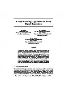
Fig. 1. A point that is an outlier in a 2-dimensional space but not in any of the two corresponding 1dimensional spaces.
The domain of outlier detection (Chandola, Banerjee and Kumar, 2009; Petrovskiy, 2003) deals with the problem of finding such anomalous data, called outliers. Outlier detection can be viewed as a special case of unsupervised binary class separation in the case of ‘rare classes’. The dataset is separated into a large class of ‘normal cases’ and a small class of ‘rare cases’ or ‘outliers’. Outlier detection is particularly problematic as the dimensionality d of the given dataset increases. Problems are often due to sparsity or due to the fact that distancebased approaches fail because the relative distance between any pair of points tends to become relatively the same, see (Beyer, Goldstein, Ramakrishnan and Shaft, 1999). One idea to overcome such problems is to rank outliers in the high-dimensional space according to how consistently they are outliers in low-dimensional subspaces, in which outlierness is easier to assess. To this end, Lazarevic and Kumar developed Feature Bagging (Lazarevic and Kumar, 2005) and He et al. SOE1 (He, Xu and Deng, 2005), both taking an ensemble approach combining the outlier results over subspaces. SOE1 is remarkably simple, summing the local densities of each point for each individual attribute. While SOE1 looks only at 1-dimensional subspaces (i.e., at single attributes), Feature Bagging combines the results of the well-known LOF outlier detection method (Breunig, Kriegel, Ng and Sander, 2000) applied to random subspaces with d/2 or more attributes (out of a total of d attributes). However, both methods have weaknesses. SOE1. Looking only at 1-dimensional subspaces is very efficient but not always effective. It is simple to give examples showing when this may lead to missed information; Figure 1 illustrates such a case. The point in the upper right corner is not a clear outlier with respect to either attribute 1 or attribute 2, but is obviously an outlier in the two-dimensional space. In two dimensions this is obvious, but the likelihood of such a scenario arising and being significant clearly declines as the subspace size increases — due to the phenomenon explored in (Beyer et al., 1999). Feature Bagging. Once the LOF algorithm, applied in the subspaces, becomes less effective (as d/2 rises beyond the dimensionality barrier shown by (Beyer et al., 1999), see Section 2), bagging will become less effective, too. Motivated by that, we propose a method that employs a stable outlier detection algorithm for subspaces of a fixed low dimensionality k, 1 < k 0, P {|f (x) − Ef (x)| ≥ ϵ} ≤ C1 e−C2 ϵ
2
(1)
where C1 , C2 are constants independent of f and d. Thus, the measure is nearly constant and the tails behave, at worst, as a scalar Gaussian random variable with absolutely controlled mean and variance (Donoho, 2000). This principle is not confined to a sphere and has wide applicability. One probabilistic aspect of concentration of measure is that a random variable that depends (smoothly) on the influence of many independent variables, but not especially on any one, is essentially constant at the mean value (Ledoux, 2001). The requirement of smoothness is provided by functions being Lipschitz. 1
A Lipschitz continuous function is such that a line joining any two points on the graph of the function is never steeper than a certain constant, the Lipschitz constant for the function. To prove a finite mean, the constant should be finite.
6
A. Foss et al
Another example is coin tosses. If a coin of unknown bias p is thrown m times, then, from the Chernoff bound, we have ( ∑m ) 2 Xi ∀ϵ > 0, P i − p ≥ ϵ ≤ 2e−2ϵ m (2) m For example, if a balanced coin is thrown once there is complete uncertainty regarding the outcome. If the coin is thrown 1000 times, the number of heads will, in all probability, be rather close to 500. The larger the number of tosses, the more predictable the outcome, which well illustrates the blessing. The other blessings cited by Donoho (Donoho, 2000) are not unrelated to this phenomenon but are not discussed here as they are not directly relevant to this analysis.
3.2. Data Mining and Concentration of Measure CofM is closely related to the law of large numbers and the Central Limit Theorem which are basic to probability theory. Even though we have not seen any explicit reference to CofM in the related data mining literature, results based on probability theory, notably the often cited work of Beyer et al.(Beyer et al., 1999), exploit this phenomenon. Beyer et al. showed that for a large class of problems, distance approximations designed to speed calculations, in particular tree indices, break down above just a few dimensions. Beyer et al. derive their result subject to a condition that the measures examined – interpoint distances – converge on a mean with increasing dimensionality. They showed that this was valid for a wide range of dataset scenarios (Beyer et al., 1999). The phenomenon which makes distance computations decreasingly useful in the high-dimensional space, as shown by (Beyer et al., 1999), is thus a consequence of the convergence on the mean (as in Equations 1 and 2), which is in itself a blessing if we wish to estimate the mean or exploit this convergence. Thus concentration of measure is itself the problem and the blessing. The problem is that individual points or subspaces cease to be ‘special’, i.e. notably different from others, which is the very basis of the notion of outlierness (for example). On the other hand, while this notion is being taken away, determination of the mean c or probability p is being facilitated. One important utility of that with reference to outlier detection is explored in this paper. In particular, we will present an algorithm that will exploit CofM to separate classes by estimating their variances. In the output, the members of each class will tend to collect around specific values related to the class variance. We will demonstrate that the effectiveness of separation improves asymptotically with increasing dimensionality exactly as predicted by the theory.
3.3. Class Separation by Variance Having touched on the key idea, we can proceed to take advantage of both theoretical and empirical work on this measure to prove the following assertion: Assertion 1: In general, an ensemble of subspaces of size m can provide a measure that distinguishes classes {A, B, ..} if each class has (at least) different variances σ, has a Lipschitz distribution and m, the size of the ensemble, is greater than some empirical constant m′ . Let the dataset be D with d independent dimensions and the arity of the subspaces measured be k. We proceed as follows: First we need to show that CofM applies, starting with determining the number of
Class Separation through Variance: A new Application of Outlier Detection
7
x
2
{2,2}
Aj 1
1
Ai
2
Fig. 2. Local density measure example on two attributes.
independent variables in the application. For this, we define an outlier score measure, which can be applied to a subspace, and then estimate the number of independent sets of subspaces in an ensemble. This result is then generalised. This is necessary because if subspaces larger than 1D are combined, it can be objected that these subspaces are not independent as they are made of combinations of the original attributes. Second, if the measure employed converges on its mean, we show that this allows classes with different variance to separate within a ranking of the outlier scores. Consider a two-dimensional subspace {Ai , Aj } (e.g. Figure 2) in which a simple generic approach to outlier determination is followed as in (He et al., 2005) which applies a grid and uses the count in the grid as the (inverse) measure of sparsity for scoring the points. (He et al., 2005) only applied this to the single dimensions but Figure 2 is an example of where there is a clear benefit if a larger subspace grid is used. Let δl (x) be the density measure (cell count) for point x on attribute or attribute set l. In Figure 2 point x has δi (x) = 4, δj (x) = 4, δij (x) = 1. Purely for the sake of this example, let the outlier score over m spaces (each of size 1D, 2D or kD) be ϕ(x) =
m ∑ N δl (x) l
Thus in the 1D analysis, ϕ(x) is accumulated over m (= d) independent variables. In the 2D case, subspaces overlap due to shared attributes but in each space {Ai , Aj } the only dependency of δij (x) on the attributes is an upper (lower) bound provided by exactly inspected such that ( one ) attribute. If all k > 1 size subspaces of d attributes are (d−1 ) m = kd , at most one attribute will provide the upper bound for k−1 subspaces, an(d−2) other for at most k−1 and so forth. This results in a set of at least d−k +1 independent subsets of subspaces of decreasing size where each set has a common dependency, albeit weak. Thus, in the ‘worst case’ scenario, the number of independent measures is still at least d − k + 1. This result applies to any measure that shows a dependence on at most one attribute. If a measure was dependent on a combination of 2 or more attributes, then the number of independent variables would be larger than d as the number of distinguishable subspaces size k > 1 is greater than d. Thus( the ) bound is general to any measure: Any outlier method computed on ensembles of kd subspaces will have at least d − k + 1 independent sets of subspace results. For a fixed k, especially with k ≪ d, this is O(d). So far we have assumed the attributes are independent. This is reasonable because, whatever the dimensionality of a dataset, it can always be transformed into a possibly smaller number of essentially independent dimensions by any of the standard means. Therefore, the concentration of measure phenomenon will apply to the outlier measure ensemble score ϕ if 1) the measures are Lipschitz and 2) the number of attributes
8
A. Foss et al 350
300
250
200 Class 1 Class 2 150
Observed Cluster Boundaries
100
Threshold T 50
0 -x B
0
xB
Fig. 3. Clustering a mixture of two Gaussians.
is sufficiently large for CofM to practically apply. Regarding (1), underlying classes are usually Lipschitz unless strong boundary effects are evident. The measure we are taking here amounts to an estimate of a part of the probability distribution function which will be Lipschitz if the underlying distribution is. Regarding (2), Equation 2 shows an exponential convergence on the mean suggesting convergence even for low dimensionality. The empirical results of Beyer et al. (Beyer et al., 1999) suggest 10-15 dimensions are sufficient. Later we present our results (Section 4.7) showing how this phenomenon rapidly intensifies at similar low dimensionality. Thus we can take m′ ≈ 15. Now we have to show how the classes are separable. Figure 3 shows an example of a difficult case for class separation, separating two concentric classes. There is no spatial differentiation to exploit but the difference in the variance results in one class contributing the majority of the distribution tails. In one dimension, that would only allow us to collect a small number of points from the extreme tails, which likely belong to high variance Class 2. However, as dimensionality increases, CofM means that the points belonging to each class Ci will tend to yield a measure relatively close to some constant ci . If this measure has a dependency on the class variance, then c1 ̸= c2 if the variances differ causing the classes to separate in the measure ranking. Let us consider some common approaches to the problem. Following (He et al., 2005) we can define a measure on each point x based on the local density observed around x. This density will be dependent on the observed distribution which, in Figure 3, is the sum of the probability distribution functions (PDF) of the two classes. However, the position of x relative to the mean is solely due to the PDF of its class Ci . Suppose we take an approach that applies a threshold T and only those points detected in areas with local density below T are inspected (∀x ∈ D | δ(x) < T ). T effectively creates a cluster boundary (e.g. as in Figure 3). We can either define a measure that is based on local density as in the earlier part of this proof or on the distance from the cluster, however defined. This will yield a real value estimate of ‘outlierness’ but is also a direct consequence of the PDF of the underlying class. Alternatively, we can take a binary measure giving equal score to any points found beyond the cluster boundary. However,
Class Separation through Variance: A new Application of Outlier Detection
9
over multiple attributes or subspaces, this measure is again dependent on the PDF of the underlying class since the variance of the class determines the likelihood of the point appearing in the tail. This binary score approach is like the coin flipping case of Equation 2. For a probability distribution function F (N, µ, σ), the outlier measure will converge on the probability pi for attribute i where (assuming no boundary effects) ∫ xB F (N, µ, σ) B pi = 1 − ∫−x ∞ F (N, µ, σ) −∞ If we treat N and µ as constants and set the total cumulative distribution function as C, for example, by normalising the distributions, then 1 f (xB , σ) C making clear the dependence of p on σ. From this we can expect that such an approach to outlier scoring will cause entire classes with different σ to converge their scores around different values. As it has been shown that the tails of the (outlier) measure (for Lipschitz functions) are approximately Gaussian (Equation 1), if we plot the ranked outliers by rank and score for all x ∈ D such that for rank i xi ≥ xi+1 , then each class will produce an ’S’ shaped curve. The outlier score of most points in a class will cluster around some constant giving a close to linear plot with ‘tail’ points having scores increasingly larger (smaller) than this constant. Exactly this can be seen in both synthetic and real datasets in the figures in Section 6.2. Thus, as postulated, classes with different variances will tend to separate in an outlier ranking. Therefore, under the appropriate conditions discussed, the assertion is accepted. pi = 1 −
The intuition behind this in terms of an outlier method can be expressed as follows: If a point is contained in a class of high variance, then this point is likely to be an ‘outlier’ in many low-dimensional subspaces, and vice versa. Let us explain this intuition in more detail, assuming a density-based Outlier method applied in k-dimensional subspaces. First, assume a point x is ranked high in the outlier ranking. Then, for ‘many’ kdimensional subspaces DS of D, where S = {i, j, ...}, |S| = k, x is assigned a high outlier degree in DS by the corresponding Outlier method. This means that, for ‘many’ subspaces DS of D, x is isolated (i.e., an outlier). Suppose two classes {A, B} where the variance of A is less than that of B. Since the class A has low variance, points in A are expected to be not isolated in ‘most’ k-dimensional subspaces. Hence x is more likely to belong to B than to belong to A. Consequently, if a point has a score value above a certain threshold, this point is most likely to belong to B. Second, assume a point x is ranked low in the outlier ranking. Then, for ‘most’ k-dimensional subspaces DS of D, x is not considered an outlier in DS by the corresponding Outlier method. This means that, for ‘most’ subspaces DS of D, x is in a dense region. Since the class B has high variance, points in B are expected to be isolated in ‘many’ subspaces. Hence x is more likely to belong to A than to belong to B. Consequently, if a point has a score value below a certain threshold, this point is more likely to belong to A. In particular, if the difference between the variance of A and the variance of B is sufficiently large, and if d is high enough to provide an adequate number of subspaces,
A. Foss et al
Outlier Score
10
Rank
cv
Example (ii)
Outlier Score
Example (i)
Rank
Fig. 4. In Example (i) two classes with equal variance show no separation in the outlier ranking. In Example (ii), the difference in variance leads to a degree of separation.
we expect thus to separate basically all points in B from all points in A — just because basically all points in B will have higher outlier scores than any point in A. Since this observation is totally independent of the mean µ around which the points in a class are distributed, our algorithm works well even if two classes overlap completely — as long as the two classes differ significantly in variance. Figure 4 illustrates the general phenomenon. In Example (i), there are two equal variance classes and this results in their members being well mixed in the outlier score ranking. However, in Example (ii), the variances of the two classes are different and there is a tendency for the higher variance class cv to populate the higher outlier score rankings. If the classes are heavily overlapping, in any given subspace, only a few members of cv will visually appear as outliers. However, as their underlying variance is higher, accumulating over multiple subspaces, eventually almost all can differentiate themselves from the lower variance class. In fact, for many real-world datasets it is the case that they contain two or more classes that differ significantly in variance. For instance, when considering medical data, it is often the case that the class representing healthy cases has lower variance than the class representing unhealthy cases. To date, outlier detection has been understood as beneficial in separating two such classes in the case of an extreme class imbalance, i.e., if the ‘healthy’ class is predominant in the sense that it contains many more data points than the ‘unhealthy’ class. However, our outlier detection method allows for unsupervised class separation even in the case of perfectly balanced classes, as long as the classes differ in variance. In this section, we have seen that an approach that sums or computes a mean of outlierness for data points over an ensemble of variables, here outlier scores in different subspaces, should cause classes with different variances to separate. In this section, we anticipated that, due to Concentration of Measure, separation should intensify exponentially with increasing dimensionality. In the following sections, an algorithmic approach is proposed which analyses ensembles of subspaces and this effect is extensively investigated. As will be seen, the results are in line with the theoretical expectations.
Class Separation through Variance: A new Application of Outlier Detection
11
4. Methodology: FASTOUT The algorithm FASTOUT employs a novel subspace ensemble outlier detection approach based on a new linear cost nearest neighbour technique. This approach can exploit an arbitrary size of subspace rather than 1D (He et al., 2005), 2D (T*ENT, T*ROF) or αD, where α ≥ d/2 for d dimensions (Lazarevic and Kumar, 2005). We also show that only a sample of all the possible subspaces is sufficient to achieve high effectiveness, making it very efficient. Earlier we discussed various approaches to outlier scoring (See, for example, Section 2, Table 1). In particular, it was shown that a binary scoring based on ‘clustered’/‘notclustered’ in each subspace accumulated over sufficient subspaces (to be defined later) should provide the desired potential for class separation on the basis of differences in class variance. We therefore developed an efficient and effective algorithm for clustering within a given subspace (of any size), using an efficient nearest neighbour scheme. The algorithm is referred to as FASTOUT. We start by providing certain definitions and then introduce our methodology for exploiting these for outlier detection. We then show how outlier detection can be used to sort, unsupervised, binary or even higher multiple underlying classes even when their distributions are fully overlapping.
4.1. Definitions We assume a dataset D ⊂ Rd with d dimensions A = {1, 2, . . . , d}. For every point x ∈ D and every i ∈ {1, . . . , d} we denote by xi the value in the ith attribute of x, i.e., x = (x1 , . . . , xd ). Definition 4.1. k-Subspace S and subspace projection DS . S = {i1 , . . . , ik } ⊆ {1, . . . , d}. DS is the projection of D on S. Definition 4.2. Subspace (Nearest) Neighbours. Let x, x′ ∈ DS . Then x is a nearest neighbour to x′ with respect to S (an S-NN) iff 1) for any categorical attribute Ai ∈ A, xi = x′i , ∀si ∈ S. That is, the Hamming distance between x and x′ is zero for S; or 2) for any numerical attribute Aj ∈ A, |xi − x′i | ≤ ϵ, ∀si ∈ S for some ϵ ≥ 0. Definition 4.3. Subspace Cluster C. Let x, x′ ∈ DS . Then x is said to be reachable from x′ if there are points n0 , . . . , nz in DS such that x is an S-NN of n0 , nm is an S-NN of nm+1 for all m < z, and nz is an S-NN of x′ . A cluster C in DS is a maximal set of points that are pairwise reachable in DS . Let C = {C1 , . . . , Cm } be the set of all clusters in DS Definition 4.4. Outlier. Let x ∈ D. Then x is an outlier in DS iff ∀Ci ∈ C , x ∈ / Ci or x ∈ Ci , |Ci | < ρ, i.e. Ci is small. OS ∈ DS is the set of outliers for subspace S. Definition 4.5. Outlier Score (Binary). Let x ∈∑D and E = {S1 , . . . , S|E| } be the set of all subspaces. The outlier score ϕ(x) = S∈E f (S, x) where
12
A. Foss et al
{ f (S, x) =
1 0
x ∈ OS otherwise
(3)
Definition 4.6. Outlier Ranking. ∀x ∈ D the outlier ranking is the sorted list {1, . . . , |D|} indexed by i of outlier scores such that ϕ(xi ) ≥ ϕ(xi+1 ).
4.2. Finding Nearest Neighbours In order to find the close neighbours of each point we hash the points into bins on each attribute. The number of bins N umBins is O(|D|) and for attribute Ai M ax(Ai ) − M in(Ai ) (4) N umBins where M ax(.) and M in(.) represent the maximum and minimum values of the points on an attribute. As N umBins is dependent on the size of the dataset, we define a parameter Q independent of dataset size, which is defined as BinW idth(Ai ) =
|D| (5) N umBins Q determines the average number of points in a bin and is O(1) as N umBins is chosen to keep Q a fixed constant. Unless the data is already normalised over some range, a pass over the database allows the minimum and maximum values of each attribute to be computed. From this, the bin width on each attribute is computed and another pass over the data allows the points to be assigned a bin number and a count be made for each bin. Then a |D| × d index can be created of the points sorted in each bin. This allows enumeration of the points in a bin without any searching at the cost of one more pass over the data (Algorithm 4.1). To find the neighbours of a point x ∈ D over subspace S ⊆ A, where the attributes are numerical, we look for all points that are within half a bin width (w/2) of x on all members of S. Let x be in bin j. Then we calculate the distance on attribute si ∈ S over all points in bin j and keep those within w/2 of x. If x is in the first half of the bin j then we repeat over bin j − 1, or, if in the second half, over bin j + 1. This is repeated over all attributes in S keeping only those points that are neighbours on all members of S. For categorical attributes, points with the same value are clustered. This process has a complexity of O(|D|d) with an approximately linear dependency on Q. Q=
4.3. Creating Clusters in Subspaces After collecting a vector v of the nearest neighbours of a point p ∈ D, each member can be assigned a cluster number c. Then all the neighbours of each point u ∈ v, that have not been given a cluster number, are collected and also assigned c. This continues through a recursive process until no more points can be assigned. Since a point is only assigned a cluster number once and the number of nearest neighbours to be inspected is, on average, Q for each dimension, the process is O(Q|A||D|) (Algorithm 4.1).
Class Separation through Variance: A new Application of Outlier Detection
13
Algorithm 4.1 RankedOutliers() – Detecting, Scoring and Ranking Outliers Input sample size sample, subspace size k, parameter Q Output set of points S sorted (ranked) by outlier score ∀a ∈ A Compute Bin Widths (Q) ∀x ∈ D ∀a ∈ A Count Numbers in Bins ∀x ∈ D ∀a ∈ A Assign to Bins for i ← 1 to sample do Choose Random set of k attributes s c←0 for all x ∈ D, x.clustered = 0 do c←c+1 x.clustered ← c Collect vector v of all unclustered points that are neighbours of x or neighbours of members of v ∀a ∈ s {Collect recursively until no additions can be made. Neighbour defined in text} if v = ∅ then x.clustered ← 0 else ∀q ∈ v, q.clustered ← c end if end for for all x ∈ D do if x.clustered > 0 then x.clustered ← 0, x.score ← x.score + 1 end if end for ∀x ∈ D, S ← x end for Sort S by score return S
Algorithm 4.2 Theta() – Gets Ranked Outlier List and Computes θ Input sample size sample, subspace size k, points to rank n, parameter Q Output θ and set of points S sorted (ranked) by outlier score S ← RankedOutliers(sample, k, Q) {Algorithm 4.1} θ ← Number of Points with Score Equal To n in S return {θ, S}
4.4. Outlier Detection All points not assigned a cluster number, due to not having any neighbours or being in a very small cluster, are flagged as outliers in the given subspace (Algorithm 4.1). We have consistently used 1% of the dataset as the minimum cluster size as this proved robust (see Section 4.7).
14
A. Foss et al
Algorithm 4.3 OptimisedRanking() – Automates Parameter Setting Input maximum acceptable value of θ target {normally 1} Input sample size sample, points to rank n Output optimised ranked outlier list S k←3 Q←5 maxQ ← n/4 stepQ ← 10 lastθ ← n {θ, S} ← T heta(sample, k, Q) while (θ > target or θ < lastθ or Q < maxQ) do if (θ ≤ target) then return S end if if (θ ≥ lastθ) then {Effectiveness declining so try next k} k ←k+1 Q ← Q − stepQ {Only need to back up 1 step} lastθ ← n else {Try next Q} Q ← Q + stepQ lastθ ← θ end if {θ, S} ← T heta(sample, k, Q) end while return S
4.5. Outlier Ranking Using Subspaces Given a subspace size k = |S|, all possible subspaces or a sample of them are clustered and the number of times each point is an outlier is tallied. This becomes the outlier score for each point. These scores are then sorted and thus the points are ranked for outlier tendency or ‘outlierness’ (Algorithm 4.1).
4.6. Subspace Sampling Enumerating all possible subspaces, rapidly becomes intractable (even with potential parallelisation of the algorithm). Thus, we experimented with a random sample from all the possible subspaces of a particular size k. Obviously using sampling provides a large benefit in efficiency (see Section 6.4).
4.7. Optimising Parameter Setting Class separation depends on the members of different classes occupying different regions in the outlier ranking and knowing the ranks at which the predominance of one class gives way to the next. Later we will address how these ‘cut’ points may be deter-
Class Separation through Variance: A new Application of Outlier Detection
15
mined. At this stage, let knowledge of these points be assumed. If there are 2 classes, let the cut point be at rank r. If the point at r has score ϕr , let θ be the number of points with identical score ϕr . θ is determined in Algorithm 4.2. FASTOUT has a number of parameters. The key sensitive parameters are subspace size k and bin width Q. For FASTOUT, these are set automatically by Algorithm 4.3 based on an objective. This objective is based on the observation that high accuracy coincides with small θ. For example, Tables 7 and 8 show how values of θ ≃ 1 coincide with the highest accuracy. A minor exception is for k = 2 which tends to produce lower accuracies than k ≥ 3, likely due to the smaller sample size. Algorithm 4.3 scans across a range of values of Q for increasing k until θ = 1 or θ values for the current k are higher than for k − 1 indicating the optimum has already been passed. Normally scans start at k = 3, Q = 5. That θ ≃ 1 is optimal is an empirical observation but it is the condition for the best separation of points in the ranking. For larger values of θ, multiple points have the same outlier score and thus cannot be separated. Thus the accuracies quoted are in themselves approximate. So one would naturally prefer a low value of θ. The algorithm converges rapidly, in our experiments, as θ changes sharply with both k and Q as can be seen from Tabless 7 and 8. We also tested the sensitivity to our choice of 1% of the data size for the minimum cluster size (ρ, see Definition 4.4). On synthetic and real-world data this typically worked well. In some cases in the real-world data, 1% of the data was in low single digits and in these cases a slightly larger value (≈ 10) produced better results. In Algorithm 4.3 a stopping condition maxQ is defined but this limit was never reached in our experiments. It simply reflects the fact that if the number of bins becomes very small, outlier detection is moot.
4.8. Semi-Supervised Class Assignment If we have a ranking in which the classes have separated into different regions of the list and we have some labels, it is possible to attempt to classify unlabelled points based on their proximity to labelled data. No training is implied here but having got a final ranking, the class of each point is predicted based on the votes of the nearest labelled points. The class with the most votes is assigned. Ties are broken arbitrarily. We tested a voting scheme with the nearest z labelled points voting for the class of an unlabelled point x. Varying z from 2 to 10 had very little effect on the results on all test datasets except in case of very small classes and larger z. Thus z = 2 was adopted.
4.9. Large Datasets and a Real Valued Measure The binary ‘clusterd/not clustered’ measure for outlier scoring has two key advantages. First, it is easy to motivate on the basis of Equation 2 and Theorem 1. Simply put, if a point is not clustered it is likely in the tail of whatever distribution it might belong to and we do not, therefore, have to determine that membership. If we proposed a realvalued measure based on the distance from its distribution mean (for example) and there were several clusters found, it would be very difficult to justify which cluster to take. Selecting the nearest would obviously be unsafe as normal and many other distributions have infinite tails. Second, the binary approach provides an effective way of automatically setting the key parameters. On the other hand, the binary approach has certain disadvantages. If the dataset is
16
A. Foss et al
very large and thus, for efficiency, the ensemble size m ≪ |D|, θ, the number of coequal points can become large. This has implications for finding class boundaries and the semi-supervised assignment of class labels (Section 4.8) may be influenced by artifacts in the presentation order of the data. One way of handling the later is to randomly sort the data prior to scoring and the semi-supervised approach can be applied to the sorted but unscored data to provide a base line, which amounts to guessing based on the label frequency in the training data. Both these approaches are applied in Section 6.7 for the analysis of intrusion detection. However, while these two strategies can give us confidence in the results, they do not resolve the main issues. It would, therefore, be advantageous to find a real-valued measure that satisfactorily reproduces the characteristics of the binary measure ϕ. The binary measure’s differentiation of points is related to the frequency of points similarly scored on the subspace. That is, if a point is not clustered but most others are, then its score will have more weight on the final result than if many points are not clustered. To capture this, a measure ϕR is defined that is the normalised inverse product of the entropy of the point and the entropy of the subspace. That is, for a point |C | i in cluster Cj where pi = pCj = |D|j 1 2 log( |D| ) ∑ ϕR = |D|pi log(pi ) Ck ∈C pk log(pk )
(6)
Thus ϕR decreases both due to the point being in a larger cluster (less likelihood of being an outlier) and to the higher entropy of the subspace (many outliers). ϕR provides a strongly non-linear bias to exceptional outliers. ϕR ∈ [1, ∞[ but the asymptote occurs when all points are in a single cluster and that is not scored. This modification of FASTOUT is referred to as FASTOUT-R. Since ϕR can not be optimised in the same way as ϕ using θ ≈ 1 as an objective but gives similar results to ϕ with the same parameters on the synthetic data, fixing k and Q can be done by using the binary approach with a small ensemble (for efficiency) and choosing the k and Q that give a θ minimum to use for scoring the data with ϕR . All the results are for the binary approach except in Section 5 and Section 6.7 as the purpose is to demonstrate the phenomenon of class separation in the most straightforward way.
4.10. Categorical Attributes Large datasets typically contain a mixture of categorical and real valued/multinomial data. FASTOUT handles categorical values automatically as indicated in Definition 4.2.
4.11. The γ Heuristic With some categorical attributes and large |D| it could occur that a point exists in very dense bins on all attributes of a subspace. This results in a large cluster being discovered and is an unnecessary cost for outlier detection. Since all attributes are binned, this issue extends to all attribute types. Therefore a heuristic was added to FASTOUT-R that if the least dense bin inhabited by a point is larger than γ|D|, the point is not classed as an outlier but placed in a cluster with all other such points. This heuristic is purely optional and improves efficiency without any significant effect on accuracy. This was only used on the KDD Cup 99 data with γ = 0.01 (Section 6.7).
Class Separation through Variance: A new Application of Outlier Detection
17
Table 2. Class sizes, dataset size and number of attributes.
Ionosphere SPECTF Sonar WDBC Parkinsons Spambase Creditcard Musk Insurance
|D|
d
Target class
Other class
351 267 208 569 195 4601 1000 476 5822
32 44 60 30 22 57 24 166 85
126 212 111 212 148 1813 700 207 348
225 55 97 357 48 2788 300 269 5474
5. Experimental Results The new and comparison algorithms were tested on all UCI Repository (Blake and Merz, 1998) binary problem datasets, with 20 or more attributes, which they would all reasonably be expected to complete. This meant requiring non-categorical data without missing values or a very large number of attributes (≥ 500) since most contender algorithms could not handle all of these. While these limitations could be reduced by modifying certain of the algorithms, they serve as a useful set of conditions to define a group of datasets that is both broad in scope and free of any question of experimenter bias. Out of the 12 datasets that meet these criteria, two were left out each being one of a pair of datasets based on the same data. For example, the SPECTF data with the highest number of attributes was chosen. The ’Hill-Valley’ dataset was omitted since the task should not be amenable to this approach. Whether a sequence has a peak or a trough does not imply any likely difference in variance between the classes. On the other datasets, it is reasonably possible that the two classes may have different variances due to some meaningful tendency in the data. Table 2 gives an overview of these datasets showing that they represent various class balances including a preponderance of the class B expected to be more often contributing outliers. Hardly any would meet the usual ‘rare’ class criterion. For example, the WDBC set consists of 569 samples labelled in two classes, 212 malignant and 357 benign with 30 attributes for each sample. In this dataset as in many medical scenarios, normal biopsies tend to have quite strongly clustered results while abnormal ones exhibit a higher variance. The results on the UCI datasets are summarised in Tables 3 and 4. Our results show that overall FASTOUT and our previously reported algorithms T∗ ROF and T∗ ENT (Foss et al., 2009) were the most effective though Robust Mahalanobis Distance (RMD) (Rousseeuw and Driessen, 1999) and SOE1 (He et al., 2005) performed well. RMD is also hampered by high run time and SOE1 by parameter sensitivity. The most effective approaches also require minimal parameter setting. T∗ ROF is parameter free and FASTOUT automatically adjusts its parameters. These therefore have a clear edge as effective and user friendly approaches. An extensive, but not necessarily exhaustive, literature search for the best results on these datasets using supervised classifiers yielded the following: Ionosphere: Wang (Wang, 2006) using a range of kNN classifiers and 10-fold crossvalidation (MCV) achieved an accuracy of 87.8%. A Support Vector Machine (SVM) ensemble tested with 10-fold MCV achieved 95.20% (Kim and Park, 2004). SPECTF (Cardiac): Previously, the CLIP3 algorithm was used to generate classification rules that were 81.34% accurate (as compared with cardiologists’ diagnoses)
18
A. Foss et al
Table 3. Area under the curve (AUC) and percent accuracy on the target class for various UCI datasets. †Could not compute covariance matrix. Ionosphere AUC
%
SPECTF
Sonar
WDBC
Parkinsons
AUC
%
AUC
%
AUC
%
AUC
%
FASTOUT FASTOUT-R T*ROF T*ENT
0.8400 85.78 0.8297 85.33 0.8915 74.60 0.8429 84.89
0.7816 0.7915 0.8849 0.8959
87.74 87.74 90.57 92.45
0.6449 0.5894 0.9255 0.6235
62.16 60.36 83.51 61.26
0.9578 0.9211 0.9574 0.8474
87.74 82.08 87.74 85.85
0.7514 85.71 0.6835 82.99 0.7405 83.67 0.5319 80.27
SOE1 FBAG LOF ORCA RMD T*LOF
0.7691 0.6048 0.5836 0.4575 0.9479 0.4297
0.7642 0.436 0.4154 0.5569 0.7527 0.3753
84.43 78.30 77.83 80.19 84.36 75.94
0.601 56.76 0.5018 54.05 0.4954 54.96 0.5056 49.48 0.5857 62.73 0.4836 52.25
0.9203 0.5161 0.4699 0.5091 0.9131 0.4834
80.66 39.63 35.85 39.62 77.25 38.21
0.7456 0.4239 0.4386 0.5169 † 0.4249
80.00 69.78 66.22 60.89 87.40 63.56
80.95 72.11 72.79 76.19 72.79
Table 4. Area under the curve (AUC) and percent accuracy on the target class for various UCI datasets. †Could not compute covariance matrix. *Exceeded time limit. Spambase
Credit Card
Musk
Insurance
AUC
%
AUC
%
AUC
%
AUC
FASTOUT FASTOUT-R T*ROF T*ENT
0.7294 0.7255 0.9077 0.7278
59.96 72.74 79.15 78.26
0.4675 0.5274 0.3237 0.7689
69.29 72.00 63.14 89.14
0.6911 0.7736 0.7055 0.3297
72.12 69.57 58.45 28.99
0.5363 0.4763 0.5213 0.5386
8.05 8.33 4.31 10.06
SOE1 FBAG LOF ORCA RMD T*LOF
0.7078 0.4742 0.4668 0.4909 † 0.4825
58.36 37.51 36.62 38.44
0.4422 0.5201 0.494 0.5551 † 0.5168
69.14 68.57 69.14 71.71
0.3359 0.4967 0.4906 0.5084 † 0.4958
29.95 43.48 43.00 46.38
0.5489 0.4999 0.4994 0.5359 † *
10.63 8.33 6.61 8.62
39.33
71.57
42.51
%
(Kurgan, Cios, Tadeusiewicz, Ogiela and Goodenday, 2001). Ali et al. (Ali, Rueda and Herrera, 2006) report that the best Linear Dimensionality (LD) reduction Quadratic classifier had an error of 4.44% while the LD Linear classifier studied had an error rate of 17.64%. Sonar: The Sonar dataset is known to be difficult to separate. Harmeling et al. (Harmeling, Dornhege, Tax, Meinecke and M¨uller, 2006) tested a wide variety of supervised methods including Gaussian mixtures, Support Vector Data Description (SVDD), Parzen, a k-means based approach, and several k-NN methods. Their concept was using various Table 5. Subspace size and Q determined by FASTOUT for the results in Tables 3 and 4.
Ionosphere SPECTF Sonar WDBC Parkinsons Spambase Credit Card Musk Insurance
k
Q
3 4 5 5 5 4 4 7 4
5 25 25 60 45 5 25 75 25
Class Separation through Variance: A new Application of Outlier Detection
19
local density based measures to rank the points for their degree of being typical, as an outlier method does. Results varied from AUC 0.596 (SVDD) to 0.870 (new γ kNN method). WDBC: Jiang and Zhou used a neural network to edit the training data for kNN classifiers (Jiang and Zhou, 2004). With a minimum of 250 points used as training data, 100% separation of the classes was been achieved. With 200 training points they achieved 96% accuracy. Ali et al. (Ali et al., 2006) report that the best Linear Dimensionality (LD) reduction Quadratic classifier had an error of 4.02% while the LD Linear classifier studied had an error rate of 2.99%. Parkinsons: No comparable supervised classification results were located in our literature search. Spambase: Neural Expert networks have been reported with an accuracy of 85% (Petrushin and (Eds), 2007) using 10 fold MCV. Credit Card: This is the Statlog (German Credit Card) dataset. Eggermont et al. used Genetic Programming and compared with C4.5 with Bagging and Boosting and other algorithms. The best result was a 27.1% misclassification rate (Eggermont, Kok and Kosters, 2004). Musk: This is a highly studied dataset. For example, Zafra and Venture report accuracy with SVMs of 87% and 93% with a genetic algorithm (Zafra and Ventura, 2007). This dataset is only nominally two-class as both musks and non-musks are made up of multiple classes and thus is possibly not suitable for the outlier approach. Insurance: This was part of the COIL 2002 competition and proved difficult for all algorithms. Caravan ownership is to be predicted based on other factors in an insurance application. The best results were only a few percentage points better than the best in Table 4 (See e.g. (Zadrozny and Elkan, 2002)). The very best supervised classifiers outperform the outlier methods on most datasets tested but the margins are generally small. Remarkably, one of our unsupervised approaches achieved the best result on two datasets – Sonar (T*ROF) and Credit Card (T*ENT). FASTOUT, FASTOUT-R, T*ENT and T*ROF are remarkably competitive considering that they simply exploit the difference in variance between the classes and operate unsupervised. Obviously, different datasets are suited to different algorithms but overall FASTOUT and T*ROF put in the best performance with respect to effectiveness. FASTOUT-R is significantly more efficient, requiring 25% or less subspace sample size to produce similar results to FASTOUT which is, itself, substantially more efficient than the T* methods that fully enumerate the 2D subspaces.
6. Further Exploring Class Separation with FASTOUT In order to elicit the understanding of the concept of class separation through variance, it is advantageous to investigate synthetic datasets with known characteristics. After that, we look at the scheme that classifies using the outlier ranking and a small proportion of labelled data. These experiments were performed using a 2.6GHz AMD processor and 2G of RAM. All the results in this section are for the binary scored approach (FASTOUT) except in Section 6.7 as the purpose is to demonstrate the phenomenon of class separation in the most straightforward way. In Section 6.7, a large database is studied that requires the greater efficiency of FASTOUT-R.
20
A. Foss et al Weakly Overlapping Dataset DS1w
Fully Overlapping Dataset DS1f 35
30
30
20 Series1 Series2
15 10 5
Attribute 30
Attribute 30
25
25 20
Series1 Series2
15 10 5
0
0 0
5
10
15
20
25
30
0
5
[t]
10
15
20
25
30
35
Attribute 29
Attribute 29
Fig. 5. Example plots of the weakly and fully overlapping datasets DS1w and DS1f on two typical attributes. Table 6. Synthetic datasets with d identical attributes and their classes in the form {N, µ, σ} (size, mean, standard deviation); ri indicates randomly assigned location on each attribute. Designation
d
Classes
DS0w DS1w DS2w DS1f
30 30 30 30
{500, r1 , 2}, {500, r2 , 2} {500, r1 , 2}, {500, r2 , 3} {500, r1 , 2}, {500, r2 , 4} {500, 0, 2}, {500, 0, 3}
6.1. Synthetic Datasets We hypothesised that if a dataset contained two clusters with different variances, then the two groups of points can be separated because the points with the greater variance will be outliers more often. If the variances are the same, then this should fail. This is illustrated in Figure 4. While the outliers are all scored correctly, only in the case where the underlying classes differ in variance do their members’ scores inhabit (largely) different regions of the outlier ranking. We investigated this effect with synthetic datasets with weakly spatially overlapping clusters, labelled ‘w’, and then with fully overlapping clusters, labelled ‘f’. E.g. DS1f means fully overlapping classes with standard deviation differing by 1. Figure 5 illustrates these two cases in a sample 2D space. Table 6 lists the characteristics of the data sets. All the datasets contain classes with Gaussian distributions over all attributes differing only in class size, variance and in some cases class mean µ. Two scoring approaches are taken. First, for binary class data the area under the ROC curve (AUC) is computed. Second, if the class C with the highest variance has size n, then the percentage of members of C in the top n ranked outliers is computed. This is referred to as the ‘accuracy’. If there are several classes, then the percentage of the class found in the expected region of the ranking is quoted as the accuracy. These two measures tend to be closely related so both values are not always given in the results. Table 7 shows the results for the weakly overlapping datasets. This shows very clearly that this approach can separate classes based on a variance difference. Even with classes σ = 2 vs. σ = 3, 100% of the class members appeared in distinct regions of the outlier ranking. On the other hand, where there was no difference in variance (Dataset DS0w), no separation took place. This is as postulated in the theoretical discussion (Section 3). A more challenging case is when the classes are concentric as we might expect the central core of the cluster to contain indistinguishable members of both classes. Table 8 shows that, with the right parameter setting, a 94.0% separation occurs for DS1f. Figure 6 shows that over a range of dimensions from 5 to 60, AUC values quickly rise to better
Class Separation through Variance: A new Application of Outlier Detection
21
Table 7. Effectiveness in separating two clusters in synthetic datasets. Q = 35, Sample = 2000. Accuracy values above and θ values below (see Section 4.7). *All points are equally outliers. k DS0w DS1w DS2w
1
2
3
4
5
49.8% 58.4% 59.4%
50.0% 93.0% 97.8%
48.6% 100% 100%
* * 95.8%
* * *
894 672 760
12 2 4
4 1 1
1000 1000 523
1000 1000 1000
θ, DS0w θ, DS1w θ, DS2w
Table 8. Effectiveness on the fully overlapping dataset DS1f, d = 30 for various Q and sample size 2000. Accuracy values across subspace sizes k above and θ values below. *All points are equally outliers. k Q=35 Q=70 Q=100 θ, Q = 35 θ, Q = 70 θ, Q = 100
1
2
3
4
5
68.4% 58.0% 53.4%
93.2% 88.8% 89.4%
76.4% 92.6% 94.0%
* 85.0% 91.0%
* * 85.0%
709 883 924
3 13 33
75 1 1
1000 14 2
1000 1000 28
than 0.99 (at d ≥ 40). Thus, given sufficient dimensions, the concentric case is only slightly more difficult than the weakly overlapping case.
1 0.95
AUC
0.9 0.85 100 0.8
1000
0.75 0.7 0
10
20
30
40
50
60
70
Dimensionality
Fig. 6. AUC at different dimensionalities for DS1f type datasets at two different sampling sizes.
22
A. Foss et al
Table 9. Synthetic datasets with identical attributes A and their classes in the form {N, µ, σ} (size, mean, standard deviation); ri indicates randomly assigned location on each attribute. ‘U’ in the dataset name indicates containing unbalanced classes. Dataset
d
DS3f DS4f DS4Uf DS4U2f DS4U3f
30, 60, 90 30 30 30 30
Classes {500, 0, 2}, {500, 0, 3}, {500, 0, 4} {500, 0, 1}, {500, 0, 2}, {500, 0, 3}, {500, 0, 4} {500, 0, 1}, {100, 0, 2}, {500, 0, 3}, {100, 0, 4} {30, 0, 1}, {100, 0, 2}, {300, 0, 3}, {500, 0, 4} {15, 0, 1}, {30, 0, 2}, {30, 0, 3}, {500, 0, 4}
Table 10. Separation of 3 fully overlapping clusters of differing variance (DS3f with d = 30) Class (Deviation σ) Ranked Points Top 500 Mid 500 Bottom 500
4
3
2
85.4% 14.6% 0%
14.6% 79.4% 6.0%
0% 6.0% 94.0%
6.2. Multiple Class Separation Having confirmed that both non-concentric and concentric classes can be separated and that separating concentric classes is a more difficult task, we now consider only such classes. So far only balanced classes were analysed. Table 9 shows the characteristics of a number of synthetic datasets with multiple classes and both balanced and unbalanced class sizes. Tables 10, 11 and 12 show the effectiveness of FASTOUT for three class synthetic data DS3f {C1 , C2 , C3 } at three different dimensionalities. There is a clear improvement in separation with increasing dimensionality. Tables 13, 14, 15 and 16 show that this effectiveness of separation extends to 4 classes even if the classes are unbalanced (Datasets DS4f, DS4Uf, DS4U2f and DS4U3f). This data shows that large low variance classes separate well as do high small variance classes relative to them (e.g. Table 16). However, larger higher variance classes can partially overlap with smaller classes of similar variance. For example, σ = 3 and σ = 4 classes separate with markedly lower effectiveness than σ = 2 and σ = 4 classes. It is clear that the greater the difference in variance as well as the larger the dimensionality, the greater the effectiveness of separation. This is well illustrated in Figure 6 and Tables 10 and 11.
Table 11. Separation of 3 fully overlapping clusters of differing variance (DS3f with d = 60) Class (Deviation σ) Ranked Points Top 500 Mid 500 Bottom 500
4
3
2
94.0% 6.0% 0%
6.0% 92.2% 1.8%
0% 1.8% 98.2%
Class Separation through Variance: A new Application of Outlier Detection
23
Table 12. Separation of 3 fully overlapping clusters of differing variance (DS3f with d = 90) Class (Deviation σ) Ranked Points Top 500 Mid 500 Bottom 500
4
3
2
96.8% 3.2% 0%
3.2% 96.6% 0.2%
0% 0.2% 99.8%
Table 13. Separation of 4 fully overlapping clusters of differing variance (DS4f). Class (Deviation σ) Ranked Points Top 500 Next 500 Next 500 Bottom 500
4
3
2
1
77.8% 22.2% 0% 0%
22.2% 70.4% 7.4% 0%
0% 7.4% 92.6% 0%
0% 0% 0% 100.0%
6.3. Class Variance Estimation Consider the 3 class synthetic data presented above (DS3f). This dataset consists of 3 normal distributions {C1 , C2 , C3 } = {{0, 2}, {0, 3}, {0, 4}} where each Gaussian is defined by its mean and standard deviation {µ, σ}. Figure 7 shows 3 fully overlapping Gaussians. The cumulative probability distribution (Φ) for a Gaussian evaluated up to (cluster boundary) XB is Φ(µ, σ, XB ) =
1 √ σ 2π
∫
XB
e
−(u−µ)2 2σ 2
du
(7)
−∞
The binary valued process of outlier detection first clusters and then assigns an outlier score of 1 to points falling outside the cluster. Earlier (Section 3) it was argued that, summing over multiple subspaces, is sufficient to permit an estimation of the probability of a point being an outlier. If this is so, then the cumulated outlier score of a class should approximate the cumulative probability distribution (Equation 7) with respect to the boundary of the cluster ±XB . That is, for the points xj , 1 ≤ j ≤ Ni in Ci = {Ni , µi , σi } 1 ∑ ϕ(xj ) ≃ α Φ(µi , σi , XB ) Ni
(8)
Ci
where α is a constant of proportionality for constant subspace size. If we set the approximate boundary of the clustering of DS3f, say, at XB = 5.1, then Table 14. Separation of 4 fully overlapping unbalanced clusters of differing variance (DS4Uf). Class (Deviation σ) Ranked Points Top 100 Next 500 Next 100 Bottom 500
4
3
2
1
60.0% 40.0% 0% 0%
8.0% 89.8% 2.2% 0%
0% 11.0% 89.0% 0%
0% 0% 0% 100.0%
24
A. Foss et al
Table 15. Separation of 4 fully overlapping unbalanced clusters of differing variance (DS4U2f). Class (Deviation σ) Ranked Points Top 30 Next 100 Next 300 Bottom 500
4
3
2
1
60.0% 40.0% 0% 0%
12.0% 71.0% 17.0% 0%
0% 5.7% 94.0% 0.3%
0.2% 0% 0.2% 99.8%
Table 16. Separation of 3 small and one larger fully overlapping clusters of differing variance (DS4U3f). Class (Deviation σ) Ranked Points Top 15 Next 30 Next 30 Bottom 500
4
3
2
1
93.3% 6.7% 0% 0%
3.3% 96.7% 0% 0%
0% 0% 100% 0%
0% 0% 0% 100%
the relative proportions of Φ(XB ) for the three classes is 3.44%, 29.32%, and 67.24%. If we total the outlier scores for the four classes in the DS3f synthetic dataset, their relative proportions are 2.29%, 30.10% and 67.60%, which is closely similar, given stochastic effects in the randomly generated synthetic dataset and approximations in the numerical integration (Table 17). Dataset DS4f yielded a similar result (Table 17) as also did the unbalanced datasets, for example DS4Uf (Table 18). Thus the binary-valued outlier measure of FASTOUT provides a very good approximation to the probability distribution function for normal distributions. From this we could estimate the σi if we assume normal distributions and can estimate XB relative to µ. Φ for a Gaussian has no closed form solution, so numerical 180 XB 160
140
x10,000
120
100
SD 10 SD 20 SD 30
80
60
40
20
193
181
169
157
145
133
121
97
109
85
73
61
49
37
25
1
13
0
Fig. 7. Three Gaussians with equal mean and differing variance and cluster boundary XB .
Class Separation through Variance: A new Application of Outlier Detection
25
Table 17. Comparison of Σϕ to Φ(XB ) for two synthetic datasets. Σϕ for actual classes. DS3f Class (σ) Σϕ Φ(XB = 5.1)
2
3
4
2.29% 3.44%
30.10% 29.32%
67.60% 67.24%
DS4f Class (σ) Σϕ Φ(XB = 1.6)
1
2
3
4
1.72% 5.73%
24.13% 23.23%
35.36% 32.83%
38.79% 38.21%
Table 18. Comparison of Σϕ to Φ(XB ) for unbalanced class dataset DS4U2f with correction for dataset size N as per Equation 8. Class (σ) N
1
2
3
4
500
300
100
30
(Σϕ)/N 6.56% 27.24% 32.49% 33.71% Φ(XB = 1.2) 9.95% 24.56% 31.03% 34.48%
integration is used to approximate it. The approach we take is an iterative approach where a series of solutions are computed within a reasonable range of the parameters and the best selected and then refined by computing within an increasingly tight region. The ratios of the left hand side of Equation 8 computed for the discovered classes is used as the objective and ratios of the right hand side computed for various values of σ and XB with progressive refinement to give a fit within some ϵ. Thus α drops out. Excellent solutions already exist for separating classes with well separated means. The approach described here is of special utility for the difficult case of heavily overlapping classes and this permits us to assume the means are approximately identical. Therefore, for spherically symmetric distributions, we can assume an approximately spherical form of the clustering which can be captured by its radius XB , rather than some complex shape. This assumption is only relevant if we try to reverse engineer the variances from the outlier scores. It should be noted that the approach of this section does not require a Gaussian or any other specific distribution and thus should apply to any continuous tailed distribution.
6.4. Sampling Full enumeration (F E) of all subspaces is intractable for larger k. Therefore we investigated sampling. If the sample size is S ′ then the number of subspaces summed for the outlier measure S ∗ = min(S ′ , F E). Sampling was tested on DS1f over d = 5 to 60 for S ′ = {100, 1000}. Figure 6 shows the results. In our other experiments a similar pattern emerged with only a small effectiveness gain for larger samples or full enumeration.
6.5. Scaling Synthetic datasets are often used for demonstrating scaling. The advantage is that the structure of the data is known but the disadvantage is that the simple type of datasets often used may not adequately test the algorithms. Purely for the purpose of this scal-
26
A. Foss et al Scaling by Dataset Size 5000 4500 4000
FASTOUT
3500
T*ENT
Secs
3000
T*ROF
T*ENT T*ROF
2500
SOE1 FBAG
2000
ORCA
1500
RMD
1000
LOF
500 0 569
5,690
28450 Points
56,900
FASTOUT SOE1 ORCA
Fig. 8. Scaling by dataset size for comparison outlier algorithms.
ing experiment, the WDBC dataset was used as a seed to create datasets 10×, 50× and 100× the size. This was done by creating multiple points from each point adding a random amount of jitter to each, not exceeding 1%, thus preserving the core characteristics of the dataset. The class labels cannot be applied safely to these larger datasets so no investigation was made into effectiveness. Similarly, to test scaling with respect to the number of attributes, the WDBC data was used as a seed with up to 10% jitter to minimize correlation effects. Figure 8 shows run time over increasing dataset sizes and Figure 9 shows run time over increasing dimensionality. The data can be found in Table 19. RMD, Feature Bagging (FB) and T*LOF could not complete the larger datasets in a reasonable time. This is because RMD is cubic in complexity due to the matrix manipulation and FB has a run-time of about 50 x LOF which is itself ( ) quadratic for higher dimensionality where tree indices are not helpful. T*LOF is kd × LOF and run times are not shown in the Figures but appear in Table 19. While T*ENT and T*ROF scale reasonably, FASTOUT, SOE1 and ORCA are highly efficient. The efficiency of FASTOUT reflects both the efficiency of the algorithm and the use of sampling. FASTOUT-R results are not given because the core algorithm has the same efficiency as FASTOUT but is usually run at a smaller sample size so the net efficiency is even greater by the relative sample size. The γ efficiency heuristic was not employed in any of these experiments. If applied, it further enhances the efficiency of the FASTOUT and FASTOUT-R algorithms.
6.6. Automatic Class Separation In Section 3.3 it was theoretically anticipated that the shape of the outlier ranking graph would exhibit an ‘S’ shape for each class of different variance as long as the class had a smooth probability distribution function. This is clearly visible in Figure 10 especially for the highest variance class in the d = 30 case and all the classes where d = 60. The higher the class variance, the larger the class mean outlier score and the other scores are concentrated around this value (region R2, Figure 10 lower left) with a spreading out at the extreme of each tail (regions R1 and R3). As the relative difference between the
Class Separation through Variance: A new Application of Outlier Detection
27
Scaling by Attributes 3000 2500
FASTOUT T*ENT
Secs
2000
T*ROF SOE1
1500 FBAG
T*ENT T*ROF
ORCA
1000
RMD LOF
500
FBAG FASTOUT LOF ORCA SOE1
0 30
60
90
120
Attributes
Fig. 9. Scaling by dimensionality for comparison outlier algorithms.
Table 19. Run time: scaling by dataset size for various algorithms (30 attributes) and scaling by number of attributes (569 data points). †Could not complete. Algorithm
FASTOUT T*ENT T*ROF SOE1 FBAG LOF ORCA RMD T*LOF
Dataset Size
# Attributes
569
5,690
28450
56,900
30
60
90
120
0.7 43.4 43.6
7.2 317.4 321.0
43.5 821.0 828.4
96.7 1782.2 1798.3
1.0 43.4 43.6
1.9 174.8 178.3
2.0 405.0 411.5
2.1 704.5 717.0
0.0 20.4 0.5 0.6 188.5 77.7
0.1 1620.5 44.0 0.8 2225.1 5907.9
0.7 † 1309.7 1.0 † †
1.5 † 4331.9 1.2 † †
0.0 20.4 0.5 0.6 188.5 77.7
0.0 30.2 0.8 0.8 729.9 393.7
0.0 42.9 1.2 1.2 1619.1 1178.4
0.1 53.8 1.5 1.2 2635.2 1990.8
variances declines, the overlap between the class outlier score tails increases. While it is clear, in the 30D case, that the SD 2 and SD 4 class members separate well (in fact with 99.4% effectiveness) the SD 3 class overlaps sufficiently so that the upper graph which shows the full rank/score graph does not exhibit any clear ‘join’ between the classes. In the 60D case (Figure 10), the SD 2 and SD 3 classes separate enough that there is an obvious inflexion in the full rank/score graph between them. A smaller, but still clearly visible, inflexion is seen between SD 3 and SD 4. In these cases we can locate these ‘joins’ algorithmically. As the graph is not strictly linear but shows some tendency to a steeper slope in the regions where classes overlap, some simple heuristics can be devised for detecting such locations in addition to either visual inspection or some semisupervised approach.
28
A. Foss et al 30D
60D
1600
3500
1400
3000 2500
1000 800
SD 2
600
SD 3
400
SD 4
Outlier Score
Outlier Score
1200
2000
1st Diff SD 2
1500
SD 3 1000 SD 4 500
200 0
0 0
200
400
600
800
1000
1200
1400
0
1600
500
Point Rank
1000
30D
60D 3500
1600 1400
3000
R1
1200
2500
1000
R2
800
SD 2 SD 3
600
R3
400
SD 4
Outlier Score
Outlier Score
1500
Point Rank
2000 SD 2
1500
SD 3 1000
SD 4
500 200 0
0 0
100
200
300
Point Rank within Class
400
500
0
100
200
300
400
500
Point Rank within Class
Fig. 10. Three class synthetic data (DS3f) with d = 30 and 60 showing improved separation for higher dimensionality. Complete outlier ranking graph at top, ranking within classes at bottom.
Let G be the {ϕ, rank} graph as in Figure 10. The separation or ‘join’ points we wish to identify are associated with inflection points in G. Finding the inflection points is simple in principle as the sign of the second differential of the series changes at these points. The difficulty lies in the small stochastic variations. Dataset DS3f was generated randomly and any realistic dataset will have some stochastic variations. Thus a moving average (N/50 points) was employed to smooth the series and the first differential of that taken. A histogram of the first differential was generated and a low pass filter applied at the most frequent value f . This yields zero values for the most linear regions of G. From the first differential, the peaks of all the regions of non-zero values are taken. As the moving average introduces a ‘delay’ in the peak, the index of the peak is reduced by n/100, i.e. half the window. End-effects will usually occur and are not shown. The result on DS3f, amplified ten times for presentation purposes is seen in Figure 10. In the 30D data, no inflexion is detected but in the 60D data the inflections around 500 and 1000 are well marked (Figure 10, top right). As each class contains 500 points this is essentially correct. Obviously the difference between the σ = 2 and σ = 3 classes will be more pronounced than that between the σ = 3 and σ = 4 classes. Looking for the leading peaks in the smoothed totals of the first differential was more useful than looking for a change of sign in the second differential as this occurs at every peak, whatever size, and is thus more prone to stochastic effects. This approach can be used when a suitable shape is seen in output graph G. Generally, the real world data with which we experimented did not permit sufficient separation to be suited to this. Therefore, in the next section, we propose a semi-supervised approach to extracting the classes from the output.
Class Separation through Variance: A new Application of Outlier Detection
29
6.7. Semi-Supervised Class Assignment In this section, the real-valued measure version of FASTOUT is used, FASTOUT-R, as well as the binary version. FASTOUT-R was developed to deal with very large datasets as discussed in Section 4.9. In order to test the concept of classifying points based on labelled neighbours in the ranked list, the KDD Cup 99 data was used (ACM, 1999). This dataset is for detecting computer intrusion. Attacks on computers can be analysed in different ways. For example (Jiang and Zhu, 2009) assess the behaviour of the attacker. In our approach, we investigate if the variables associated with different types of attack can be distinguished by their inherent variance. Each tuple in the dataset has 41 attributes, 3 being categorical. The winner’s result is reported for the test dataset with 311,029 tuples which has 36 classes. Competitors had access to a large amount of training data though the training data has a different probability distribution from the test data. As FASTOUT/FASTOUT-R does not train, we used only the test data (for which labels are available) and randomly selected 1/3 of this data as available labels, excluding the point to be classified, for the voting scheme after all points were ranked (Prior to this voting, the labels were not seen by the algorithm). From these, only the votes of the 2 nearest labelled items are actually being used. A baseline was computed by applying the scoring scheme on the randomised data vector prior to outlier scoring by FASTOUT/FASTOUTR. This quantifies how well one could do by ‘guessing’ on the basis of the relative label frequencies in the ‘training’ data. The choice of 1/3 is conservative but using even lower ratios only resulted in slightly lower effectiveness. The results for various ratios for the best score reported in Table 22 were {100% : 0.1128, 50% : 0.1195, 33.33% : 0.1232, 25% : 0.1259, 20% : 0.1255}. The classes were combined as indicated by (ACM, 1999) to yield 5 classes (one normal and the others are different types of attack). Cost per item was then computed according to the cost matrix provided by (ACM, 1999), which is shown in Table 21. ACM used this cost to determine the winner. This allows comparison with the quoted Cup results (ACM, 1999) with the provision just mentioned regarding the source of labels for the two methods. It was not expected that the FASTOUT-R approach, which simply exploits differences in variance between the distributions of different classes, would give similar effectiveness to supervised classification. However, the results are strongly suggestive of its practical utility for such applications (Table 20 and 22). The results for both the binary (FASTOUT) and the real-valued measure approach (FASTOUT-R) are given in Table 22. The Cup winner data is taken from (ACM, 1999). The binary scheme achieved a cost between the high accuracy of the real-valued score (FASTOUT-R) and the base line. This was a consequence of the very large number of coequal points due to the small ensemble size relative to |D|. Increasing the sample size for FASTOUT (Binary) by 10× lowered the per item cost by 9%. FASTOUT-R typically runs at smaller sample sizes than the binary-valued measure. Using a sample size of 50 (25% of the lower binary sample) already produces a cost 66.5% of the Cup winner’s cost. Increasing the sample size by 4× improved this to 52.9%. These results were obtained without any training. FASTOUT also did better than subsequent attempts at this problem (e.g. (Li and Ye, 2005), cost 0.2445).
30
A. Foss et al
Table 20. Confusion matrices for FASTOUT and the KDD Cup 99 winner. FASTOUT ( ϕR ) Actual
Predicted
Class
normal
1
2
3
4
% correct
normal 1
57673
589
1782
25
524
95.2%
1402
2294
409
2
59
2
55.1%
5535
778
223123
3
414
97.1%
3
156
12
19
35
6
15.4%
4
2087
268
5736
11
8087
50.0%
% correct
86.3%
58.2%
96.6%
46.1%
89.0%
KDD Cup 99 Winner Actual
Predicted
Class
normal
1
2
3
4
% correct
normal
60262
243
78
4
6
99.5%
1
511
3471
184
0
0
83.3%
2
5299
1328
223226
0
0
97.1%
3
168
20
0
30
10
13.2% 8.4%
4
14527
294
0
8
1360
% correct
74.6%
64.8%
99.9%
71.4%
98.8%
Table 21. Cost matrix provided by KDD Cup 1999 organisers. Actual
Predicted
Class
normal
1
2
3
4
normal
0
1
2
2
2
1
1
0
2
2
2
2
2
1
0
2
2
3
3
2
2
0
2
4
4
2
2
2
0
7. Conclusion This paper introduces a new algorithm FASTOUT to efficiently detect outliers in high dimensional spaces with a subspace ensemble approach. It can handle an arbitrary size of subspace. This paper also develops and investigates the novel concept of separating classes based on variance rather than spatial location based on outlier scores. This distinguishes Table 22. Total cost per transaction for the KDD Cup 99 dataset. Cost is per tuple. Baseline Ensemble size Cost/item
FASTOUT
FASTOUT
FASTOUT-R
FASTOUT-R
Winner
n/a
200
2000
50
200
n/a
0.8854
0.5858
0.5349
0.1551
0.1232
0.2331
Class Separation through Variance: A new Application of Outlier Detection
31
it from statistical and other approaches, which use variance to validate separation generated by exploiting spatial differences. For the first time, we have shown that this can be done successfully even in multiple-class problems (beyond binary) regardless of differences in class size showing that outlier detection has application beyond the traditional problem of finding small numbers of extreme data or rare classes. The novel algorithm FASTOUT sets its parameters automatically and is highly efficient. At the same time, it outperforms the state-of-the-art in outlier detection. Not only does it accurately rank data points for outlierness, but in many cases the ranking graph can be automatically split into sections containing predominantly single classes, hence the class separation – something not previously investigated. We have also demonstrated how FASTOUT can be modified to handle large and challenging problems, even outperforming supervised classifiers without the benefit of training data. This suggests a wide range of applications in traditional areas of outlier detection like computer intrusion and fraud detection as well as other classification problems. It appears that the algorithm can be adapted for real-time use in data streams and this is an interesting area for future work.
References ACM, “ACM KDD Cup ’99 Results,” http://www.sigkdd.org/kddcup/ 1999. Aggarwal, C.C. and P.S. Yu, “Outlier detection for high dimensional data,” in “Proc. ACM SIGMOD Intl. Conf. on Management of Data” 2001, pp. 37–46. and , “An efficient and effective algorithm for high-dimensional outlier detection,” VLDB Journal, 2005, 14 (2), 211–221. Ali, Mohammed Liakat, Luis Rueda, and Myriam Herrera, “On the Performance of Chernoff-Distance-Based Linear Dimensionality Reduction Techniques,” Advances in Artificial Intelligence, 2006, 4013, 467–478. Bay, S.D. and M. Schwabacher, “Mining Distance-Based Outliers in Near Linear Time Randomization and a Simple Pruning Rule,” in “Proc. SIGKDD” 2003. Bellman, Richard, Adaptive Control Processes: A Guided Tour, Princeton University Press, 1961. Beyer, K., J. Goldstein, R. Ramakrishnan, and U. Shaft, “When is “Nearest Neighbor” Meaningful,” in “Int. Conf. on Database Theory” 1999, pp. 217–235. Blake, C.L. and C.J. Merz, “UCI Repository of machine learning databases,” http://archive.ics.uci.edu/ml/ 1998. Breunig, M.M., H.-P. Kriegel, R.T. Ng, and J. Sander, “LOF: Identifying Density-Based Local Outliers,” in “Proc. SIGMOD Conf.” 2000, pp. 93–104. Chandola, V., A. Banerjee, and V. Kumar, “Anomaly Detection: A Survey,” ACM Computing Surveys, 2009, 41 (3). Donoho, David, “High-dimensional data analysis: The curses and blessings of dimensionality,” in “Proc. of the American Mathematical Society Conference on Mathematical Challenges of the 21st Century” 2000. Dubhashi, D. P. and A. Panconesi, Concentration of Measure for the Analysis of Randomised Algorithms, Cambridge University Press, 2009. Eggermont, Jeroen, Joost N. Kok, and Walter A. Kosters, “Genetic Programming for Data Classification: Partitioning the Search Space,” in “Proc. of the 2004 Symposium on applied computing (ACM SAC04” ACM 2004, pp. 1001–1005. Fan, Hongqin, Osmar R. Zaiane, Andrew Foss, and Junfeng Wu, “Resolution-based outlier factor: detecting the top-n most outlying data points in engineering data,” Knowledge and Information Systems, 2009, 19 (1), 31–51. Foss, Andrew and Osmar R. Za¨ıane, “A Parameterless Method for Efficiently Discovering Clusters of Arbitrary Shape in Large Datasets,” in “Proc. of the IEEE International Conference on Data Mining (ICDM’02)” 2002, pp. 179–186. , , and Sandra Zilles, “Unsupervised Class Separation of Multivariate Data through Cumulative Variance-based Ranking,” in “Proc. of the IEEE International Conference on Data Mining (ICDM’09)” 2009, pp. 139–148. Harmeling, S., G. Dornhege, D. Tax, F Meinecke, and K-R M¨uller, “From outliers to prototypes: Ordering data,” Neurocomputing, 2006, 69, 1608–1618. He, Zengyou, Xiaofei Xu, and Shengchun Deng, “A Unified Subspace Outlier Ensemble Framework for
32
A. Foss et al
Outlier Detection in High Dimensional Spaces,” in “Proc. of the 6th International Conference, WAIM 2005” 2005, pp. 632–637. Hido, Shohei, Yuta Tsuboi, Hisashi Kashima, Masashi Sugiyama, and Takafumi Kanamori, “Statistical outlier detection using direct density ratio estimation,” Knowledge and Information Systems, 2009, Online First. Jiang, Xuxian and Xingquan Zhu, “vEye: behavioral footprinting for self-propagating worm detection and profiling,” Knowledge and Information Systems, 2009, 18 (2), 231–262. Jiang, Y. and Z.-H. Zhou, “Editing training data for kNN classifiers with neural network ensemble,” Lecture Notes in Computer Science 3173, 2004. Kim, Hyunsoo and Se Hyun Park, “Data Reduction in Support Vector Machines by a Kernelized Ionic Interaction Model,” in “Proc. of SDM. 2004” 2004. Knorr, E.M. and R.T. Ng, “Finding Intensional Knowledge of Distance-Based Outliers,” in “Proc. VLDB Conf.” 1999, pp. 211–222. Kurgan, Lukasz A., Krzysztof J. Cios, Ryszard Tadeusiewicz, Marek R. Ogiela, and Lucy S. Goodenday, “Knowledge discovery approach to automated cardiac SPECT diagnosis,” Artificial Intelligence in Medicine, 2001, 23, 149. Lazarevic, A. and V. Kumar, “Feature bagging for outlier detection,” in “Proc. ACM SIGKDD” 2005, pp. 157–166. Ledoux, Michael, The Concentration of Measure Phenomenon, Vol. 89 of Mathematical Surveys and Monographs, AMS, 2001. Li, Xiangyang and Nong Ye, “A supervised clustering algorithm for computer intrusion detection,” Knowledge and Information Systems, 2005, 8 (4), 498–509. Milman, Vitaly, “The Heritage of P. Levy in Geometrical Functional-Analysis,” Asterisque, 1988, 157, 273– 301. Petrovskiy, M.I., “Outlier Detection Algorithms in Data Mining Systems,” Program. Comput. Softw., 2003, 29 (4), 228–237. Petrushin, Valerii Aleksandrovich and Latifur Khan (Eds), Multimedia data mining and knowledge discovery, Springer, 2007. Rousseeuw, P.J. and K. Van Driessen, “A fast algorithm for the minimum covariance determinant estimator,” Technometrics, 1999, 41 (3), 212–223. Wang, Hui, “Nearest neighbors by neighborhood counting,” Pattern Analysis and Machine Intelligence, IEEE Transactions on, 2006, 28 (6), 942 – 953. Zadrozny, Bianca and Charles Elkan, “Transforming Classifier Scores into Accurate Multiclass Probability Estimates,” in “Proc. of KDD ’02” 2002. Zafra, Amelia and Sebasti´an Ventura, “Multi-objective Genetic Programming for Multiple Instance Learning,” in “Lecture Notes in Computer Science, Machine Learning: ECML ’07” 2007. Zhang, J. and H Wang, “Detecting outlying subspaces for high-dimensional data: the new task, algorithms, and performance,” Knowl. Inf. Syst., 2006, 10 (3), 333–355. Zhou, Zhi-Hua and Ming Li, “Semi-supervised learning by disagreement,” Knowledge and Information Systems, 2009, Online First.