Classical and Bayesian Approach in Estimation of Scale Parameter of ...

Hindawi Publishing Corporation Journal of Probability and Statistics Volume 2016, Article ID 7581918, 8 pages http://dx.doi.org/10.1155/2016/7581918

Research Article Classical and Bayesian Approach in Estimation of Scale Parameter of Nakagami Distribution Kaisar Ahmad,1 S. P. Ahmad,1 and A. Ahmed2 1

Department of Statistics, University of Kashmir, Srinagar, Jammu and Kashmir 190006, India Department of Statistics and O.R., Aligarh Muslim University, Aligarh, India

2

Correspondence should be addressed to Kaisar Ahmad; [email protected] Received 19 October 2015; Accepted 17 December 2015 Academic Editor: Ram´on M. Rodr´ıguez-Dagnino Copyright © 2016 Kaisar Ahmad et al. This is an open access article distributed under the Creative Commons Attribution License, which permits unrestricted use, distribution, and reproduction in any medium, provided the original work is properly cited. Nakagami distribution is considered. The classical maximum likelihood estimator has been obtained. Bayesian method of estimation is employed in order to estimate the scale parameter of Nakagami distribution by using Jeffreys’, Extension of Jeffreys’, and Quasi priors under three different loss functions. Also the simulation study is conducted in R software.

1. Introduction Nakagami distribution can be considered as a flexible lifetime distribution. It has been used to model attenuation of wireless signals traversing multiple paths (for details see Hoffman [1]), fading of radio signals, data regarding communicational engineering, and so forth. The distribution may also be employed to model failure times of a variety of products (and electrical components) such as ball bearing, vacuum tubes, and electrical insulation. It is also widely considered in biomedical fields, such as to model the time to the occurrence of tumors and appearance of lung cancer. It has the applications in medical imaging studies to model the ultrasounds especially in Echo (heart efficiency test). Shanker et al. [2] and Tsui et al. [3] use the Nakagami distribution to model ultrasound data in medical imaging studies. This distribution is extensively used in reliability theory and reliability engineering and to model the constant hazard rate portion because of its memory less property. Yang and Lin [4] investigated and derived the statistical model of spatial-chromatic distribution of images. Through extensive evaluation of large image databases, they discovered that a two-parameter Nakagami distribution well suits the purpose. Kim and Latchman [5] used the Nakagami distribution in their analysis of multimedia.

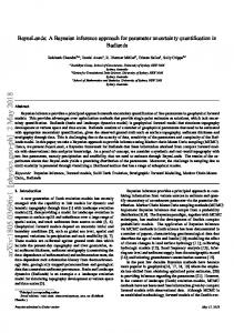
The probability density function (pdf) of the Nakagami distribution is given as mentioned in Figure 1: 𝑓 (𝑦; 𝜃, 𝑘) =

−𝑘𝑦2 2𝑘𝑘 𝑦2𝑘−1 exp ( ) 𝑘 𝜃 Γ (𝑘) 𝜃

(1)

for 𝑦 > 0, 𝑘, 𝜃 > 0, where 𝜃 and 𝑘 are the scale and the shape parameters, respectively.

2. Materials and Methods There are two main philosophical approaches to statistics. The first is called the classical approach which was founded by Professor R. A. Fisher in a series of fundamental papers round about 1930. In classical approach we use the same method as obtained by Ahmad et al. [6]. The alternative approach is the Bayesian approach which was first discovered by Reverend Thomas Bayes. In this approach, parameters are treated as random variables and data is treated as fixed. Recently Bayesian estimation approach has received great attention by most researchers among them are Al-Aboud [7] who studied Bayesian estimation for the extreme value distribution using progressive censored data and asymmetric loss. Ahmed et al. [8] considered

2

Journal of Probability and Statistics which is a symmetric loss function; 𝜃 and 𝜃̂ represent the true and estimated values of the parameter. (ii) The Al-Bayyati new loss function is of the form

f(y)

1.2

1.0 0.8 0.6 0.4 0.2 0.0

̂ 𝜃) = 𝜃𝑐1 (𝜃̂ − 𝜃)2 ; 𝑐 𝜀𝑅, 𝐿 nl (𝜃, 1 0.0

0.5

1.0

1.5

2.0

2.5

which is an asymmetric loss function; 𝜃 and 𝜃̂ represent the true and estimated values of the parameter. (iii) The entropy loss function is given by

3.0

y k = 1.0, 𝜃 = 1.0 k = 1.0, 𝜃 = 1.5 k = 1.5, 𝜃 = 1.0

(7)

k = 1.5, 𝜃 = 1.5 k = 2.0, 𝜃 = 1.0 k = 2.0, 𝜃 = 1.5

̂ ̂ ̂ 𝜃) = ( 𝜃 − log ( 𝜃 ) − 1) ; 𝜃 > 0, 𝐿 ef (𝜃, 𝜃 𝜃

(8)

Figure 1: The pdf ’s of Nakagami distribution under various values of 𝑘 and theta.

where 𝜃 and 𝜃̂ represent the true and estimated values of the parameter.

Bayesian Survival Estimator for Weibull distribution with censored data. An important prerequisite in this approach is the appropriate choice of prior(s) for the parameters. Very often, priors are chosen according to one’s subjective knowledge and beliefs. The other integral part of Bayesian inference is the choice of loss function. A number of symmetric and asymmetric loss functions have been shown to be functional; see Pandey et al. [9], Al-Athari [10], S. P. Ahmad and K. Ahmad [11], Ahmad et al. [12, 13], and so forth.

3. Bayesian Method of Estimation

Theorem 1. Let (𝑦1 , 𝑦2 , . . . , 𝑦𝑛 ) be a random sample of size n having pdf (1); then the maximum likelihood estimator of scale parameter 𝜃, when the shape parameter 𝑘 is known, is given by ∑𝑛 𝑦 2 𝜃̂ = 𝑖=1 𝑖 . 𝑛

(2)

In this section Bayesian estimation of the scale parameter of Nakagami distribution is obtained by using various priors under different symmetric and asymmetric loss functions. 3.1. Posterior Density under Jeffreys’ Prior. Let (𝑦1 , 𝑦2 , . . . , 𝑦𝑛 ) be a random sample of size 𝑛 having the probability density function (1) and the likelihood function (2). Jeffreys’ prior for 𝜃 is given by 𝑔 (𝜃) =

𝐿 (𝑦; 𝜃, 𝑘) =

𝑛

(Γ𝑘)𝑛 𝜃𝑛𝑘

𝑛

∏ 𝑦𝑖

2𝑘−1

𝑖=1

−𝑘 𝑛 exp ( ∑ 𝑦𝑖 2 ) . 𝜃 𝑖=1

𝜋1 (𝜃 | 𝑦) ∝ 𝐿 (𝑦 | 𝜃) 𝑔 (𝜃) .

(3)

𝑖=1

𝑘 𝑛 2 ∑𝑦 . 𝜃 𝑖=1 𝑖

(4)

Differentiating (4) with respect to 𝜃 and equating to zero, we get 𝜃̂ =

∑𝑛𝑖=1

𝑦𝑖

2

𝑛

.

̂ 𝜃) = ( 𝐿 qd (𝜃,

𝜃

(2𝑘𝑘 )

𝑛

𝑛

Γ (𝑘)𝑛 𝜃𝑛𝑘+1

𝜋1 (𝜃 | 𝑦) = 𝜌

∏ 𝑦𝑖 2𝑘−1 exp ( 𝑖=1

1 𝜃𝑛𝑘+1

exp (

−𝑘 𝑛 2 ∑𝑦 ), 𝜃 𝑖=1 𝑖

(11)

−𝑘 𝑛 2 ∑𝑦 ), 𝜃 𝑖=1 𝑖

where 𝜌 is independent of 𝜃 and 𝜌=

(5)

(𝑘 ∑𝑛𝑖=1 𝑦𝑖 2 )

𝑛𝑘

Γ𝑛𝑘

.

(12)

Using the value of 𝜌 in (11),

2.1. Loss Functions Used in This Paper. (i) The quadratic loss function which is given by (𝜃̂ − 𝜃)

𝜋1 (𝜃 | 𝑦) ∝

log 𝐿 (𝑦; 𝜃, 𝑘) = 𝑛 log (2𝑘𝑘 ) − 𝑛 log Γ𝑘 − 𝑛𝑘 log 𝜃 𝑛

(10)

Using (2) and (9) in (10),

The log likelihood function is given by

+ (2𝑘 − 1) ∑ log 𝑦𝑖 −

(9)

By using the Bayes theorem, we have

Proof. The likelihood function of the pdf (1) is given by (2𝑘𝑘 )

1 ; 𝜃 > 0. 𝜃

𝜋1 (𝜃 | 𝑦) 𝑛𝑘

2

) ;

𝜃 > 0,

(6)

=(

(𝑘 ∑𝑛𝑖=1 𝑦𝑖 2 ) Γ𝑛𝑘

1 𝜃𝑛𝑘+1

exp (

−𝑘 𝑛 2 ∑ 𝑦 )) . 𝜃 𝑖=1 𝑖

(13)

Journal of Probability and Statistics

3

3.2. Posterior Density under Extension of Jeffreys’ Prior. Let (𝑦1 , 𝑦2 , . . . , 𝑦𝑛 ) be a random sample of size 𝑛 having the probability density function (1) and the likelihood function (2). The extension of Jeffreys’ for 𝜃 is given by 1 ; 𝜃 > 0. 𝜃2𝑐

𝑔1 (𝜃) =

(14)

where 𝜌 is independent of 𝜃 and 𝑛𝑘+𝑑−1

(𝑘 ∑𝑛𝑖=1 𝑦𝑖 2 )

𝜌=

.

Γ (𝑛𝑘 + 𝑑 − 1)

(23)

Using the value of 𝜌 in (22), 𝜋3 (𝜃 | 𝑦)

By using the Bayes theorem, we have

𝑛𝑘+𝑑−1

𝜋2 (𝜃 | 𝑦) ∝ 𝐿 (𝑦 | 𝜃) 𝑔1 (𝜃) .

(15)

=(

(𝑘 ∑𝑛𝑖=1 𝑦𝑖 2 )

1 𝜃𝑛𝑘+𝑑

Γ (𝑛𝑘 + 𝑑 − 1)

exp (

−𝑘 𝑛 2 ∑ 𝑦 )) . 𝜃 𝑖=1 𝑖

(24)

Using (2) and (14) in (15),

4. Bayesian Estimation by Using Jeffreys’ Prior under Different Loss Functions

𝜋2 (𝜃 | 𝑦) 𝑛

∝

(2𝑘𝑘 )

𝑛

∏ 𝑦𝑖 2𝑘−1 exp (

Γ (𝑘)𝑛 𝜃𝑛𝑘+2𝑐

𝑖=1

−𝑘 𝑛 2 ∑𝑦 ). 𝜃 𝑖=1 𝑖

(16)

̂ 𝜃), the Bayes Theorem 2. Assuming the loss function 𝐿 𝑞𝑑 (𝜃, estimate of the scale parameter 𝜃, if the shape parameter 𝑘 is known, is of the form

Thus 𝜋2 (𝜃 | 𝑦) = 𝜌

1 𝜃𝑛𝑘+2𝑐

−𝑘 𝑛 exp ( ∑ 𝑦𝑖 2 ) , 𝜃 𝑖=1

(𝑘 ∑𝑛𝑖=1 𝑦𝑖 ) . Γ (𝑛𝑘 + 2𝑐 − 1)

(18)

𝜋2 (𝜃 | 𝑦) = (

𝑛𝑘+2𝑐−1

Γ (𝑛𝑘 + 2𝑐 − 1)

∞

̂ =∫ ( 𝑅 (𝜃)

(𝜃̂ − 𝜃)

∞

̂ =∫ ( 𝑅 (𝜃)

(𝜃̂ − 𝜃) 𝜃

0

−𝑘 ∑ 𝑦 2 )) . 𝜃 𝑖=1 𝑖

⋅

3.3. Posterior Density under Quasi Prior. Let (𝑦1 , 𝑦2 , . . . , 𝑦𝑛 ) be a random sample of size 𝑛 having the probability density function (1) and the likelihood function (2). Quasi prior for 𝜃 is given by 1 𝑔2 (𝜃) = 𝑑 ; 𝜃 > 0, 𝑑 > 0. 𝜃

(20)

(𝑘 ∑𝑛𝑖=1

𝜋3 (𝜃 | 𝑦) ∝

Γ (𝑘)𝑛 𝜃𝑛𝑘+𝑑

𝜋3 (𝜃 | 𝑦) = 𝜌

1 𝜃𝑛𝑘+𝑑

𝑛

∏ 𝑦𝑖 𝑖=1

2𝑘−1

−𝑘 𝑛 exp ( ∑ 𝑦𝑖 2 ) 𝜃 𝑖=1

−𝑘 𝑛 exp ( ∑ 𝑦𝑖 2 ) , 𝜃 𝑖=1

) 𝜋1 (𝜃 | 𝑦) 𝑑𝜃.

(26)

2

) (27)

2 𝑛𝑘

𝑦𝑖 )

1

exp (

𝜃𝑛𝑘+1

Γ𝑛𝑘

𝑛

−𝑘 ∑ 𝑦 2 ) 𝑑𝜃. 𝜃 𝑖=1 𝑖

On solving (27), we get ̂ = 𝑅 (𝜃)

𝜃̂2 Γ (𝑛𝑘 + 2) Γ𝑛𝑘 (𝑘 ∑𝑛𝑖=1 𝑦𝑖 2 )

(21)

𝜃̂qd =

Using (2) and (20) in (21), 𝑛

2

2

−

̂ (𝑛𝑘 + 1) 2𝜃Γ + 1. Γ𝑛𝑘 (𝑘 ∑𝑛𝑖=1 𝑦𝑖 2 )

(28)

Minimization of the risk with respect to 𝜃̂ gives us the optimal estimator:

By using the Bayes theorem, we have 𝜋3 (𝜃 | 𝑦) ∝ 𝐿 (𝑦 | 𝜃) 𝑔2 (𝜃) .

(25)

Using (13) in (26), we get

1 𝜃𝑛𝑘+2𝑐

𝑛

(2𝑘𝑘 )

𝜃

0

(19) ⋅ exp (

.

Proof. The risk function of the estimator 𝜃 under the ̂ 𝜃) is given by the formula quadratic loss function 𝐿 qd (𝜃,

By using the value of 𝜌 in (17), we have ((−𝑘/𝜃) ∑𝑛𝑖=1 𝑦𝑖 2 )

(𝑛𝑘 + 1)

(17)

𝑛𝑘+2𝑐−1

𝜌=

(𝑘 ∑𝑛𝑖=1 𝑦𝑖 2 )

𝜃̂𝑞𝑑 =

(𝑘 ∑𝑛𝑖=1 𝑦𝑖 2 ) (𝑛𝑘 + 1)

.

(29)

̂ 𝜃), the Bayes Theorem 3. Assuming the loss function 𝐿 𝑛𝑙 (𝜃, estimate of the scale parameter 𝜃, if the shape parameter 𝑘 is known, is of the form (22) 𝜃̂𝑛𝑙 =

(𝑘 ∑𝑛𝑖=1 𝑦𝑖 2 ) (𝑛𝑘 − 𝑐1 − 1)

.

(30)

4

Journal of Probability and Statistics

Proof. The risk function of the estimator 𝜃 under the Al̂ 𝜃) is given by the formula Bayyati loss function 𝐿 nl (𝜃, ∞

2

̂ = ∫ 𝜃𝑐1 (𝜃̂ − 𝜃) 𝜋 (𝜃 | 𝑦) 𝑑𝜃. 𝑅 (𝜃) 1 0

𝑛𝑘

2

̂ = ∫ 𝜃𝑐1 (𝜃̂ − 𝜃) ( 𝑅 (𝜃)

(𝑘 ∑𝑛𝑖=1 𝑦𝑖 2 ) Γ𝑛𝑘

0

1 𝜃𝑛𝑘+1

𝑛

−𝑘 ∑ 𝑦 2 )) 𝑑𝜃. 𝜃 𝑖=1 𝑖

𝜃̂𝑞𝑑 =

+

𝑐1 𝜃̂2 (𝑘 ∑𝑛𝑖=1 𝑦𝑖 2 ) Γ (𝑛𝑘 − 𝑐1 )

𝑐1 +2

Γ (𝑛𝑘 − 𝑐1 − 2)

𝑐1 +1

−

(33)

Γ𝑛𝑘 2𝜃̂ (𝑘 ∑𝑛𝑖=1 𝑦𝑖 2 )

Γ𝑛𝑘

(𝑛𝑘 − 𝑐1 − 1)

.

(34)

̂ 𝜃), the Bayes Theorem 4. Assuming the loss function 𝐿 𝑒𝑓 (𝜃, estimate of the scale parameter 𝜃, if the shape parameter 𝑘 is known, is of the form 𝜃̂𝑒𝑓 =

(𝑘 ∑𝑛𝑖=1 𝑦𝑖 2 ) 𝑛𝑘

(35)

.

Proof. The risk function of the estimator 𝜃 under entropy loss ̂ 𝜃) is given by the formula function 𝐿 ef (𝜃, ∞ ̂ ̂ ̂ = ∫ ( 𝜃 − log ( 𝜃 ) − 1) 𝜋 (𝜃 | 𝑦) 𝑑𝜃. 𝑅 (𝜃) 1 𝜃 𝜃 0

(36)

Using (13) in (36), we get ̂ ̂ ̂ = ∫ ( 𝜃 − log ( 𝜃 ) − 1) 𝑅 (𝜃) 𝜃 𝜃 0 ⋅

2 𝑛𝑘

𝑦𝑖 )

Γ𝑛𝑘

1 𝜃𝑛𝑘+1

exp (

𝑛

(37)

−𝑘 ∑ 𝑦 2 ) 𝑑𝜃. 𝜃 𝑖=1 𝑖

.

(40)

(𝜃̂ − 𝜃) 𝜃

2

) 𝜋2 (𝜃 | 𝑦) 𝑑𝜃.

(41)

̂ =∫ ( 𝑅 (𝜃)

(𝜃̂ − 𝜃) 𝜃

0

2

𝑛𝑘+2𝑐−1

) (

(𝑘 ∑𝑛𝑖=1 𝑦𝑖 2 )

Γ (𝑛𝑘 + 2𝑐 − 1)

1 𝜃𝑛𝑘+2𝑐

(42) ⋅ exp (

𝑛

−𝑘 ∑ 𝑦 2 )) 𝑑𝜃. 𝜃 𝑖=1 𝑖

On solving (42), we get ̂ = 𝑅 (𝜃)

𝜃̂2 Γ (𝑛𝑘 + 2𝑐 + 1) Γ𝑛𝑘 (𝑘 ∑𝑛𝑖=1

2 𝑦𝑖 2 )

−

̂ (𝑛𝑘 + 2𝑐) 2𝜃Γ + 1. Γ𝑛𝑘 (𝑘 ∑𝑛𝑖=1 𝑦𝑖 2 )

(43)

Minimization of the risk with respect to 𝜃̂ gives us the optimal estimator: 𝜃̂qd =

(𝑘 ∑𝑛𝑖=1 𝑦𝑖 2 ) (𝑛𝑘 + 2𝑐)

.

(44)

Remark 6. By replacing 𝑐 = 1/2 in (44), the same Bayes estimate is obtained as in (29).

Γ (𝑛𝑘 + 1) ̂ + ℎ (𝜃) − 1. − log (𝜃) Γ (𝑛𝑘) (𝑘 ∑𝑛𝑖=1 𝑦𝑖 2 )

𝜃̂𝑛𝑙 =

(𝑘 ∑𝑛𝑖=1 𝑦𝑖 2 ) (𝑛𝑘 + 2𝑐 − 𝑐1 − 2)

.

(45)

Proof. The risk function of the estimator 𝜃 under the Al̂ 𝜃) is given by the formula Bayyati loss function 𝐿 nl (𝜃,

On solving (37), we get ̂ = 𝜃̂ 𝑅 (𝜃)

(𝑛𝑘 + 2𝑐)

̂ 𝜃), the Bayes Theorem 7. Assuming the loss function 𝐿 𝑛𝑙 (𝜃, estimate of the scale parameter 𝜃, if the shape parameter 𝑘 is known, is of the form

∞

(𝑘 ∑𝑛𝑖=1

̂ =∫ ( 𝑅 (𝜃)

∞

]

(𝑘 ∑𝑛𝑖=1 𝑦𝑖 2 )

(𝑘 ∑𝑛𝑖=1 𝑦𝑖 2 )

Using (19) in (41), we get

].

Minimization of the risk with respect to 𝜃̂ gives us the optimal estimator: 𝜃̂nl =

∞

0

Γ (𝑛𝑘 − 𝑐1 − 1)

(39)

.

Proof. The risk function of the estimator 𝜃 under the ̂ 𝜃) is given by the formula quadratic loss function 𝐿 qd (𝜃,

Γ𝑛𝑘

(𝑘 ∑𝑛𝑖=1 𝑦𝑖 2 )

𝑛𝑘

̂ 𝜃), the Bayes Theorem 5. Assuming the loss function 𝐿 𝑞𝑑 (𝜃, estimate of the scale parameter 𝜃, if the shape parameter 𝑘 is known, is of the form

Solving (32), we get ̂ =[ 𝑅 (𝜃) [

(𝑘 ∑𝑛𝑖=1 𝑦𝑖 2 )

5. Bayesian Estimation by Using Extension Jeffreys’ Prior under Different Loss Functions (32)

⋅ exp (

𝜃̂ef =

(31)

On substituting (13) in (31), we have ∞

Minimization of the risk with respect to 𝜃̂ gives us the optimal estimator:

(38)

∞

̂ = ∫ 𝜃𝑐1 (𝜃̂ − 𝜃)2 𝜋 (𝜃 | 𝑦) 𝑑𝜃. 𝑅 (𝜃) 2 0

(46)

Journal of Probability and Statistics

5 Minimization of the risk with respect to 𝜃̂ gives us the optimal estimator:

On substituting (19) in (46), we have ∞

̂ = ∫ 𝜃𝑐1 (𝜃̂ − 𝜃)2 ( 𝑅 (𝜃)

(𝑘 ∑𝑛𝑖=1 𝑦𝑖 2 )

𝑛𝑘

Γ𝑛𝑘

0

1

(𝑘 ∑𝑛𝑖=1 𝑦𝑖 2 )

𝜃̂ef =

𝜃𝑛𝑘+2𝑐

(𝑛𝑘 + 2𝑐 − 1)

(47) ⋅ exp (

−𝑘 ∑ 𝑦 2 )) 𝑑𝜃. 𝜃 𝑖=1 𝑖

̂ =[ 𝑅 (𝜃) [

Remark 10. By replacing 𝑐 = 1/2 in (54), the same Bayes estimate is obtained as in (39).

𝑐1 𝜃̂2 (𝑘 ∑𝑛𝑖=1 𝑦𝑖 2 ) Γ (𝑛𝑘 + 2𝑐 − 𝑐1 − 1)

6. Bayesian Estimation by Using Quasi Prior under Different Loss Functions

Γ (𝑛𝑘 + 2𝑐 − 1)

(𝑘 ∑𝑛𝑖=1

2 𝑐1 +2

𝑦𝑖 )

Γ (𝑛𝑘 + 2𝑐 − 𝑐1 − 3)

(48)

Γ (𝑛𝑘 + 2𝑐 − 1) 𝑐1 +1

−

2𝜃̂ (𝑘 ∑𝑛𝑖=1 𝑦𝑖 2 )

Γ (𝑛𝑘 + 2𝑐 − 𝑐1 − 2)

Γ (𝑛𝑘 + 2𝑐 − 1)

𝜃̂nl =

]. ]

(𝑛𝑘 + 2𝑐 − 𝑐1 − 2)

.

(49)

Remark 8. By replacing 𝑐 = 1/2 in (49), the same Bayes estimate is obtained as in (34). ̂ 𝜃), the Bayes Theorem 9. Assuming the loss function 𝐿 𝑒𝑓 (𝜃, estimate of the scale parameter 𝜃, if the shape parameter 𝑘 is known, is of the form 𝜃̂𝑒𝑓 =

𝑦𝑖 )

(𝑛𝑘 + 2𝑐 − 1)

.

̂ ̂ ̂ = ∫ ( 𝜃 − log ( 𝜃 ) − 1) 𝜋 (𝜃 | 𝑦) 𝑑𝜃. 𝑅 (𝜃) 2 𝜃 𝜃 0 ∞

(51)

Using (19) in (51), we get ̂ ̂ ̂ = ∫ ( 𝜃 − log ( 𝜃 ) − 1) 𝑅 (𝜃) 𝜃 𝜃 0 ∞

𝑛𝑘+2𝑐−1

1

Γ (𝑛𝑘 + 2𝑐 − 1) 𝜃𝑛𝑘+2𝑐

−𝑘 𝑛 exp ( ∑ 𝑦𝑖 2 ) 𝑑𝜃. 𝜃 𝑖=1

Γ (𝑛𝑘 + 2𝑐) ̂ − log (𝜃) Γ (𝑛𝑘 + 2𝑐 − 1) (𝑘 ∑𝑛𝑖=1 𝑦𝑖 2 )

+ ℎ (𝜃) − 1.

.

(55)

𝜃

2

) 𝜋3 (𝜃 | 𝑦) 𝑑𝜃.

(56)

Using (24) in (56), we get ∞

̂ =∫ ( 𝑅 (𝜃)

(𝜃̂ − 𝜃) 𝜃

0

2

𝑛𝑘+𝑑

) (

(𝑘 ∑𝑛𝑖=1 𝑦𝑖 2 )

Γ (𝑛𝑘 + 𝑑 − 1)

1 𝜃𝑛𝑘+𝑑 (57)

𝑛

−𝑘 ∑ 𝑦 2 )) 𝑑𝜃. 𝜃 𝑖=1 𝑖

On solving (57), we get ̂ = 𝑅 (𝜃)

𝜃̂2 Γ (𝑛𝑘 + 𝑑 + 1) Γ𝑛𝑘 (𝑘 ∑𝑛𝑖=1

2 𝑦𝑖 2 )

−

̂ (𝑛𝑘 + 𝑑) 2𝜃Γ + 1. Γ𝑛𝑘 (𝑘 ∑𝑛𝑖=1 𝑦𝑖 2 )

(58)

Minimization of the risk with respect to 𝜃̂ gives us the optimal estimator: (𝑘 ∑𝑛𝑖=1 𝑦𝑖 2 ) (𝑛𝑘 + 𝑑)

.

(59)

Remark 12. By replacing 𝑑 = 1 in (59), the same Bayes estimate is obtained as in (29). ̂ 𝜃), the Bayes Theorem 13. Assuming the loss function 𝐿 𝑛𝑙 (𝜃, estimate of the scale parameter 𝜃, if the shape parameter 𝑘 is known, is of the form

On solving (52), we get ̂ = 𝜃̂ 𝑅 (𝜃)

(𝜃̂ − 𝜃)

𝜃̂qd = (52)

(𝑛𝑘 + 𝑑)

0

(50)

Proof. The risk function of the estimator 𝜃 under entropy loss ̂ 𝜃) is given by the formula function 𝐿 ef (𝜃,

(𝑘 ∑𝑛𝑖=1 𝑦𝑖 2 )

̂ =∫ ( 𝑅 (𝜃)

⋅ exp (

2

(𝑘 ∑𝑛𝑖=1 𝑦𝑖 2 )

Proof. The risk function of the estimator 𝜃 under the ̂ 𝜃) is given by the formula quadratic loss function 𝐿 qd (𝜃, ∞

(𝑘 ∑𝑛𝑖=1 𝑦𝑖 2 )

(𝑘 ∑𝑛𝑖=1

̂ 𝜃), the Bayes Theorem 11. Assuming the loss function 𝐿 𝑞𝑑 (𝜃, estimate of the scale parameter 𝜃, if the shape parameter 𝑘 is known, is of the form 𝜃̂𝑞𝑑 =

Minimization of the risk with respect to 𝜃̂ gives us the optimal estimator:

⋅

(54)

𝑛

Solving (47), we get

+

.

(53)

𝜃̂𝑛𝑙 =

(∑𝑛𝑖=1 𝑦𝑖 ) . (𝑛𝑘 + 𝑑 − 𝑐1 − 2)

(60)

6

Journal of Probability and Statistics

Proof. The risk function of the estimator 𝜃 under the Al̂ 𝜃) is given by the formula Bayyati loss function 𝐿 nl (𝜃, ∞

̂ = ∫ 𝜃𝑐1 (𝜃̂ − 𝜃)2 𝜋 (𝜃 | 𝑦) 𝑑𝜃. 𝑅 (𝜃) 3 0

Using (24) in (66), we get ∞ ̂ ̂ ̂ = ∫ ( 𝜃 − log ( 𝜃 ) − 1) 𝑅 (𝜃) 𝜃 𝜃 0

(61) ⋅(

On substituting (24) in (61), we have ∞

̂ = ∫ 𝜃𝑐1 (𝜃̂ − 𝜃)2 ( 𝑅 (𝜃)

(𝑘 ∑𝑛𝑖=1

2 𝑛𝑘+𝑑−1

𝑦𝑖 )

Γ (𝑛𝑘 + 𝑑 − 1)

0

1 𝜃𝑛𝑘+𝑑

−𝑘 𝑛 2 ∑ 𝑦 )) 𝑑𝜃. 𝜃 𝑖=1 𝑖

𝑛𝑘+𝑑−1

Γ (𝑛𝑘 + 𝑑 − 1)

⋅ exp ( (62)

⋅ exp (

(𝑘 ∑𝑛𝑖=1 𝑦𝑖 2 )

1 𝜃𝑛𝑘+𝑑

(67)

−𝑘 𝑛 2 ∑ 𝑦 )) 𝑑𝜃. 𝜃 𝑖=1 𝑖

On solving (67), we get ̂ = 𝜃̂ 𝑅 (𝜃)

Γ (𝑛𝑘 + 𝑑) ̂ − log (𝜃) Γ (𝑛𝑘 + 𝑑 − 1) (𝑘 ∑𝑛𝑖=1 𝑦𝑖 2 )

(68)

+ ℎ (𝜃) − 1. Solving (62), we get

̂ =[ 𝑅 (𝜃) [ +

𝑐1 𝜃̂2 (𝑘 ∑𝑛𝑖=1 𝑦𝑖 2 ) Γ (𝑛𝑘 + 𝑑 − 𝑐1 − 1)

𝜃̂ef =

Γ (𝑛𝑘 + 𝑑 − 1)

(𝑘 ∑𝑛𝑖=1 𝑦𝑖 2 )

𝑐1 +2

Γ (𝑛𝑘 + 𝑑 − 𝑐1 − 3)

(63)

Γ (𝑛𝑘 + 𝑑 − 1) 𝑐1 +1

−

Minimization of the risk with respect to 𝜃̂ gives us the optimal estimator:

2𝜃̂ (𝑘 ∑𝑛𝑖=1 𝑦𝑖 2 )

Γ (𝑛𝑘 + 𝑑 − 𝑐1 − 2)

Γ (𝑛𝑘 + 𝑑 − 1)

].

(𝑘 ∑𝑛𝑖=1 𝑦𝑖 2 ) (𝑛𝑘 + 𝑑 − 𝑐1 − 2)

.

(64)

Remark 14. By replacing 𝑑 = 1 in (64), the same Bayes estimate is obtained as in (34). ̂ 𝜃), the Bayes Theorem 15. Assuming the loss function 𝐿 𝑒𝑓 (𝜃, estimate of the scale parameter 𝜃, if the shape parameter 𝑘 is known, is of the form

𝜃̂𝑒𝑓 =

(𝑘 ∑𝑛𝑖=1 𝑦𝑖 2 ) (𝑛𝑘 + 𝑑 − 1)

.

(65)

.

(69)

Remark 16. By replacing 𝑑 = 1 in (69), the same Bayes estimate is obtained as in (39).

We primarily studied the classical maximum likelihood estimation and Bayesian estimation for Nakagami distribution using Jeffreys’, extension of Jeffreys’, and Quasi priors under three different symmetric and asymmetric loss functions. Here our main focus was to find out the estimate of scale parameter for Nakagami distribution. The mathematical derivations were checked by using the different data sets and the estimate was obtained. For descriptive manner, we generate different random samples of size 25, 50, and 100 to represent small, medium, and large data set for the Nakagami distribution in R Software; a simulation study was carried out 3,000 times for each pairs of (𝜃, 𝑘) where (𝑘 = 0.5, 1.0) and (𝜃 = 1.0, 1.5). The values of extension were (𝐶 = 0.5, 1.0) and (𝑑 = 1.0, 1.5). The value for the loss parameter was (𝐶1 = −1 and 1). This was iterated 2000 times and the estimates of scale parameter for each method were calculated. The results are presented in (Tables 1, 2, and 3), respectively.

8. Conclusion

Proof. The risk function of the estimator 𝜃 under the entropy ̂ 𝜃) is given by the formula loss function 𝐿 ef (𝜃, ∞ ̂ ̂ ̂ = ∫ ( 𝜃 − log ( 𝜃 ) − 1) 𝜋 (𝜃 | 𝑦) 𝑑𝜃. 𝑅 (𝜃) 3 𝜃 𝜃 0

(𝑛𝑘 + 𝑑 − 1)

7. Results and Discussion

]

Minimization of the risk with respect to 𝜃̂ gives us the optimal estimator: 𝜃̂nl =

(𝑘 ∑𝑛𝑖=1 𝑦𝑖 2 )

(66)

In this paper we have generated three types of data sets with different sample sizes for Nakagami distribution. These data sets were simulated with the help of programs and the behavior of the data was checked in case of parameter estimation for Nakagami distribution in R Software. With these data sets we have obtained the estimate of scale parameter for Nakagami

Journal of Probability and Statistics

7

Table 1: Estimates by using Jeffreys’ prior under three different loss functions. 𝑛 25 50 100

𝑘

𝜃

𝜃ML

𝜃qd

𝜃ef

0.5 1.0 0.5 1.0 0.5 1.0

1.0 1.5 1.0 1.5 1.0 1.5

221.9361 20.05983 354.8246 49.986 863.8767 122.1739

205.4964 19.2883 341.1775 49.00588 846.938 120.9643

221.9361 20.05983 354.8246 49.986 863.8767 122.1739

𝐶1 = −1 221.9361 20.05983 354.8246 49.986 863.8767 122.1739

𝜃nl

𝐶1 = 1 264.2096 21.80416 385.6789 52.06875 899.8716 124.6672

ML: maximum likelihood, qd: quadratic loss function, ef: entropy loss function, and nl: Al-Bayyati’s new loss function.

Table 2: Estimates by using Extension Jeffreys’ prior under three different loss functions. 𝑛

𝑘

𝜃

𝐶

𝜃ML

𝜃qd

𝜃ef

0.5

1.0

1.0

1.5

0.5

1.0

1.0

1.5

0.5

1.0

1.0

1.5

0.5 1.0 0.5 1.0 0.5 1.0 0.5 1.0 0.5 1.0 0.5 1.0

221.9361 221.9361 20.05983 20.05983 354.8246 354.8246 49.986 49.986 863.8767 863.8767 122.1739 122.1739

205.4964 191.3242 19.2883 18.57392 341.1775 328.5413 49.00588 48.06346 846.938 830.6507 120.9643 119.7783

221.9361 205.4964 20.05983 19.2883 354.8246 341.1775 49.986 49.00588 863.8767 846.938 122.1739 120.9643

25

50

100

𝜃nl 𝐶1 = −1.0 221.931 205.494 20.05983 19.2883 354.8246 341.1775 49.986 49.00588 863.8767 846.938 122.1739 120.9643

𝐶1 = 1.0 264.2096 241.2349 21.80416 20.89565 385.6789 369.6089 52.06875 51.00612 899.8716 881.5069 124.6672 123.408

ML: maximum likelihood, qd: quadratic loss function, ef: entropy loss function, and nl: Al-Bayyati’s new loss function.

Table 3: Estimates by using Quasi prior under three different loss functions. 𝑛

𝑘

𝜃

𝑑

𝜃ML

𝜃qd

𝜃ef

0.5

1.0

1.0

1.5

0.5

1.0

1.0

1.5

0.5

1.0

1.0

1.5

1.0 1.5 1.0 1.5 1.0 1.5 1.0 1.5 1.0 1.5 1.0 1.5

221.9361 221.9361 20.05983 20.05983 354.8246 354.8246 49.986 49.986 863.8767 863.8767 122.1739 122.1739

205.4964 198.1572 19.2883 18.92437 341.1775 334.7401 49.00588 48.5301 846.938 838.7153 120.9643 120.3684

221.9361 213.4001 20.05983 19.6665 354.8246 347.8672 49.986 49.49109 863.8767 855.3235 122.1739 121.5661

25

50

100

𝜃nl 𝐶1 = −1 221.9361 213.4001 20.05983 19.6665 354.8246 347.8672 49.986 49.49109 863.8767 855.3235 122.1739 121.5661

𝐶1 = 1.0 264.2096 252.2001 21.80416 21.34024 385.6789 377.4729 52.06875 51.53196 899.8716 890.5946 124.6672 124.0344

ML: maximum likelihood, qd: quadratic loss function, ef: entropy loss function, and nl: Al-Bayyati’s new loss function.

distribution under three different symmetric and asymmetric loss functions by using three different priors. With the help of these results we can also do comparison between loss functions and the priors.

Conflict of Interests The authors declare that there is no conflict of interests regarding the publication of this paper.

8

References [1] M. Nakagami, “The m-distribution—a general formula of intensity distribution of rapid fading,” in Statistical Methods in Radio Wave Propagation: Proceedings of a Symposium Held at the University of California, Los Angeles, June 18–20, 1958, W. C. Hoffman, Ed., pp. 3–36, Pergamon Press, Oxford, UK, 1960. [2] A. K. Shanker, C. Cervantes, H. Loza-Tavera, and S. Avudainayagam, “Chromium toxicity in plants,” Environment International, vol. 31, no. 5, pp. 739–753, 2005. [3] P.-H. Tsui, C.-C. Huang, and S.-H. Wang, “Use of Nakagami distribution and logarithmic compression in ultrasonic tissue characterization,” Journal of Medical and Biological Engineering, vol. 26, no. 2, pp. 69–73, 2006. [4] D. T. Yang and J. Y. Lin, “Food availability, entitlement and the Chinese famine of 1959–61,” Economic Journal, vol. 110, no. 460, pp. 136–158, 2000. [5] K. Kim and H. A. Latchman, “Statistical traffic modeling of MPEG frame size: experiments and analysis,” Journal of Systemics, Cybernetics and Informatics, vol. 7, no. 6, pp. 54–59, 2009. [6] K. Ahmad, S. P. Ahmad, and A. Ahmed, “Some important characterizing properties, information measures and estimations of weibull distribution,” International Journal of Modern Mathematical Sciences, vol. 12, no. 2, pp. 88–97, 2014. [7] F. M. Al-Aboud, “Bayesian estimations for the extreme value distribution using progressive censored data and asymmetric loss,” International Mathematical Forum, vol. 4, no. 33, pp. 1603– 1622, 2009. [8] A. O. M. Ahmed, N. A. Ibrahim, J. Arasan, and M. B. Adam, “Extension of Jeffreys’ prior estimate for weibull censored data using Lindley’s approximation,” Australian Journal of Basic and Applied Sciences, vol. 5, no. 12, pp. 884–889, 2011. [9] B. N. Pandey, N. Dwividi, and B. Pulastya, “Comparison between Bayesian and maximum likelihood estimation of the scale parameter in Weibull distribution with known shape under linex loss function,” Journal of Scientific Research, vol. 55, pp. 163–172, 2011. [10] F. M. Al-Athari, “Parameter estimation for the double-pareto distribution,” Journal of Mathematics and Statistics, vol. 7, no. 4, pp. 289–294, 2011. [11] S. P. Ahmad and K. Ahmad, “Bayesian analysis of weibull distribution using R software,” Australian Journal of Basic and Applied Sciences, vol. 7, no. 9, pp. 156–164, 2013. [12] K. Ahmad, S. P. Ahmad, and A. Ahmed, “On parameter estimation of erlang distribution using bayesian method under different loss functions,” in Proceedings of International Conference on Advances in Computers, Communication, and Electronic Engineering, pp. 200–206, University of Kashmir, 2015. [13] K. Ahmad, S. P. Ahmad, and A. Ahmed, “Bayesian analysis of generalized gamma distribution using R software,” Journal of Statistics Applications & Probability, vol. 4, no. 2, pp. 323–335, 2015.

Journal of Probability and Statistics

Advances in

Operations Research Hindawi Publishing Corporation http://www.hindawi.com

Volume 2014

Advances in

Decision Sciences Hindawi Publishing Corporation http://www.hindawi.com

Volume 2014

Journal of

Applied Mathematics

Algebra

Hindawi Publishing Corporation http://www.hindawi.com

Hindawi Publishing Corporation http://www.hindawi.com

Volume 2014

Journal of

Probability and Statistics Volume 2014

The Scientific World Journal Hindawi Publishing Corporation http://www.hindawi.com

Hindawi Publishing Corporation http://www.hindawi.com

Volume 2014

International Journal of

Differential Equations Hindawi Publishing Corporation http://www.hindawi.com

Volume 2014

Volume 2014

Submit your manuscripts at http://www.hindawi.com International Journal of

Advances in

Combinatorics Hindawi Publishing Corporation http://www.hindawi.com

Mathematical Physics Hindawi Publishing Corporation http://www.hindawi.com

Volume 2014

Journal of

Complex Analysis Hindawi Publishing Corporation http://www.hindawi.com

Volume 2014

International Journal of Mathematics and Mathematical Sciences

Mathematical Problems in Engineering

Journal of

Mathematics Hindawi Publishing Corporation http://www.hindawi.com

Volume 2014

Hindawi Publishing Corporation http://www.hindawi.com

Volume 2014

Volume 2014

Hindawi Publishing Corporation http://www.hindawi.com

Volume 2014

Discrete Mathematics

Journal of

Volume 2014

Hindawi Publishing Corporation http://www.hindawi.com

Discrete Dynamics in Nature and Society

Journal of

Function Spaces Hindawi Publishing Corporation http://www.hindawi.com

Abstract and Applied Analysis

Volume 2014

Hindawi Publishing Corporation http://www.hindawi.com

Volume 2014

Hindawi Publishing Corporation http://www.hindawi.com

Volume 2014

International Journal of

Journal of

Stochastic Analysis

Optimization

Hindawi Publishing Corporation http://www.hindawi.com

Hindawi Publishing Corporation http://www.hindawi.com

Volume 2014

Volume 2014