Classical Electrodynamics. Gabriel Barello. Jackson 7.1. Recall the definitions of
a1,a2,a+ and a− as. E1 = a1eiδ1 ,. E2 = a2Eiδ2 (Linear Basis). (1). E+ = a+eiδ+ ...
Classical Electrodynamics
Gabriel Barello
Jackson 7.1 Recall the definitions of a1 , a2 , a+ and a− as E1 = a1 eiδ1 , iδ+
E+ = a+ e
E2 = a2 E iδ2 (Linear Basis) ,
E− = a− e
iδ−
(1)
(Circular Basis)
(2)
Recall the equation relating the stokes parameters to the polarization and amplitude in the linear and circularly polarized bases
Linear
Circular 2
2
2
2
s0 = |�1 · E| + |�2 · E| = s1 = |�1 · E| − |�2 · E| =
a21 a21
+ −
a22 a22
s0 = s2 =
∗
s3 =
∗
s1 =
s2 = 2Re[(�1 · E) (�2 · E)] = 2a1 a2 cos(δ2 − δ1 ) s3 = 2Im[(�1 · E) (�2 · E)] = 2a1 a2 sin(δ2 − δ1 )
|�∗+
(3)
· E| + |�∗− · E|2 = a2+ + a2− 2Re[(�∗+ · E)∗ (�∗− · E)] = 2a+ a− cos(δ− 2Im[(�∗+ · E)∗ (�∗− · E)] = 2a+ a− sin(δ− |�∗+ · E|2 − |�∗− · E|2 = a2+ − a2− 2
(4) − δ+ )
(5)
− δ+ )
(6) (7)
From which we can deduce, taking δ1 = δ+ = 0 Linear r s0 + s1 , a1 = 2 r s0 − s1 , a2 = 2 s δ2 = arccos
s22 s20 − s21
Circular r s0 + s3 a+ = 2 r s0 − s3 a− = 2 s
! ,
δ− = arccos
(8) (9) (10) s22 s20 − s23
!
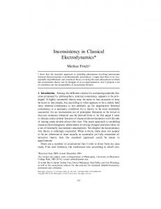
Now I can just make a fun little mathematica notebook which takes in stokes parameters and spits out plots!
a. b.
Linear Amplitude √ 3 5
Phase π 4 24 arccos( 25 )
Circular Aplitude √ 3 5
Phase arccos( √25 ) 0
3 1.0 2
0.5 1
-1.0
-0.5
0.5
-3
1.0
-2
-1
1
-1 -0.5 -2 -1.0 -3
Where the left figure depicts the field for part a. and the right figure for part b.
1
2
3
(11)
Zangwill 16.11 Consider two antipodal points on the Poincare Sphere describing fields with electric fields E and E 0 . We can choose to represent our fields in either the linear or circular polarization bases, I choose to use the linear basis. Then, saying that two points are antipodes on the poincare sphere means that s0 = s00 −→ s1 = s2 = s3 =
−s01 −s02 −s03
|�1 · E 0 |2 + |�2 · E 0 |2 = |�1 · E|2 + |�2 · E|2 0 2
−→ � −→
0 2
2
(12)
2
(13)
(�1 · E 0 )∗ (�2 · E 0 ) = −(�1 · E)∗ (�2 · E)
(14)
|�1 · E | − |�2 · E | = |�2 · E| − |�1 · E|
Armed with these relations, we press onwards. To determine the relative orientation of the E fields, in particular whether they are orthogonal, we shall copute their inner product. Recall that for complex vectors, the inner product is E 0∗ · E. The analysis is as follows E 0∗ · E = ((�1 · E 0 )�1 + (�2 · E 0 )�2 )∗ · ((�1 · E)�1 + (�2 · E)�2 ) = (�1 E 0 )∗ (�1 · E) + (�2 · E 0 )∗ (�2 · E) � � (�1 · E)∗ (�2 · E) = (�2 · E 0 )∗ (�2 · E) − (�1 · E) (�2 · E 0 ) � � �2 · E = (�2 · E 0 )∗ (�2 · E) − |�1 · E|2 �2 · E 0 � � �2 · E (|�1 · E 0 |2 − |�1 · E|2 − |�2 · E 0 |2 ) = (�2 · E 0 )∗ (�2 · E) + �2 · E 0
By equation 14
By equation 12
Note here that the first term cancels with the final part of the second term. That is, � � � � �2 · E �2 · E 0 2 |�2 · E | = (�2 · E 0 )∗ (�2 · E 0 ) = (�2 · E 0 )∗ (�2 · E) �2 · E 0 �2 · E 0 So that the term evaluated above and the first term in the expression of E 0∗ · E cancel. We now have the expression � � �2 · E (|�1 · E 0 |2 − |�1 · E|2 ) (15) E 0∗ · E = �2 · E 0 However, by adding equations 12 and 13 we get the expression 2|�1 · E 0 |2 = 2|�2 · E|2 → |�1 · E 0 |2 − |�1 · E|2 = 0
(16)
0∗
So, in fact, it is true that E · E = 0, or in other words antipodes on the poincare sphere represent orthogonal polarization states.
Zangwill 16.7 a. Consider the angular momentum of electromagnetic fields Z ~ EM = �0 d3 x ~r × (E ~ × B) ~ L
(17)
~ and introducing explicit indices we can write By introducing the vector potential in place of B ~ EM i = �0 L
Z Z
= �0 Z = �0
d3 x �ijk rj �klm El �mno ∂n Ao
(18)
d3 x (δkn δlo − δko δln )�ijk rj El ∂n Ao
(19)
d3 x (El �ijk rj ∂k Al − �ijk rj El ∂l Ak )
(20) (21)
2
The first term is exactly the Lorbital we are looking for. We can integrate the second term by parts, use the fact that these are sourceless fields so that ∂l El = 0 (this was stated in the original statement in Zangwill’s book) and use the fact that ∂l rj = δlj to write the second term as Z Z Z 3 3 ~ spin −�0 d x �ijk rj El ∂l Ak = �0 d x �ijk δlj El Ak = �0 d3 x �ijk Ej Ak = L (22) Thus, indeed the decomposition stated in the problem is correct.
b. Consider a gauge tranformation, A → A0 = A + ∇φ with φ a scalar function. Since the electric potential does not appear, we need not worry ourselves with it. Plugging this in
~0 EM = �0 L
Z
~ × (A ~ + ∇φ)) d3 x Ek (~r × ∇)(Ak + ∇k φ) + (E Z ~ EM + �0 d3 x Ek (~r × ∇)∇k φ + (E ~ × ∇φ) =L
(23) (24)
It is obvious that the second term will be nonzero in general, for example if we take φ to be a linear function of the coordinates, the first term is zero, but the second term will not in general be zero even with a linear function φ.
c. Consider a circularly polarized plane wave in the coloumb gauge ˆ ± iˆ y ~ ± = E0 x √ exp[i(kz − ωt)] E 2
(25)
In the coloumb gauge E = −∂t A → A = −i
E0 x ˆ ± iˆ y √ exp[i(kz − ωt)] ω 2
(26)
Consider the object
~ spin i = ±ωˆ ±ωˆ z · hL z h�0
Z
d3 x