Classical irregular block, N=2 pure gauge theory - arXiv

Classical irregular block, N “ 2 pure gauge theory and Mathieu equation Marcin Piatek a, c, 1

Artur R. Pietrykowski b, c, 2

a

Institute of Physics, University of Szczecin ul. Wielkopolska 15, 70-451 Szczecin, Poland b

arXiv:1407.0305v1 [hep-th] 1 Jul 2014

Institute of Theoretical Physics University of Wroclaw pl. M. Borna, 950-204 Wroclaw, Poland c

Bogoliubov Laboratory of Theoretical Physics, Joint Institute for Nuclear Research, 141980 Dubna, Russia

Abstract Combining the semiclassical/Nekrasov–Shatashvili limit of the AGT conjecture and the Bethe/gauge correspondence results in a triple correspondence which identifies classical conformal blocks with twisted superpotentials and then with Yang–Yang functions. In this paper the triple correspondence is studied in the simplest, yet not completely understood case of pure SU p2q super-Yang–Mills gauge theory. A missing element of that correspondence is identified with the classical irregular block. Explicit tests provide a convincing evidence that such a function exists. In particular, it has been shown that the classical irregular block can be recovered from classical blocks on the torus and sphere in suitably defined decoupling limits of classical external conformal weights. These limits are “classical analogues” of known decoupling limits for corresponding quantum blocks. An exact correspondence between the classical irregular block and the SU p2q gauge theory twisted superpotential has been obtained as a result of another consistency check. The latter determines the spectrum of the 2-particle periodic Toda (sin-Gordon) Hamiltonian in accord with the Bethe/gauge correspondence. An analogue of this statement is found entirely within 2d CFT. Namely, considering the classical limit of the null vector decoupling equation for the degenerate irregular block a celebrated Mathieu’s equation is obtained with an eigenvalue determined by the classical irregular block. As it has been checked this result reproduces a well known weak coupling expansion of Mathieu’s eigenvalue. Finally, yet another new formulae for Mathieu’s eigenvalue relating the latter to a solution of certain Bethe-like equation are found.

1 2

e-mail: [email protected] e-mail: [email protected]

1

Contents 1 Introduction

2

2 Quantum and classical irregular 2.1 Quantum irregular block . . . . 2.2 Classical irregular block . . . . 2.3 Decoupling limits . . . . . . .

blocks . . . . . . . . . . . . . . . . . . . . . . . . . . . . . . . . . . . . . . . . . . . . . . . . . . . . . . . . . . . . . . . . . . . . . . . . . . . . . . . . . . . . . . . . . . . . . . . . . . .

8 8 9 10

3 Mathieu equation in 2d CFT 3.1 Null vector equation for the degenerate irregular block . . . . . . . . . . . . . . . . . . . . 3.2 Classical limit . . . . . . . . . . . . . . . . . . . . . . . . . . . . . . . . . . . . . . . . . . .

12 12 14

4 Mathieu eigenvalue from N “ 2 gauge theory 4.1 Nekrasov–Shatashvili limit . . . . . . . . . . . . . . . 4.2 Saddle point equation . . . . . . . . . . . . . . . . . 4.3 Solution to saddle point equation . . . . . . . . . . . 4.4 Mathieu eigenvalue – contour integral representation

16 16 20 21 22

. . . .

. . . .

. . . .

. . . .

. . . .

. . . .

. . . .

. . . .

. . . .

. . . .

. . . .

. . . .

. . . .

. . . .

. . . .

. . . .

. . . .

. . . .

. . . .

. . . .

. . . .

5 Conclusions

25

A Appendices A.1 Expansion coefficients of 2d CFT and gauge theory functions . . . . . A.2 Ward identities . . . . . . . . . . . . . . . . . . . . . . . . . . . . . . . A.3 Mathieu eigenvalue from WKB . . . . . . . . . . . . . . . . . . . . . . A.4 Young diagrams, their profiles and Nekrasov partition function . . . . A.5 Product identities and Y functions . . . . . . . . . . . . . . . . . . . . A.6 The result of iterative solution of the saddle point equation for SU(2)

27 27 29 30 34 40 42

1

. . . . . .

. . . . . .

. . . . . .

. . . . . .

. . . . . .

. . . . . .

. . . . . .

. . . . . .

. . . . . .

. . . . . .

. . . . . .

Introduction

Studying the problem of the oscillations of an elliptical membrane E. Mathieu [1] obtained the following two ordinary differential equations with real coefficients [2, 3]:3

and

˘ d2 ψ ` ` λ ´ 2h2 cos 2x ψ “ 0, 2 dx ˘ d2 ψ ` ´ λ ´ 2h2 cosh 2x ψ “ 0 2 dx

i.e.

xPR

` ˘ d2 ψ ` λ ´ 2h2 cos 2ix ψ “ 0. 2 dpixq

(1.1)

(1.2)

In honor of their originator the eqs. (1.1), (1.2) are now called Mathieu and modified Mathieu equations respectively. As has been explicitly written down the modified Mathieu eq. (1.2) may be derived from eq. (1.1) by writing ix for x and vice versa. 3

In the present paper we adopt the notation from [4].

2

For certain λ and h2 there exists a general solution ψpxq of the eq. (1.1) and a Floquet exponent ν such that ψpx ` πq “ eiπν ψpxq. If ψ` pxq is the solution of the Mathieu equation satisfying the initial conditions ψ` p0q “ const. “ 1 p0q “ 0, the parameter ν can be determined from the relation [4]: a and ψ` cos πν “

ψ` pπq . a

(1.3)

Thus the Floquet exponent is determined by the value at x “ π of the solution ψ` pxq which is p0q even around x “ 0. To the lowest order (h2 “ 0) the even solution around x “ 0 is ψ` pxq “ ? ? a cos λx. Hence, from (1.3) for h2 “ 0 we have ν “ λ, and more in general ` ˘ ν 2 “ λ ` O h2 .

One can derive various terms of this expansion perturbatively. For instance, in the weak coupling regime, for small h2 , the eigenvalue λ as a function of ν and h2 explicitly reads as follows [4]: ` 2 ˘ 5ν ` 7 h8 h4 2 λ “ ν ` ` 2 pν 2 ´ 1q 32 pν 2 ´ 4q pν 2 ´ 1q3 `

`

˘ 9ν 4 ` 58ν 2 ` 29 h12

64 pν 2 ´ 9q pν 2 ´ 4q pν 2 ´ 1q5

` ˘ ` O h16 .

(1.4)

One sees that this expansion cannot hold for integer values of ν. These cases have to be dealt with separately, cf. [4]. The solutions of the (modified) Mathieu equation govern a vast number of problems in physics: (i) the propagation of electromagnetic waves along elliptical cylinder, (ii) the vibrations of a membrane in the shape of an ellipse with a rigid boundary (Mathieu’s problem) [2], (iii) the motion of a rod fixed on one end and being under periodic tension at the other end [3], (iv) the motion of particles in electromagnetic traps [5], (v) the inverted pendulum and the quantum pendulum, (vi) the wave scattering by D-brane [6], (vii) fluctuations of scalar field about a D3brane [7, 8], (viii) reheating process in inflationary models [9], (ix) determination of the mass spectrum of a scalar field in a world with latticized and circular continuum space [10], are just some of them. Eq. (1.1) can be looked at as a one-dimensional Schr¨ odinger equation Hψ “ Eψ with the 2 2 2 Hamiltonian (the Mathieu operator) H “ ´d {dx `2h cos 2x and the energy eigenvalue E “ λ. The Mathieu operator H belongs to the class of Schr¨ odinger operators with periodic potentials [11] which are of special importance in solid state physics. Mathieu’s equation has recently emerged in a fascinating context, namely in the studies of the interrelationships between quantum integrable systems (QIS), N “ 2 super-Yang–Mills (SYM) theories and two-dimensional conformal field theory (2d CFT). In order to spell out aims of the present work let us discuss certain aspects of these investigations in detail. First, recall

3

ˆ 2 ~´2 , 2x “ ϕ, i.e.: that eq. (1.1) with λ “ 8u~´2 , h2 “ 4Λ  „ 2 2 ~ B 2 ˆ ` Λ cos ϕ ψpϕq “ u ψpϕq ´ 2 Bϕ2

(1.5)

is a Schr¨ odinger equation for the quantum one-dimensional sine-Gordon system defined by the ˆ 2 cos ϕ. In this context quantities Λ, ˆ ϕ, u can be complex valued.4 Lagrangian L “ 12 ϕ9 2 ´ Λ Secondly, it is a well known fact that the (classical) sine-Gordon model encodes an information about the N “ 2 SU p2q pure gauge Seiberg–Witten theory [12]. More precisely, the so-called Bohr–Sommerfeld periods ¿ ¿ b 2 ˆ 2pu ´ Λ cos ϕq dϕ “: P0 pϕq dϕ ΠpΓq “ Γ

Γ

ˆ 2 cos ˘ϕ0 define for two complementary contours Γ “ A, B encircling the two turning points Λ the Seiberg–Witten system [13]: a “ ΠpAq, BFpaq{Ba “ ΠpBq.5 Here, a is a modulus and Fpaq denotes the Seiberg–Witten prepotential determining the low energy effective dynamics of the N “ 2 supersymmetric SU p2q pure gauge theory. As has been observed in [14] (see also [15, 16]) the above statement has its “quantum analogue” or “quantum generalization” which can be formulated as follows. Namely, the monodromies6 ¿ r ΠpΓq “ P pϕ, ~q dϕ Γ

of the exact WKB solution

ψpϕq “ exp

$ ϕ &i ż %~

P pρ, ~q dρ

, . -

7 r ˆ a, ~q{Ba “ ΠpBq. r BWpΛ, to the eq. (1.5) define the Nekrasov–Shatashvili system [17]: a “ ΠpAq, ˆ a, ~q “ Wpert pΛ, ˆ a, ~q ` Winst pΛ, ˆ a, ~q is the effective twisted superpotential of the Here, WpΛ, 2d SU p2q pure gauge (Ω-deformed) SYM theory defined in [17] as the following (Nekrasov– Shatashvili) limit ˆ a, ~q ” lim ǫ2 log ZpΛ, ˆ a, ǫ1“ ~, ǫ2 q WpΛ, ǫ2 Ñ0

ˆ a, ǫ1 , ǫ2 q “ Zpert pΛ, ˆ a, ǫ1 , ǫ2 qZinst pΛ, ˆ a, ǫ1 , ǫ2 q [19, 20]. of the Nekrasov partition function ZpΛ, Twisted superpotentials determine the low energy effective dynamics of the two-dimensional SYM theories restricted to the Ω-background. These quantities play also a pivotal role in the so-called Bethe/gauge correspondence [17, 21, 22, 23] that maps supersymmetric vacua of the N “ 2 theories to Bethe states of quantum integrable systems. A result of that duality is that 4

In other words we are dealing here with quantized integrable model defined on the complex plane which is not hermitian quantum-mechanical system. 5 Cf. appendix A.3. 6 Here, P pϕ, ~q “ P0 pϕq ` P1 pϕq~ ` P2 pϕq~2 ` . . .. 7 For SU pN q generalization of this result, see [18].

4

the twisted superpotentials are identified with the Yang–Yang functions [17] which describe the spectrum of the corresponding quantum integrable systems.8 Twisted superpotentials occur also in the context related to the AGT correspondence [24]. The AGT conjecture states that the Liouville field theory (LFT) correlators on the Riemann surface Cg,n with genus g and n punctures can be identified with the partition functions of a class Tg,n of four-dimensional N “ 2 supersymmetric SU p2q quiver gauge theories. A significant part of the AGT conjecture is an exact correspondence between the Virasoro blocks on Cg,n and the instanton sectors of the Nekrasov partition functions of the gauge theories Tg,n . Soon after its discovery, the AGT hypothesis has been extended to the SU pN q-gauge theories/conformal Toda correspondence [25]. The AGT duality works at the level of the quantum Liouville field theory. At this point arises a question, what happens if we proceed to the classical limit of the Liouville theory. This is the limit in which the central charge and the external and intermediate conformal weights of LFT correlators tend to infinity in such a way that their ratios are fixed. It is commonly believed that such limit exists and the Liouville correlation functions, and in particular, conformal blocks behave in this limit exponentially. It turns out that the semiclassical limit of the LFT correlation functions corresponds to the Nekrasov–Shatashvili limit (ǫ2 Ñ 0, ǫ1 “ const.) of the Nekrasov partition functions. A consequence of that correspondence is that the instanton parts of the effective twisted superpotentials can be identified with classical conformal blocks. Hence, joining together classical/Nekrasov–Shatashvili limit of the AGT duality and the Bethe/gauge correspondence one thus gets the triple correspondence which links the classical blocks to the twisted superpotentials and then to the Yang–Yang functions. The simplest, although not yet completely understood examples of that correspondence are listed below: classical block on 4-punctured sphere on 1-punctured torus ?

twisted superpotential SU p2q Nf “ 4 SU p2q N “

Yang–Yang function SLp2q-type Gaudin model

2˚

2-particle elliptic Calogero–Moser model

SU p2q pure gauge

2-particle periodic Toda chain

Our goals in this paper are twofold. First, we study the triple correspondence in case where the SYM theory is the SU p2q pure gauge theory (the third example above).9 We identify the question mark in the table above as the classical irregular block firr . The latter is the classical limit of the quantum irregular block Firr [27]. Motivations to study classical blocks were, for a long time, mainly confined to applications in pure mathematics, in particular, to the celebrated uniformization problem of Riemann surfaces [28, 29] which is closely related to the monodromy problem for certain ordinary differential equations [30, 31, 32, 33, 34, 35, 36, 37, 38].10 The importance of the classical blocks is not only limited to the uniformization theorem, but gives also information about the solution of the 8

The Yang–Yang functions are potentials for Bethe equations. For a discussion of the first example in the table above, see [26]. 10 In a somewhat different context, see also [39]. 9

5

Liouville equation on surfaces with punctures. Recently, a mathematical application of classical blocks emerged in the context of Painlev´e VI equation [40]. Due to the recent discoveries the classical blocks are also relevant for physics. Indeed, in addition to the correspondence discussed in the present paper lately the classical blocks have been of use to studies of the entanglement entropy within the AdS3 {2d CFT holography [41] and the topological string theory [42]. The second purpose of the present work is to discuss implications of the aforementioned triple correspondence for the eigenvalue problem of Mathieu’s operator. More concretely, as has been observed in [14] the eigenvalue u in eq. (1.5) (or equivalently λ in eq. (1.1)) can be found from r eq. a “ ΠpAq as a series in ~ by applying the exact WKB method. The result can be re-expressed ˆ a, ǫ1 q w.r.t. Λ. ˆ 11 The same “should as a logarithmic derivative of the twisted superpotential WpΛ, be visible” on the conformal field theory side. Indeed, Mathieu’s equation occurs entirely within formalism of 2d CFT as a classical limit of the null vector decoupling equation satisfied by the 3-point degenerate irregular block ( = matrix element of certain primary degenerate chiral vertex operator between Gaiotto states [27]). As expected, the eigenvalue in this equation is ˆ Concluding, these given by the logarithmic derivative of the classical irregular block firr w.r.t. Λ. observations pave the way for working out new methods for calculating Mathieu’s eigenvalues and eigenfunctions. The second goal of this paper is to check this possibility. Our studies of Mathieu’s equation and the classical irregular block are in particular motivated by recent results obtained by one of the authors in [37]. There have been derived novel expressions for the so-called accessory parameter B of the Lam´e equation:12 d2 η ´ rκ ℘pzq ` Bs η “ 0. dz 2 In particular, it has been found that Bpτ q κ d E2 pτ q, “ q ftorus p´κ, δ˚ ; qq ` 2 4π dq 12

(1.6)

where q “ expp2πiτ q and τ is a torus modular parameter; ftorus p ¨ , ¨ ; qq denotes the classical torus block.13 It is a well known fact that in a certain limit the Lam´e equation becomes the Mathieu equation. Hence, one may expect that the Lam´e equation with the eigenvalue expressed in terms of the classical torus block ftorus consistently reduces to the Mathieu equation with the eigenvalue given by the classical irregular block firr if in such a limit ftorus Ñ firr. If this statement is true it will give a strong evidence that conjectured formula (1.6) is correct. The organization of the paper is as follows. In section 2 we define the quantum irregular block Firr related to the SU p2q pure gauge Nakrasov instanton partition function, in accordance 11

See appendix A.3. Here, ℘pzq is the Weierstrass elliptic function and E2 pτ q denotes the second Eisenstein series. 13 In eq. (1.6) the classical torus block is evaluated on the so-called saddle point intermediate classical weight δ˚ “ 41 ` p2˚ , where p˚ is a solution of the following equation (p P R): ¸ ˜ c ˆ ˙ˇ B p3q 1 1 ˇ 2 S 2p, ´2i κ ` , 2p “ 2Rftorus ´κ, ` p ; q ˇ . Bp L 4 4 p“p˚ 12

Sp3q L is known classical Liouville action on the Riemann sphere with three hyperbolic singularities (holes), cf. [37].

6

with the so-called non-conformal AGT relation [27]. Inspired by the latter and the results of [17] we then conjecture that Firr exponentiates to the classical irregular block firr in the classical limit. Indeed, for the low orders of expansion of the quantum irregular block one can see that the classical limit of Firr exists yielding consistent definition of the classical irregular block. The latter corresponds to the twisted superpotential of the 2d N “ 2 SU p2q pure gauge theory. In addition, we perform another consistency checks suggesting that the function firr really “lives its own life”. In particular, we verify that classical blocks on the 1-punctured torus C1,1 and on the 4-punctured sphere C0,4 reduce to firr in certain properly defined decoupling limit of external classical weights. This limit is a classical analogue of known decoupling limits for quantum blocks on C1,1 and C0,4 . In section 3 (see also appendix A.2) we consider the classical limit of the null vector decoupling equation satisfied by the 3-point degenerate irregular block [16] and find an expression for the Mathieu eigenvalue. As has been already mentioned the latter is determined by the classical irregular block. This formula yields the well known weak coupling expansion (1.4) of the eigenvalue of the Mathieu operator. Section 4 is devoted to the derivation of the Mathieu eigenvalue from the non-conformal AGT counterpart of the classical irregular block, namely the twisted superpotential. The latter is obtained from the Nekrasov instanton partition function for pure SU p2q gauge theory as a zero limit in one of the two deformation parameters ǫ1 , ǫ2 . Since the Nekrasov partition function can be represented by the sum over profiles of the Young diagrams [19] (see appendix A.4 for details) the two deformation parameters are associated with two edges of elementary box of anisotropic Young diagrams. As a result the superpotential is obtained from the critical Young diagram which is determined by a dominating contribution to the partition function. The Mathieu eigenvalue can be thus found by means of the Bethe/gauge correspondence postulated in ref. [17]. In section 5 we present our conclusions. The problems that are still open and the possible extensions of the present work are discussed. In the appendix A.1 are collected formulae for expansion coefficients of 2d CFT and gauge theory functions used in the main text. In the appendix A.3 the Mathieu eigenvalue is obtained form the exact WKB method. Appendices A.4 and A.5 contain supplementary material to the section 4. Specifically, the Nekrasov partition function is given in terms of the profiles of the Young diagrams.

7

2

Quantum and classical irregular blocks

2.1

Quantum irregular block

In order to define the quantum irregular block first we will need to introduce the notion of the Gaiotto state. This is the vector | ∆, Λ2 y defined by the following conditions [27, 16]: ˆ ˙ Λ B 2 L0 | ∆, Λ y “ ∆` | ∆, Λ2 y, (2.1) 2 BΛ L1 | ∆, Λ2 y “ Λ2 | ∆, Λ2 y,

Ln | ∆, Λ2 y “ 0

(2.2)

@ n ě 2.

(2.3)

In [43] it was shown that the state | ∆, Λ2 y which solves the Gaiotto constraint equations has the following form ÿ “ ÿ ÿ ‰p1n qJ Gnc,∆ | ∆, Λ2 y “ Λ2n | ∆, n y “ Λ2n L´J | ∆ y. (2.4) n“0

n“0

|J|“n

ı ıIJ ” ” “ x ∆ |LI L´J | ∆ y in the denotes the inverse of the Gram matrix Gnc,∆ Above Gnc,∆ IJ standard basis | ∆, J y :“ L´J | ∆ y “ L´k1 . . . L´kn | ∆ y,

J “ pk1 ě . . . ě kn ě 1q ,

(2.5)

|J| “ kn ` . . . ` k1 “ n of the Verma module with the central charge c and the highest weight ∆. The quantum irregular block is defined as the scalar product x ∆, Λ2 | ∆, Λ2 y of the Gaiotto state. Hence, taking into account (2.4) one gets14 ÿ ÿ “ ‰p1n qp1n q x ∆, Λ2 | ∆, Λ2 y “ Λ4n x ∆, n | ∆, n y “ Λ4n Gnc,∆ . (2.6) n“0

n“0

Due to the AGT relation the irregular block can be expressed through the SU p2q pure gauge Nf “0,SUp2q . Indeed, the following relation Nekrasov instanton partition function Zinst ÿ “ ‰p1n qp1n q Fc,∆ pΛq :“ x ∆, Λ2 | ∆, Λ2 y “ Λ4n Gnc,∆ “

ÿ

n“0

ˆ 4n

Λ

n“0

N “0,SUp2q

f Zn pa, ǫ1 , ǫ2 q “ Zinst

ˆ a, ǫ1 , ǫ2 q pΛ,

(2.7)

holds for ˆ Λ Λ “ ? , ǫ1 ǫ2 where

pǫ1 ` ǫ2 q2 ´ 4a2 ∆ “ , 4ǫ1 ǫ2 1 Q “ b` ” b

c

ǫ2 ` ǫ1

c “ 1`6 c

ǫ1 ǫ2

ô

ˆ

b “

ǫ1 ` ǫ2 ? ǫ1 ǫ2 c

˙2

ǫ2 . ǫ1

” 1 ` 6Q2 ,

(2.8)

(2.9)

For a non rigorous derivation of eq. (2.7), see [44]. Rigorous proof can be found in ref. [45]. 14

For an explicit computation of the first few coefficients in (2.6), see appendix A.1.

8

2.2

Classical irregular block

In [17] it was observed that in the limit ǫ2 Ñ 0 the Nekrasov partition functions behave exponentially. In particular, for the instantonic sector we have * " 1 ǫ2 Ñ0 Nf “0,SUp2q ˆ Nf “0,SUp2q ˆ W pΛ, a, ǫ1 q . (2.10) Zinst pΛ, a, ǫ1 , ǫ2 q „ exp ǫ2 inst In other words, there exists the limit N “0,SUp2q

f Winst

N “0,SUp2q

ˆ a, ǫ1 q ” lim ǫ2 log Z f pΛ, inst ǫ2 Ñ0

“

ÿ

k“1

ˆ 4k Wk pa, ǫ1 q Λ

(2.11)

called the effective twisted superpotential. Taking into account (2.7), (2.8), (2.9) and (2.10) one can expect the exponential behaviour a ˆ 1 bq, c “ 1 ` 6Q2 , of the irregular block in the limit b Ñ 0. Indeed, let b “ ǫ2 {ǫ1 and Λ “ Λ{pǫ ∆ “ b12 δ, δ “ Opb0 q then, we conjecture that ˜ ¸+ # ˆ Λ 1 bÑ0 . (2.12) Fc,∆ pΛq “ x ∆, Λ2 | ∆, Λ2 y „ exp 2 fδ b ǫ1 Equivalently, there exists the limit » fi ˜ ¸ ˜ ¸ ˜ ¸4n ÿ ˆ ˆ ˆ “ n ‰p1n qp1n q Λ Λ Λ fl “ lim b2 log Fc,∆ fδ “ lim b2 log –1 ` Gc,∆ bÑ0 bÑ0 ǫ1 ǫ1 b ǫ b 1 n“1 ˜ ¸4n ÿ Λ ˆ fδn (2.13) “ ǫ 1 n“1 called the classical irregular block. It should be stressed that the asymptotical behaviuor (2.12) is a nontrivial statement concerning the quantum irregular block. Although there is no proof of this property the existence of the classical irregular block can be checked, first, by direct calculation. For instance, up to n “ 3 one finds fδ1 “

1 , 2δ

fδ2 “

5δ ´ 3 , 16δ3 p4δ ` 3q

fδ3 “

9δ2 ´ 19δ ` 6 . 48δ5 p4δ2 ` 11δ ` 6q

(2.14)

ˆ 1 q. As has been shown Secondly, there exist two other equivalent ways to get the function fδ pΛ{ǫ in ref. [43] the irregular block Fc,∆ pΛq can be recovered from the 4-point block on the ı ” quantum ∆3 ∆2 sphere Fc,∆ ∆4 ∆1 pxq in a properly defined decoupling limit of the external conformal weights ∆i ,15 ı ” µ1 ,µ2 ,µ3 ,µ4 Ñ 8 3 ∆2 (2.15) F˜c,∆ ∆ ∆4 ∆1 pxq ÝÝÝÝÝÝÝÝÝÝÑ Fc,∆ pΛq, ˆ4 xµ1 µ2 µ3 µ4 “Λ

where (ǫ “ ǫ1 ` ǫ2 ):

pǫ ` µ3 ´ µ4 q pǫ ´ µ3 ` µ4 q , 4ǫ1 ǫ2 pǫ ` µ1 ´ µ2 q pǫ ´ µ1 ` µ2 q , ∆2 “ 4ǫ1 ǫ2

pµ3 ` µ4 q p2ǫ ´ µ3 ´ µ4 q , 4ǫ1 ǫ2 pµ1 ` µ2 q p2ǫ ´ µ1 ´ µ2 q ∆1 “ . 4ǫ1 ǫ2

∆4 “

15

∆3 “

ˆ 1 bq. Here and below, Λ “ Λ{pǫ

9

(2.16)

˜

∆ pqq with The same phenomenon occurs in the case of the 1-point block on the torus Fc,∆

˜ “ rm pǫ1 ` ǫ2 ´ mqs{pǫ1 ǫ2 q. ∆

(2.17)

˜ [46], The torus 1-point block yields Fc,∆ pΛq after a decoupling of the external weight ∆ ˜ mÑ8 ∆ pqq ÝÝÝÝÝÑ Fc,∆ pΛq. F˜c,∆ ˆ4 qm4 “Λ

(2.18)

Our claim is that the decoupling limits (2.15), (2.18) work also on ”the “classical level”, i.e. after ı ˜ ∆3 ∆2 ∆ pqq. We taking the classical limit of the quantum conformal blocks Fc,∆ ∆4 ∆1 pxq and Fc,∆ describe this observation in detail in the next subsection.

2.3

Decoupling limits

As a starting point let us recall definitions of the 4-point block on the sphere and the 1-point block on the torus. Let x be the modular parameter of the 4-punctured Riemann sphere then the s-channel conformal block on C0,4 is defined as the following formal x-expansion: ¸ ˜ 8 ı ” ı ” ÿ n n ∆3 ∆2 ∆´∆2 ´∆1 3 ∆2 Fc,∆ 1` Fc,∆ ∆ ∆4 ∆1 x ∆4 ∆1 pxq “ x n Fc,∆

”

∆3 ∆2 ∆4 ∆1

ı

“: x “

∆´∆2 ´∆1

lim

zÑ1

”

n“1

3 ∆2 F˜c,∆ ∆ ∆4 ∆1

ÿ

n“|I|“|J|

ı

pxq,

ıIJ ” x ∆4 | V∆3 pzq |∆, I y Gc,∆ x ∆, J | V∆2 pzq | ∆1 y .

Let q “ e2πiτ be the elliptic variable on the torus with modular parameter τ then the conformal block on C1,1 is given by the following formal q-series: ¸ ˜ 8 ÿ c ˜ ˜ ∆,n ∆ pqq “ q ∆´ 24 1 ` Fc,∆ Fc,∆ q n n“1

˜

∆,n Fc,∆

“: q “

c ∆´ 24

lim

zÑ1

˜ ∆ F˜c,∆ pqq, ıIJ ÿ @ D ” Gc,∆ . ∆, I | V∆ ˜ pzq |∆, J

n“|I|“|J|

Above appear the matrix elements of the primary chiral vertex operator between the basis states (2.5). In order to calculate them it is sufficient to know: piq the covariance properties of the primary chiral vertex operator w.r.t. the Virasoro algebra, ˙ ˆ d n rLn , V∆ pzqs “ z z ` pn ` 1q∆ V∆ pzq , n P Z; dz piiq the form of the normalized matrix element of the primary chiral vertex operator,16 @ D ∆i | V∆j pzq | ∆k “ z ∆i ´∆j ´∆k . 16

The normalization condition takes the form

@

∆i | V∆j p1q | ∆k

10

D

“ 1.

Let us consider the classical limit of conformal blocks, i.e. the limit in which the central charge c “ 1 ` 6pb ` 1b q2 , external and intermediate conformal weights tend to infinity in such a way that their ratios are fixed. It is known (however not yet proved) that in such limit quantum conformal blocks exponentiate. In particular, for conformal blocks on C0,4 and C1,1 we have " * ı ” 1 ”δ3 δ2 ı bÑ0 3 ∆2 pxq „ exp F˜c,∆ ∆ f pxq , (2.19) δ δ4 δ1 ∆4 ∆1 b2 " * 1 δ˜ ˜ bÑ0 ∆ ˜ Fc,∆ pqq „ exp 2 fδ pqq . (2.20) b Above it is assumed that the quantum conformal weights are heavy: ∆i “

1 δi , b2

˜ ˜ “ 1 δ, ∆ b2

∆ “

1 δ, b2

˜ δ “ Opb0 q. δi , δ,

The functions: ”

fδ δδ34 δδ21

ı

pxq “

8 ÿ

”

fδn δδ34 δδ21

n“1

ı

˜ fδδ pqq

n

x ,

“

8 ÿ

˜

fδδ,n q n

n“1

are known as the classical conformal the sphere [30, 47, 48] and on the torus [37] ” ıblocks on ˜ δ,n δ3 δ2 n respectively. The coefficients fδ δ4 δ1 and fδ can be found directly from the semiclassical asymptotics (2.19), (2.20) and the power expansions of quantum blocks: ¸ ˜ 8 8 ı ” ” ı ÿ ÿ n n ∆3 ∆2 n 2 n δ3 δ2 Fc,∆ ∆4 ∆1 x , fδ δ4 δ1 x “ lim b log 1 ` bÑ0

n“1

8 ÿ

n“1

˜ fδδ,n q n

n“1

˜

2

“ lim b log 1 ` bÑ0

8 ÿ

˜ ∆,n Fc,∆

q

n

n“1

¸

,

see appendix A.1. Let us observe that the quantum external weights (2.16), (2.17) are heavy in the terminology of [30], i.e. exist the limits: ǫ2 ∆i , ǫ2 Ñ0 ǫ1

˜ ˜ “ lim ǫ2 ∆. δ˜ “ lim b2 ∆ ǫ2 Ñ0 ǫ1 bÑ0

δi “ lim b2 ∆i “ lim bÑ0

The classical external weights explicitly read as follows “ ‰ ` ˘ ` ˘ δ4 “ ǫ21 ´ pµ3 ´ µ4 q 2 { 4ǫ21 , δ3 “ rpµ3 ` µ4 q p2ǫ1 ´ µ3 ´ µ4 qs { 4ǫ21 , “ ‰ ` ˘ ` ˘ δ2 “ ǫ21 ´ pµ1 ´ µ2 q 2 { 4ǫ21 , δ1 “ rpµ1 ` µ2 q p2ǫ1 ´ µ1 ´ µ2 qs { 4ǫ21

(2.21)

and

δ˜ “ rm pǫ1 ´ mqs {ǫ21 . Hence, one can consider the b Ñ 0 limit of both sides of the decoupling limits (2.15), (2.18). Then, for the classical weights given by (2.21) one can verify order by order that ” ı µ1 ,µ2 ,µ3 ,µ4 Ñ 8 ˆ 1 q, fδ δδ34 δδ21 pxq ÝÝÝÝÝÝÝÝÝÝÑ fδ pΛ{ǫ ˆ4 xµ1 µ2 µ3 µ4 “Λ

˜ fδδ pqq

mÑ8

ÝÝÝÝÝÑ ˆ4 qm4 “Λ

11

ˆ 1 q. fδ pΛ{ǫ

F˜c,∆

”

∆3 ∆2 ∆4 ∆1

ı

pxq

∆i Ñ 8

δ3 δ2 δ4 δ1

ı pxq

δi Ñ 8

˜ ∆ F˜c,∆ pqq

bÑ0

bÑ0

”

˜ Ñ8 ∆

ˆ 1 bq Λ “ Λ{pǫ

bÑ0 exp b12 fδ

Fc,∆ pΛq

ˆ 1q exp b12 fδ pΛ{ǫ

δ˜ Ñ 8

˜

exp b12 fδδ pqq

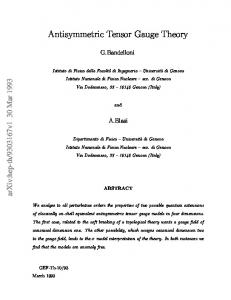
ˆ 1 q (above Figure 1: Equivalent ways to get the classical irregular block fδ pΛ{ǫ 1 1 2 ˜ ˜ c “ 1 ` 6pb ` b q and p∆, ∆i , ∆q “ b2 pδ, δi , δqq.

Calculations presented above can be visualized on the diagram (see fig.1). Let us stress that the commutativity of this diagram lend a strong support to the exponentiation hypothesis (2.12), (2.19), (2.20) of conformal blocks in the limit b Ñ 0. As a final remark in this section let us observe that joining together (2.7)-(2.9), (2.10) and (2.12) one gets ˆ 1 q “ 1 W Nf “0,SUp2q pΛ, ˆ a, ǫ1 q, fδ pΛ{ǫ (2.22) ǫ1 inst where

ǫ2 1 a2 ∆ “ ´ 2. ǫ2 Ñ0 ǫ1 4 ǫ1

δ “ lim b2 ∆ “ lim bÑ0

(2.23)

Indeed, to show the consistency of our approach one can use (2.14) and formulae from the appendix A.1, and check that 1 1 WnNf “0,SUp2q “ 4n f n1 a2 , ǫ1 ǫ1 4 ´ ǫ2 1

3 3.1

n “ 1, 2, 3, . . . .

(2.24)

Mathieu equation in 2d CFT Null vector equation for the degenerate irregular block

Let

1 3 ∆ ` “ ´ ´ b2 2 4 denotes the degenerate primary chiral vertex operator [49] V` pzq ” V∆` pzq,

˜ ∆1 ∆` ∆ z 0 p| ∆` y

V` pzq ” V 8

b ¨ q : V∆ ˜ Ñ V ∆1

˜ acting between the Verma modules V∆ ˜ and V∆1 . We will assume that the conformal weights ∆ and ∆1 are related by the fusion rule, i.e.: ˆ ˙ ˆ ˙ b b Q2 1 ˜ “ ∆ σ´ ∆ ´ σ2. (3.1) , ∆ “ ∆ σ` , where ∆pσq “ 4 4 4 12

Let us consider the descendant17

„ p ´2 pzq ´ χ` pzq “ L

3 2p2∆` ` 1q

 2 p L´1 pzq V` pzq

of V` pzq which corresponds to the null vector appearing on the second level of the Verma module V∆` . According to the null vector decoupling theorem [51] (see also [52]) the matrix element of χ` pzq, between the states with the highest weights obeying (3.1), must vanish. In particular, vanishes the matrix element ˜ Λ2 y “ x ∆1 , Λ2 | L p ´2 pzqV` pzq | ∆, ˜ Λ2 y x ∆1 , Λ2 | χ` pzq | ∆, 1 p2´1 pzqV` pzq | ∆, ˜ Λ2 y “ 0, ` 2 x ∆1 , Λ2 | L b ˜ Λ2 y are the Gaiotto states introduced in (2.1)-(2.3). The above null where x ∆1 , Λ2 | and | ∆, vector decoupling condition can be converted to the following partial differential equation for ˜ Λ2 y [16], the degenerate irregular 3-point block ΨpΛ, zq “ x ∆1 , Λ2 |V` pzq| ∆, « ff ˆ ˙ ˜ ` ∆1 ´ ∆` 1 2 B2 B ∆ 3z B 1 Λ ΨpΛ, zq “ 0 . (3.3) ` Λ2 z ` ` z ´ ` b2 Bz 2 2 Bz z 4 BΛ 2 Indeed, using the Ward identity

where T pwq “ one can find

2

ř

nPZ w

´n´2 L

n

„

ˆ 2 ˙ z B Λ ∆` Λ2 ` ` 3 ` wpw ´ zq Bz pw ´ zq2 w w ˆ ˙ 1 Λ B B ˜ ` ∆1 ´ ∆` ´ z ` `∆ ΨpΛ, zq, 2w2 2 BΛ Bz

˜ Λ2 y “ x ∆ , Λ | T pwqV` pzq | ∆, 1

(3.4)

is the holomorphic component of the energy-momentum tensor,

ˆ 2 ˙ Λ Λ2 1 B ` ` 3 ´ z Bz z z ˆ ˙ 1 Λ B ˜ ` ∆1 ´ ∆` ´ z B ` 2 `∆ ΨpΛ, zq, (3.5) 2z 2 BΛ Bz 2 p 2 pzqV` pzq | ∆, ˜ Λ2 y “ B ΨpΛ, zq. x ∆1 , Λ2 | L (3.6) ´1 Bz 2 For a derivation of eqs. (3.4), (3.5), see appendix A.2. At this point, a few comments concerning ΨpΛ, zq are necessary. First, let us note that from (2.4) we have ˜ ÿ ˜ Λ2 y “ z ∆1 ´∆` ´∆ Λ2pm`nq z m´n ΨpΛ, zq “ x ∆1 , Λ2 |V` pzq| ∆, „

p ´2 pzqV` pzq | ∆, ˜ Λ2 y “ x∆ ,Λ |L 1

2

m,ně0

ˆ

ÿ

ÿ “

Gm c,∆1

|I|“m |J|“n

‰p1m qI

ıJp1n q ” ˜ J y Gn ˜ x ∆1 , I | V` p1q | ∆, c,∆

” z κ ΦpΛ, zq, 17

(3.8)

Recall that [50] p ´k pzq ” L

(3.7)

1 2πi

¿

dwpw ´ zq1´k T pwq.

Cz

13

(3.2)

˜ where κ ” ∆1 ´ ∆` ´ ∆. Let us observe that Φpz, Λq can be split into two parts, i.e. when m “ n and m ‰ n: ΦpΛ, zq “ Φpm“nq pΛq ` Φpm‰nq pΛ, zq, ıIp1n q ” ÿ “ ÿ ‰p1n qI ˜ I y Gn ˜ x ∆1 , I | V` p1q | ∆, , Gnc,∆1 Φpm“nq pΛq “ Λ4n c,∆ ně0

Φpm‰nq pΛ, zq “

ÿ

(3.9)

|I|“n

Λ2pm`nq z m´n

ÿ

|I|“m, |J|“n

m‰n m,ně0

“

Gm c,∆1

‰p1m qI

ıJp1n q ” ˜ J y Gn ˜ x ∆1 , I | V` p1q | ∆, . c,∆

Then, one can write ! ´ ¯) ΨpΛ, zq “ z κ exp log Φpm“nq pΛq ` Φpm‰nq pΛ, zq (3.10) ¸+ # ˜ Φpm‰nq pΛ, zq ” z κ eφ1 pΛq eφ2 pΛ,zq . “ z κ exp log Φpm“nq pΛq ` log 1 ` Φpm“nq pΛq Inserting (3.8) into the eq. (3.3) we get „ ˆ ˙ 1 2 2 2κ 3 κpκ ´ 1q 3κ Λ z Bz ` ´ ´ zBz ` BΛ ` 2 2 b b 2 4 b2 2 ff ˙ ˜ ˆ 1´∆ ∆ ` ∆ 1 ` ΦpΛ, zq “ 0. (3.11) ` Λ2 z ` ` z 2

3.2

Classical limit

Now, we want to find the limit b Ñ 0 of the eq. (3.11). This firstly requires to rescale the ˜ and ∆1 , i.e. σ “ ξ{b and to express Λ as Λ “ Λ{pǫ ˆ 1 bq. After rescaling we have parameter σ in ∆ bÑ0

˜ „ ∆1 , ∆

1 δ, b2

where

1 ˜ ` ∆1 ´ ∆` bÑ0 ∆ „ 22 b bÑ0

κ ÝÑ

1 ´ ξ, 2

ˆ

˜ “ δ “ lim b2 ∆1 “ lim b2 ∆ bÑ0

1 ´ ξ2 4

˙

bÑ0

1 2δ, b2 ˆ ˙ 1 bÑ0 2 κ pκ ´ 1q ÝÑ ´ ´ξ “ ´δ. 4 “

1 ´ ξ2, 4

(3.12) (3.13) (3.14)

bÑ0

Note, that ∆` „ Opb0 q. Secondly, one has to determine the behavior of the normalized degenerate irregular block ˆ 1 bq and ∆1 , ∆ ˜ bÑ0 Φ “ z ´κ Ψ when b Ñ 0. For Λ “ Λ{pǫ „ b12 δ it is reasonable to expect, that " * 1 bÑ0 ´κ 1 2 2 ˜ Λ y „ vpΛ{ǫ ˆ 1 , zq exp ˆ 1q , ΦpΛ, zq “ z x ∆ , Λ | V` pzq | ∆, fδ pΛ{ǫ (3.15) b2 where (cf. (3.10)) ˆ 1 , zq “ lim eφ2 pΛ,zq “ elimbÑ0 φ2 pΛ,zq , vpΛ{ǫ bÑ0

ˆ 1 q “ lim b2 φ1 pΛq “ lim b2 log Φpm“nq pΛq . fδ pΛ{ǫ bÑ0

bÑ0

14

(3.16) (3.17)

Let us stress that the asymptotic (3.15) is a nontrivial statement concerning the 3-point irregular block ΦpΛ, zq. We have no rigorous proof of this conjecture. However, the eq. (3.15) can be well confirmed by direct calculations. Indeed, one can check order by order that the limits (3.16) and (3.17) exist. Moreover, the latter yields the classical irregular block. Then, after substituting (3.15) into the eq. (3.11), multiplying by b2 , and taking the limit b Ñ 0 one gets18 « ff ˙ ˆ ˆ2 ˆ Λ Λ 1 ˆ 1 q vpzq “ 0 . z 2 Bz2 ` 2p 12 ´ ξqzBz ` 2 z ` (3.18) ` BΛˆ fδ pΛ{ǫ z 4 ǫ1 In order to get the Mathieu equation we define a new function ψpzq related to the old one by vpzq “ z ξ ψpzq. Now, what we obtain equals «

ff ˙ ˆ ˆ2 ˆ Λ 1 Λ 2 ˆ 1 q ´ ξ ψpzq “ 0 . (3.19) ` BΛˆ fδ pΛ{ǫ ` zBz ` 2 z ` z 4 ǫ1 ˘ ` 2 ψ pew q then, the eq. (3.19) Since for z “ ew the derivatives transform as z 2 Bz2 ` zBz ψpzq “ Bw goes over to the form « ff ˆ2 ˆ d2 Λ Λ 2 ˆ 1 q ´ ξ ψ pew q “ 0. (3.20) ` 2 2 coshpwq ` BΛˆ fδ pΛ{ǫ dw2 4 ǫ1 z 2 Bz2

Finally, the substitution w “ 2ix, x P R in (3.20) yields ff « ˆ2 Λ d2 2 ˆ B ˆ fδ pΛ{ǫ ˆ 1 q ´ 4ξ ψpe2ix q “ 0. ´ 2 ` 8 2 cos 2x ` Λ Λ dx ǫ1

(3.21)

Now, one can identify the parameters λ and h appearing in the Mathieu equation (1.1) as follows ´ ¯ ˆ B ˆ fδ Λ{ǫ ˆ 1 ` 4ξ 2 , λ “ ´Λ Λ

h “ ˘

ˆ 2Λ . ǫ1

(3.22)

Let us observe that using (2.14) and postulating the following relation ξ “

ν 2

between the parameter ξ and the Floquet exponent ν one finds « ff ¯4n ÿ´ n ˆ 1 f ` 4ξ 2 ˆ Bˆ Λ{ǫ λ “ ´Λ

(3.23)

δ

Λ

n“1

4h4 1 8h8 2 12h12 3 “ ´ f 1 ν2 ´ f 1 ν2 ´ f 2 ´ ... ` 4 16 4 ´ 4 256 4 ´ 4 4096 41 ´ ν4

ˆ

ν2 4

˙

` 4 ˘ ` 2 ˘ 9ν ` 58ν 2 ` 29 h12 5ν ` 7 h8 h4 “ ν ` ` ` ... . ` 2 pν 2 ´ 1q 32 pν 2 ´ 4q pν 2 ´ 1q3 64 pν 2 ´ 9q pν 2 ´ 4q pν 2 ´ 1q5 2

18

ˆ

The key point here is the fact that limbÑ0 b2 Λ4 BΛˆ v “ 0.

15

Hence, the formula (3.22) reproduces the expansion (1.4). On the other hand one can check that the formula (3.22) exactly matches that obtained by means of the WKB method. Indeed, taking into account that (cf. (2.23)) δ “

1 a2 1 ´ 2 “ ´ ξ2 4 4 ǫ1

ðñ

ξ“

a ǫ1

one can rewrite the eq. (3.21) to the following Schr¨ odinger-like form: „  2 2 d 2 ˆ ´ǫ1 2 ` 8Λ cos 2x ψ “ E ψ, dx

(3.24)

where ˆ 1 q. ˆ B ˆ f 1 a2 pΛ{ǫ E “ ǫ21 λ “ 4a2 ´ ǫ21 Λ Λ ´ 4

(3.25)

ǫ2 1

The “energy eigenvalue” E in eq. (3.24) can be computed by making use of the WKB method. These calculations are performed in the appendix A.3. The result of the WKB calculations coincides with E given by eq. (3.25). This check is yet another example of an interesting link between the semiclassical limit of conformal blocks and the WKB approximation.

4

Mathieu eigenvalue from N “ 2 gauge theory

We saw in previous sections that the eigenvalue of the Mathieu operator is related to the classical irregular conformal block. The latter appeared to be a limit of the quantum irregular conformal block when b2 „ ~ Ñ 0. The irregular quantum conformal block is found to be related [43] to the Nekrasov’s instanton partition function of the pure (Nf “ 0) N “ 2 SYM. Nekrasov’s partition function in the zero limit of one of its parameters (in what follows we take it to be ǫ2 ) yields an effective twisted superpotential. Therefore it is natural to expect that thus established correspondence between the two theories at the quantum level also extends to the classical level. In the preceding section we found a relation between the expansion parameters Nf “0,SUp2q ˆ pΛ{ǫ1 , a, bq and verified the agreement on both sides of the correspondence Fc,∆ pΛq “ Zinst between expansion coefficients of classical irregular block and twisted superpotential up to the third order. In this section we address the derivation of the twisted superpotential W from the representation of the instanton partition function for N “ 2 pure gauge SYM in terms of profile functions of the Young diagrams employed in this context first by Nekrasov and Okounkov [19].

4.1

Nekrasov–Shatashvili limit

The Nekrasov’s partition function for N “ 2 pure SYM with SU pN q symmetry on Ω-background relates instanton configurations on a moduli space with partitions a graphical representation of whose are Young diagrams. This relationship makes the mentioned gauge theory tantamount to the theory of random partitions. There are five equivalent forms of the instanton partition function (see appendix A.4 for notation and more information about Nekrasov partition function).

16

For our purpose we use the following one $ , & ÿ . Nf “0,SUpNq ˆ ˆ a, ǫ1 , ǫ2 q “ exp ´ ˆ Z Nf “0,SUpNq pΛ, γǫ1 ,ǫ2 paα ´ aβ ; Λq pΛ, a, ǫ1 , ǫ2 q, Zinst % -

(4.1a)

α,β“1

where the first factor on the right hand side is a perturbative part. The second is defined as follows ˜ ¸2N k ÿ Λ ˆ Nf “0,SUpNq ˆ Zk pa, ǫ1 , ǫ2 q, (4.1b) Zinst pΛ, a, ǫ1 , ǫ2 q ” ǫ1 kě0 ¯ ` ´1 ˘ ´ ´1 0 0 q Γ ǫ px ´ x ´ ǫ q Γ ǫ px ´ x ź ÿ α,i 1 β,j α,i 2 2 β,j ¯. Zk pa, ǫ1 , ǫ2 q ” b´4N k (4.1c) ` ´1 ˘ ´ ´1 0 0 ´ǫ q Γ ǫ px ´ x q Γ ǫ px ´ x α,i 1 β,j pα,iq‰pβ,jq k:|k|“k 2 2 α,i β,j

The arguments of the Euler gamma functions are defined as follows19 xα,i ” aα ` ǫ1 pi ´ 1q ` ǫ2 kαi ,

x0α,i ” aα ` ǫ1 pi ´ 1q.

(4.2)

Thus, the instatnon partition function is expressed in terms of partitions of an integer instanton ř ř number k i.e., k “ |k| “ |kα | “ kα,i , α “ 1, . . . , N and i P N, such that for any i ă j and fixed α, kα,i ě kα,j ě 0. This particular form of it is related to the one, defined in terms of the profiles of the deformed Young diagrams. Namely, ˆ a, ǫ1 , ǫ2 q Z Nf “0,SUpNq pΛ, “

ÿ

fa,k PPpYN q

, $ . & 1ij 2 2 ˆ exp ´ ´´ dxdy fa,k px|ǫ1 , ǫ2 qγǫ1 ,ǫ2 px ´ y; Λqfa,k py|ǫ1 , ǫ2 q , (4.3) % 4 R2

where PpYN q denotes the space of all profiles of N -tuple of Young diagrams. The profile function is defined as follows20 fa,k px|ǫ1 , ǫ2 q ”

N ÿ

α“1

|x ´ aα | `

N ÿ ´ˇ ÿ ˇ ˇx ´ x0 ´ ǫ1 ˇ ´ |x ´ xα,i ´ ǫ1 | α,i

α“1 iě1

¯ ˇ ˇ ´ ˇx ´ x0α,i ˇ ` |x ´ xα,i | . (4.4)

In what follows we work with the instanton density rather then with the profile functions. The linear density function of instantons at position a and configuration k is defined as ρa,k px|ǫ1 , ǫ2 q ” fa,kpx|ǫ1 , ǫ2 q ´ fa,H px|ǫ1 , ǫ2 q, 19

(4.5)

More precisely, the point xα,i is a coordinate of ith column within a αth Young diagram depicted in the Russian convention and projected onto the real axis. The relation of the Russian convention of drawing a Young diagram to e.g., the English one boils down to rotation of the latter by 135˝ about its pivot point aα . In this case the decline of columns coincides with the linear order of R. Since ǫ1 ‰ ǫ2 the boxes of a Young diagram are ? deformed to rectangles with edges li “ 2|ǫi |, i “ 1, 2. 20 Note, that this definition of the profile function, when defined for real argument, is meaningful if and only if both parameters ǫ1 or ǫ2 have opposite signs.

17

where the second term is the empty profile given by the first term on the right hand side of eq. (4.4). The instanton density satisfies the following normalization condition ż 1 dx ρa,k px|ǫ1 , ǫ2 q. (4.6) k“ ´2ǫ1 ǫ2 R

The above equation shows that the density function stores the information about both, the number of instantons and their configuration. The partition function expressed in terms of profiles in eq. (4.3) can now be written in terms of instanton densities. Discarding the perturbative part which takes the form of the multiplier in eq. (4.1a) the instatnon part reads ! ) ÿ Nf “0,SUpNq ˆ ˆ , pΛ, a, ǫ1 , ǫ2 q “ exp ´Hinst rρa,k spǫ1 , ǫ2 , Λq (4.7) Zinst ρa,k PRpYN q

where RpYN q ĂPpYN q.21 The Hamiltonian for instanton configurations structurally reads ˆ ” 1 pf 2 qi γǫ ,ǫ pΛq ˆ ij pρ2 qj ` 1 pρ2 qi γǫ ,ǫ pΛq ˆ ij pf 2 qj Hinst rρa,k spǫ1 , ǫ2 , Λq 1 2 k 1 2 H 4 H 4 k

ˆ ij pρ2 qj . (4.8) ` 41 pρ2k qi γǫ1 ,ǫ2 pΛq k

In the above equation we introduced the following notation ij 2 j 2 i ˆ 2 py|ǫ1 , ǫ2 q. ˆ pρk q γǫ1 ,ǫ2 pΛqij pρk q ” ´´ dxdy ρ2a,k px|ǫ1 , ǫ2 qγǫ1 ,ǫ2 px ´ y; Λqρ a,k

(4.9)

R2

In what follows we are concerned with the form of the instanton partition within the NekrasovShatashvili limit i.e., when one of the deformation parameters tends to zero. This limit of the Nekrasov partition function defines the effective twisted superpotential. Explicitly ˆ a, ǫ1 q ” ´ lim ǫ2 log Z Nf “0,SUpNq pΛ, ˆ a, ǫ1 , ǫ2 q, W Nf “0,SUpNq pΛ, ǫ2 Ñ0

(4.10)

where W “ Wpert ` Winst . In the case under study this limit can be approached by taking the thermodynamic limit with the number of instantons and simultaneously squeezing the boxes in ǫ2 direction. Let us consider the relation between the instanton number and the density of instantons given in eq. (4.6). By definition this formula is satisfied by any partition of k. Next, let us choose the one that corresponds to the colored Young diagram with the highest column for α “ 1 color index, i.e., k0 ” tkα,i u “ tδα,1 δi,1 ku and take the limit of ǫ2 k while keeping the area under ρ constant, i.e., ż ż 1 1 lim ǫ2 k “ ´ lim dx ρa,k0 px|ǫ1 , ǫ2 q “ ´ dx ρa,ω0 px|ǫ1 q “ ω. (4.11) ǫ2 Ñ0 2ǫ1 ǫ2 Ñ0 2ǫ1 kÑ8

kÑ8 R

R

Within this limit columns of the diagram ω become nonnegative real numbers and ρa,ω becomes a function of infinite many variables ωα,i P Rď0 . 21

RpYN q is a space of all functions over N -tuple of Young diagrams with a compact support.

18

With this picture in mind we would like to determine a squeezed colored Young diagram upon which the weight in the partition function given in the deformed version of eq. (4.7) yields a dominant contribution over the other summands. In order to find it, let us expand the instanton Hamiltonian in ǫ2 about zero, namely ÿ g´1 pgq ˆ ǫ1 q, ˆ ǫ1 , ǫ2 q “ (4.12a) Hinst rρa,k spΛ, ǫ2 cg Hinst rρa,ω spΛ, gě0

c0 “ 1, c1 “ ´ 12 , c2 “

1 12 ,

...,

pgq

where Hinst is defined in eq. (4.8) with the kernel γǫ1 ,ǫ2 replaced with the following one22 «˜ ¸s ff ¯ ´ ˆ Λ d 1´g ˆ “ǫ γǫpgq . (4.12b) px; Λq psqg´1 ζ s ` g ´ 1, ǫx1 ` 1 1 1 ds ǫ1 s“0

¿From explicit form of the expansion in eq. (4.12a) it is seen that ˆ ǫ1 , ǫ2 q « 1 H p0q rρa,ω spΛ, ˆ ǫ1 q ” 1 Hrρa,ω spΛ, ˆ ǫ1 q. Hinst rρa,k spΛ, inst ǫ2 ǫ2

(4.13)

The squeezed Hamiltonian Hrρa,ω s takes the analogous form to the one in eq. (4.8) with the ˆ Ñ γǫ px, Λq ˆ ” γǫp0q ˆ following substitutions: ρa,k px|ǫ1 , ǫ2 q Ñ ρa,ω px|ǫ1 q, γǫ1 ,ǫ2 px, Λq 1 px, Λq. It can 1 also be cast into the form that proves useful in what follows, namely23 ˜ ¸ ˆ ÿ N 2 i 2 j ˆ ǫ1 q “ log Λ q γǫ1 pǫ1 qij pρ2ω qj ` 41 pρ2ω qi γǫ1 pǫ1 qij pfH q pρω qi ` 14 pfH Hrρa,ω spΛ, ǫ1 ǫ1 (4.14) ` 41 pρ2ω qi γǫ1 pǫ1 qij pρ2ω qj ,

where

ÿ

i

pρω q ”

ż

dx ρa,ω px|ǫ1 q.

R

It is expected that the sum over all profiles and hence over all instanton densities for a large k approaches the path integral over the latter. This can be understood through the analysis of number of configurations accessible for k instantons, i.e., the dimension of the configuration space a Ω for a given k. Since the number of partitions runs with k like ppkq „ exppπ 2k{3 ´ log kq, which stems from the Hardy-Ramanujan theorem, the sum over colored partitions runs with k ř like (k “ kα )24 dim Ωk “

cpk,N N ÿqź

r“1 α“1

kÑ8 pp|krα |q „

k N {pN ÿ´1q! r“1

#

exp π

N b ÿ

α“1

2 r 3 |kα |

+

.

This estimation shows that the dimension grows very fast with k such that the discreet distribution of configurations approaches the continuous one. Therefore, the sum over densities may 22

psqn ” Γpn ` sq{Γpnq. ˘ ` ˆ “ ´ǫ1 log Λ{ǫ ˆ 1 ζp´1, x{ǫ1 ` 1q ` γǫ1 px; ǫ1 q. To find this form the identity has been used: γǫ1 px; Λq 24 cpk, N q is defined as the number of possibilities for k to be partitioned into N nonnegative, integer parts. This number equals cpk, N q “ pk ` N ´ 1q{k!pN ´ 1q! . 23

19

be approximated by the functional integral over tω i uiPN P c0 pRď0 qN i.e., the space of sequences monotonically convergent to zero. Hence, ż kÑ8 ź s ´ 1 Hrρ ǫ Ñ0 Nf “0,SUpNq (4.15) dωα,i e ǫ2 a,ω , pΛ, a, ǫ1 , ǫ2 q 2„ Zinst c0 pRď0 qN

α,i

where ωα,i “ xα,i ´ x0α,i .

4.2

Saddle point equation

We would like to determine the extremal density function which makes the weight in the path integral in eq. (4.15) the dominant contribution. In order to do this let us consider two Young diagrams that differ in small fluctuations within each column, i.e., ω ˜ α,i “ ωα,i ` ǫ2 δωα,i where25 δρa,ω pxq “

N ÿ ÿ

α“1 iě1

ñ

ρa,ω˜ pxq “ ρa,ω pxq ` ǫ2 δρa,ω pxq,

rsgnpx ´ xα,i q ´ sgnpx ´ xα,i ´ ǫ1 qs δωα,i .

(4.16)

In this case the Hamiltonian (4.14) will suffer the change Hrρa,ω˜ s “ Hrρa,ω s ` ǫ2

δHrρa,ω s i δρa,ω ` Opǫ22 q. δρia,ω

For some stationary point ρ˚a,ω ż δHrρ˚ a,ω s i δHrρ˚ a,ω s δρa,ω ” dx δρa,ω pxq “ 0, δρia,ω δρa,ω pxq

ρ˚ a,ω pxq “ ρa,ω˚ pxq,

(4.17)

R

where ω ˚ is the extremal of the colored Young diagram. Hence, within the limit ǫ2 Ñ 0 the only term that is left from eq, (4.15) reads * " 1 Nf “0,SUpNq ˆ Zinst pΛ, a, ǫ1 , ǫ2 q „ exp ´ Hrρ˚ a,ω spΛ, ǫ1 q , ǫ2 and by virtue of eq. (4.10) we obtain N “0,SUpNq

f Winst

ˆ a, ǫ1 q “ Hrρ˚ a,ω spΛ, ˆ ǫ1 q. pΛ,

(4.18)

Thus, in order to obtain the form of the twisted superpotential we must find the explicit form of the Hamiltonian at the extremal solving the saddle point equation (4.17). Its functional form reads ˜ ¸ż ˆ N Λ dx x δρ1a,ω pxq log ǫ1 ǫ1 R ij ” 2 2 1 ` 4 ´´ dxdy fa,H pxqBy γǫ1 px ´ yqδρ1a,ω pyq ` δρ1a,ω pyqBy γǫ1 py ´ xqfa,H pxq R2

25

ı ` ρ2a,ω pxqBy γǫ1 px ´ yqδρ1a,ω pyq ` δρ1a,ω pyqBy γǫ1 py ´ xqρ2a,ω pxq “ 0. (4.19)

The signum function is defined as sgnpxq ” |x|{x “

ř

sPZ2

20

sθpsxq.

The above equation for critical density is directly related to the equation on critical squeezed Young diagram. In order to find the latter one must express eq. (4.19) in terms of xα,i . After some algebra we find

0“

ÿ α,i

»

–2N log `

˜

ÿ

ˆ Λ ǫ1

¸

pα,iq‰pβ,jq

N ÿ

˙

ˆ

fi

paβ ´ xα,i ´ ǫ1 qpxα,i ´ aβ q fl δωα,i ǫ21 β“1 ˜ ¸ ˆ ˙ ÿ xα,i ´ x0β,j ` ǫ1 xα,i ´ xβ,j ´ ǫ1 log δωα,i ` log δωα,i . (4.20) xα,i ´ xβ,j ` ǫ1 xα,i ´ x0β,j ´ ǫ1 α,i;β,j ´

log

The ”off-diagonal” sum comes from necessity of taking the principal values of integrals in the last line of eq. (4.19) which is due to the singularity of γǫ1 1 pxq „ log Γpxq at zero. In order to put the sums on the same footing we add zero to the above equation in the form that completes the ”off-diagonal” sum with the missing diagonal term, i.e.,  ÿ „ ˆ xα,i ´ xα,i ´ ǫ1 ˙ ? log ´ ´1 π δωα,i . xα,i ´ xα,i ` ǫ1 α,i The last step and the arbitrariness of the fluctuations δωα,i enable us to cast the saddle point equation into the form first found in ref. [53]. Namely, ˆ 1 q2N p´1qN pΛ{ǫ

N ź px 0 2 ź α,i ´ xβ,j ´ ǫ1 qpxα,i ´ xβ,j ` ǫ1 q ź

β“1 jě1

pxα,i ´ xβ,j `

ǫ1 qpxα,i ´ x0β,j

ǫ1 “ ´1. ´ ǫ1 q j“1 xα,i ´ x0β,j ` ǫ1

(4.21)

The equation (4.21) in fact represents an infinite set of equations for the critical colored squeezed Young diagram. As one may infer from the above formula, the infinite sequence of columns of the critical diagram with a given color must be strictly decreasing in the sense of absolute value. In order to see this, consider the factor in the denominator that takes the form xα,i ´ xβ,j ` ǫ1 and for β “ α choose the neighboring columns with i “ j ´ 1. For this specific choice just mentioned formula amounts to ωα,j´1 ´ ωα,j abstract value of which, by definition of partitions, must be nonnegative. In fact, it must be strictly positive, because it is a factor of the product of terms in the denominator. Therefore, the critical diagram consists of columns each of which has the multiplicity at most one and as such form a strictly monotone null sequence of negative real numbers, i.e., tω ˚ i uiPN P c0 pRă0 qN .

4.3

Solution to saddle point equation

The saddle point equation (4.21) can be solved iteratively by means of the method first proposed ˆ 1 q2N , the columns, by Poghossian [53]. Noticing, that it depends on the only free parameter pΛ{ǫ ˆ 1 q2N . The advantage that are sought quantities, can be expressed in terms of powers of pΛ{ǫ of this particular form of the saddle point equation is that it does not change if we introduce an explicit cutoff length for each of N constituents of the colored Young diagram regardless of whether this cutoff is colored or common for every α. Therefore, the first step is to introduce a common cutoff length L that starts from 1 and increases along with each step of iteration, such 21

that |ωα,i | ą 0 for i P t1, . . . , Lu and assumes zero value elsewhere. Furthermore, the ansatz one starts with takes the form pLq

pLq

xα,i “ x0α,i ` δxα,i ,

pLq

pLq

pLq

δxα,i ” xα,i ´ x0α,i “ ω˚ α,i .

(4.22)

The form of the above ansatz can be justified with the aid of the following argument. Let us first note that by construction ¸ ˜ N L ÿ N ÿ N ÿ ÿ ÿ ÿ pLq δxα,i . (4.23) ω˚ α,i “ δxα,i “ lim ω˚ “ α“1 iě1

iě1

LÑ8

α“1

i“1 α“1

On the other hand from eq. (4.14) we get ˆ 1 q2N ´ω˚ “ pΛ{ǫ

dHrρ˚ a,ω s ˆ 1 q2N BHrρ˚ a,ω s , “ pΛ{ǫ 2N ˆ ˆ 1 q2N dpΛ{ǫ1 q BpΛ{ǫ

where we used the saddle point equation in the form given in eq. (4.17). Employing the definition of the Nekrasov-Shatashvili limit (4.10) we can formally expand the right hand side of eq. (4.10), and due to the established relationship between the superpotential Winst and H in eq. (4.18) we find26 ÿ ˆ ˆ 1 q2N BWinst pΛ, a, ǫ1 q “ ˆ 1 q2N i Wi pa, ǫ1 q. ´ ω˚ “ pΛ{ǫ pΛ{ǫ (4.24) ˆ 1 q2N BpΛ{ǫ iě1 ř pLq ˆ 1 q2N i q. Hence, The above equation and eq. (4.23) imply that δxα,i „ OppΛ{ǫ α

pLq δxα,i

“

˘ pLq ` ˆ ω˚ α,i Λ{ǫ 1 , a, ǫ1

“

L ÿ

ˆ 1 q2N j ωα,i,j pa, ǫ1 q . pΛ{ǫ

(4.25)

j“i

Thus, the iterative solution of eq. (4.21) amounts to finding the coefficients ωα,i,j . Their forms for the gauge symmetry group SU pN q and N “ 2 with the above ansatz up to j “ 3 are gathered in appendix A.6. The generic case when L Ñ 8 can be examined through the saddle point equation given in a different form. Making use of identities given in appendix A.5 the equation (4.21) assumes yet another form ˜ ¸2N ˆ Λ Y pxα,i ´ ǫ1 q “ p´1qN ´1 , (4.26) ǫ1 Y pxα,i ` ǫ1 q where the function Y pzq is defined in eq. (A.40). Since xα,i are zeros of this function the saddle point equation in the form of eq. (4.21) is traded for the equations on zeros themselves.

4.4

Mathieu eigenvalue – contour integral representation

The iterative solution of the saddle point equation (4.21) enables us to express the effective ˆ 1 q2N as a sum over columns of twisted superpotential in terms of the expansion parameter pΛ{ǫ 26

The relationship of the coefficients Wi in the last formula with those introduced earlier in eq. (2.11) is Wi {pi ǫ2Ni q “ Wi . 1

22

the critical Young diagram. This can be formally accomplished by means of the formula (4.24) and integrating it term by term with respect to the expansion parameter. Explicitly Nf “0,SUpNq ˆ pΛ, a, ǫ1 q Winst

“´

ˆ 1 q2N pΛ{ǫ ż

ÿ

dq ω˚ pqq “ ´ q iě1

0

ˆ 1 q2N pΛ{ǫ ż

dq q

i´1

0

˜

i N ÿ ÿ

¸

ωα,j,i .

α“1 j“1

(4.27)

In the above expression we employed eq. (4.25) where the coefficients ωα,j,i are introduced. For the gauge group with N “ 2 which is the case in question, the superpotential was computed up to the third order in the expansion parameter. Namely, making use of the following formula ř ( aα “ 0) N “0,SUp2q

f Winst

ˆ a, ǫ1 q “ pΛ,

ÿ

ˆ 1 q4i Wi pa, ǫ1 q{i , pΛ{ǫ

iě1

Wi “ ´

2 ÿ i ÿ

ωα,j,i .

α“1 j“1

and the results in appendix A.6 the coefficients of the expansion written in the form that is suitable for comparison read 1 2 N “0,SUp2q W1 f “ ´ 3 , 4 ǫ1 ǫ1 ´ 4a2 ǫ1 20a2 ` 7ǫ21 1 Nf “0,SUp2q W “ ˘ , ` ˘3 ` 3 2 2 ǫ81 4 ǫ21 ´ 4a2 ǫ1 ´ a2 ǫ1 ` ` ˘˘ 4 144a4 ` 29 8a2 ǫ21 ` ǫ41 1 Nf “0,SUp2q W3 “ ´ ` ˘5 ` ˘ . 3 ǫ12 3 ǫ21 ´ 4a2 4a4 ǫ1 ´ 13a2 ǫ31 ` 9ǫ51 1

(4.28)

i As it may be observed these coefficients coincide with those in appendix A.1 (Wi {pi ǫ2N 1 q “ Wi ). The above results can be compared with coefficients of the irregular classical block. The relationship between coefficients of the latter with those of twisted superpotential is given in eq. (2.24). In terms of Wi this relationship reads

1 1 N “0,SUp2q Wi f pa, ǫ1 q “ ´ 4i f i1 a2 . ´ 2 i ǫ4i ǫ 4 ǫ 1 1

(4.29)

1

Coefficients of the classical irregular block given in eq. (2.14) expressed in terms of instanton parameters a, ǫ1 read f 11

2 ´ a2 4 ǫ 1

f 21 4

f 31 4

2

´ a2 ǫ1

2

´ a2 ǫ1

2ǫ21 , ǫ21 ´ 4a2 ˘ ` ǫ61 20a2 ` 7ǫ21 “ ´ ` ˘3 ` 2 ˘, 4 ǫ21 ´ 4a2 ǫ 1 ´ a2 ˘˘ ` ` 2 2 4 4 4ǫ10 1 144a ` 29 8a ǫ1 ` ǫ1 “ ` ˘5 ` ˘. 3 ǫ21 ´ 4a2 4a4 ´ 13a2 ǫ21 ` 9ǫ41 “

(4.30)

Heaving these coefficients in the explicit form it is now straightforward to check the relationship with coefficients of the superpotential stated in eq. (4.29) where the latter are expressed in terms 23

of the critical Young diagram in eq. (4.28). Although just verified mathematical correspondence between the two contextually different theories was performed up to the third order in expansion ˆ „ µ elogpqq{p2N q , it is by induction reasonable to assume that the range of validity parameter Λ extends to all orders which was phrased earlier in eq. (2.24). The last statement should be yet proved. Nevertheless, the observed relationship, with aforementioned caveat, may be regarded as an extension of the non-conformal limit of AGT correspondence found in ref. [43] to the classical level. The classical non-conformal AGT relation enables one to associate the eigenvalue of the Mathieu operator expressed in terms of the classical block in eq. (3.22) with instanton parameters through the twisted superpotential. Let us recall at this point that according to the Nekrasov-Shatashvili’s conjecture put forward in [17] (the Bethe/gauge correspondence) for any N “ 2 gauge theory there exists a quantum integrable system whose Hamiltonians are given in terms of gauge independent functions of operators Ok pxq that form the so-called twisted chiral ring, and enumerate vacua of the relevant gauge theory. These operators can be chosen as the traces of the lowest components of vector multiplet. Their expectation values evaluated at the minimum of the (shifted) superpotential correspond to the spectrum of Hamiltonians of the integrable system. Namely [19] ż ż ˇ 1 1 k ˇ k 2 Ek “ xOk pxqy “ xtrφ ya ǫ2 “0 “ dx x fa,Hpxq ` dx xk ρ2a,ω˚ px|ǫ1 q, 2 2 R

R

where the first term on the right hand side is the classical part. In the case under consideration the gauge group is SU p2q and the relevant quantum integrable system is the two-particle periodic Toda chain. Its two Hamiltonians have the following spectrum: E1 “ 0 and ż ÿÿ ˘ ` ˆ 1 ω˚ α,i Λ{ǫ E “ 2E2 “ 4a2 ` 2 dx ρa,ω˚ px|ǫ1 q “ 4a2 ´ 4ǫ1 R Nf “0,SUp2q

ˆ ˆW “ ǫ1 ΛB Λ

α iě1

ˆ a, ǫ1 q “ pΛ,

(4.31)

ǫ21 λ ,

where in the second line we accounted for the result (4.24) as well as the perturbative part given in eq. (4.1a) with the gamma function traded for the one for g “ 0 order of the expansion in ˆ Explicitly, the perturbative the limit ǫ2 Ñ 0 given in eq. (4.12b) that we signified as γǫ1 px; Λq. part reads ˜ ¸ˆ ˙ N ÿ ˆ 4 ǫ21 Λ Nf “0,SUp2q ˆ 2 ˆ pΛ, a, ǫ1 q “ Wpert γǫ1 paα ´ aβ ; Λq “ log a ` . ǫ1 ǫ1 12 α,β“1 It is worth noting that the relationship between the spectrum of the second Hamiltonian E, twisted superpotential W and Mathieu eigenvalue λ stated in eq. (4.31) coincides with the one deduced from the null vector decoupling in eq. (3.25), which is the CFT side of classical AGT correspondence. The formula (4.31) can also be given yet another, concise form in terms of the Ya,ω pzq 24

function which does not refer to the iterative expansion of W. Namely, noting that ż ¿ dz Y pzq n 2 1 dx x ρa,ω˚ px|ǫ1 q “ ´ rpz ` ǫ1 qn ´ z n s Bz log , 2 2πi Y0 pzq C

R

and 1 2

ż

2 pxq dx xn fa,H

“

¿

C

R

we obtain E “ ´2

¿

C

dz n Y0 pz ´ ǫ1 q z Bz log , 2πi Y0 pzq

Y pz ´ ǫ1 q dz 2 z Bz log , 2πi Y pzq

(4.32)

where the contour C encloses all points x˚α,i and x0α,i which are zeros of Y pzq and Y0 pzq, respectively. The latter functions solve eq. (4.26).

5

Conclusions

ˆ 1 q. CalIn this paper we have postulated the existence of the classical irregular block fδ pΛ{ǫ culations presented in this work provide a convincing evidence that the classical limit of the ˆ 1 q. quantum irregular block (2.12) exists yielding a consistent definition of the function fδ pΛ{ǫ In particular, this hypothesis is strongly supported by the tests described in subsection 2.2 (see fig. 1). As an implication of the conjectured semiclassical asymptotic (3.15) the classical irregular block enters the expression (3.22) for the Mathieu eigenvalue λ. Indeed, we have checked that the formula (3.22) reproduces well known week coupling (small h2 ) expansion of λ.27 Hence, the ˆ 1 q seems to be well confirmed a posteriori, i.e. by consequences existence of the function fδ pΛ{ǫ of its existence. Let us stress that although the classical limit of the null vector decoupling equation for the degenerate 3-point irregular block was discussed before in [16] the expression (3.22) has not appeared in the literature so far. The existence of the classical irregular block is also apparent from the semiclassical limit of the “non-conformal” AGT relation. Two checks have been performed in the present work in ˆ 1 q corresponds to the instanton twisted superpotential order to show that the function fδ pΛ{ǫ Nf “0,SUp2q of the N “ 2 SU p2q pure gauge SYM theory. One of these checks (see section Winst Nf “0,SUp2q as a critical value of the 4) is highly non-trivial. It employs a representation of Winst gauge theory “free energy”. The criticality condition or equivalently the saddle point equation takes the form of the Bethe-like equation. This equation can be solved by a power expansion in ˆ 1 (see appendix A.6). Solution to this equation (or in fact a system of equations) describes Λ{ǫ a shape of the two critical Young diagrams extremizing the “free energy”. Finally, the latter ˆ 1 yields fδ pΛ{ǫ ˆ 1 q provided that evaluated on the “critical configuration” and expanded in Λ{ǫ certain relations between parameters are assumed. As a by-product, the identity (2.22) and the 27

Work is in progress in order to verify wether calculations performed in section 3 pave the way for working out really new methods for calculating corresponding eigenfunctions.

25

formula (3.25) imply another new expression for the Mathieu eigenvalue λ, namely, as a sum of columns’ lengths in critical Young diagrams, cf. (4.31).28 Moreover, as was noticed in [53], once critical columns’ lengths are known in a closed form such sum can be rewritten in terms of the contour integral with integrand built out with certain special functions. We have re-derived this statement on the gauge theory side within the formalism of profile functions of the Young diagrams, cf. (4.32). The latter and (4.31) imply contour integral representation of λ. Let us interpret results of this paper within the context of the triple correspondence 2d CFT

M

2d N “ 2 SU pN q SYM

M

N ´ particle QIS

(5.1)

mentioned in the introduction. In our case we have N “ 2. On the conformal field theory side we have found the formula for the Mathieu eigenvalue λ expressed in terms of the classical Nf “0,SUp2q irregular block. Its analogue on the gauge theory side is given by Winst and realized here as v.e.v. of certain gauge theory operator (see section 4). Then, according to the Bethe/gauge correspondence λ is nothing but an eigenvalue of the corresponding integrable system 2-particle Hamiltonian (see appendix A.3). An interesting further line of research is to extent this observation going beyond N “ 2. In such a case the AGT duality is extended to the correspondence between the 2d conformal Toda theory and the 4d N “ 2 SU pN q gauge theories [25]. Then, in order to get examples of (5.1) one has to study classical limit of the WN –symmetry conformal blocks.29

Acknowledgments The support of the Polish National Center of Science, scientific project No. N N202 326240, is gratefully acknowledged.

28

See also appendix A.3, where has been shown an exact matching between this result and that obtained by means of the WKB analysis. 29 Interestingly, there is also a need for the classical WN –blocks in the study of the entanglement entropy within the AdS3 {2d CFT holography [54].

26

A

Appendices

A.1

Expansion coefficients of 2d CFT and gauge theory functions

Gram matrix. n “ 1: tL´1 | ν∆ yu, n“1 Gc,∆ “ xL´1 ν∆ | L´1 ν∆ y “ xν∆ | L1 L´1 ν∆ y “ 2∆,

n “ 2: tL´2 | ν∆ y, L´1 L´1 | ν∆ yu, ¸ ¸ ˜ ˜ c ` 4∆ 6∆ xL´2 ν∆ | L´2 ν∆ y xL2´1 ν∆ | L´2 ν∆ y n“2 2 , “ Gc,∆ “ 6∆ 4∆p2∆ ` 1q xL´2 ν∆ | L2´1 ν∆ y xL2´1 ν∆ | L2´1 ν∆ y n “ 3: tL´3 | ν∆ y, L´2 L´1 | ν∆ y, L´1 L´1 L´1 | ν∆ yu, ˛ ¨ 2c ` 6∆ 10∆ 24∆ ‹ ˚ n“3 Gc,∆ “ ˝ 10∆ ∆pc ` 8∆ ` 8q 12∆p3∆ ` 1q ‚, 24∆ 12∆p3∆ ` 1q 24∆p∆ ` 1qp2∆ ` 1q ...

.

Coefficients of the quantum irregular block. “ 1 ‰p1qp1q 1 , Gc,∆ “ 2∆

“ 2 ‰p12 qp12 q Gc,∆ “

c ` 8∆ , 4∆p2c∆ ` c ` 2∆p8∆ ´ 5qq

“ 3 ‰p13 qp13 q Gc,∆ “

p11c ´ 26q∆ ` cpc ` 8q ` 24∆2 , 24∆ ppc ´ 7q∆ ` c ` 3∆2 ` 2q p2pc ´ 5q∆ ` c ` 16∆2 q

...

.

Coefficients of the quantum 4-point block on the sphere. 1 Fc,∆ 2 Fc,∆

”

”

∆3 ∆2 ∆4 ∆1 ∆3 ∆2 ∆4 ∆1

ı

ı

“ “

p∆ ` ∆3 ´ ∆4 qp∆ ` ∆2 ´ ∆1 q , 2∆ ”

p4∆p1 ` 2∆qq´1 p∆ ´ ∆1 ` ∆2 qp1 ` ∆ ´ ∆1 ` ∆2 q

ˆ p∆ ` ∆3 ´ ∆4 qp1 ` ∆ ` ∆3 ´ ∆4 q ` ˘ ` ∆ ´ ∆2 ´ ∆1 ´ ∆2 ` 3p∆2 ´ ∆1 q2 ´ 2∆p∆1 ` ∆2 q ` ˘ı ˆ ∆ ´ ∆2 ´ ∆3 ´ ∆4 ` 3p∆3 ´ ∆4 q2 ´ 2∆p∆3 ` ∆4 q „ ˆ ˙ 4∆p5 ´ 8∆q ´1 2 ˆ 2p1 ` 2∆q c ´ , 2 ` 4∆ ... . 27

Coefficients of the classical 4-point block on the sphere. fδ1 fδ2

”

”

δ3 δ2 δ4 δ1 δ3 δ2 δ4 δ1

ı

ı

“ “ ` ` ´ ` `

...

pδ ` δ3 ´ δ4 qpδ ` δ2 ´ δ1 q , 2δ ” ı´1 ” 16δ3 p4δ ` 3q 13δ5 ` δ4 p18δ2 ´ 14δ1 ` 18δ3 ´ 14δ4 ` 9q ´ δ3 δ12 ` δ22 ´ 2δ1 pδ2 ` 6δ3 ´ 10δ4 ` 6q ¯ 4δ2 p5δ3 ´ 3δ4 ` 3q ` pδ3 ´ δ4 qpδ3 ´ δ4 ` 12q ´ 3δ2 δ12 p2δ3 ` 2δ4 ´ 1q ` 2δ1 pδ32 ` δ42 ` 2δ3 ` δ2 ´ 2δ2 δ3 ´ 2δ4 pδ2 ` δ3 ` 1qq ¯ δ22 p2δ3 ` 2δ4 ´ 1q ` 2δ2 pδ3 ´ δ4 ´ 2qpδ3 ´ δ4 q ´ pδ3 ´ δ4 q2 ı 5δpδ1 ´ δ2 q2 pδ3 ´ δ4 q2 ´ 3pδ1 ´ δ2 q2 pδ3 ´ δ4 q2 , .

Coefficients of the quantum 1-point block on the torus. ˜

∆,1 Fc,∆ “ ˜

∆,2 Fc,∆ “

...

´ ¯ ˜ ´1 ∆ ˜ ∆ 2∆

` 1,

“ ` ˘‰´1 4∆ 2c∆ ` c ` 16∆2 ´ 10∆ ”` ˘ 2 ` ˘ ˜ ` ´8c∆ ´ 2c ´ 128∆2 ∆ ˜ 8c∆ ` 3c ` 128∆2 ` 56∆ ∆

ı ˜ 4 ` p´2c ´ 64∆q∆ ˜ 3 ` 16c∆2 ` 8c∆ ` 128∆3 ´ 80∆2 . ` pc ` 8∆q∆ .

Coefficients of the classical 1-point block on the torus. ˜

fδδ,1 “

δ˜2 , 2δ

˜

fδδ,2 “

˜ 2s δ˜2 r24δ2 p4δ ` 1q ` δ˜2 p5δ ´ 3q ´ 48δδ , 16δ3 p4δ ` 3q

... .

Coefficients of the SU(2) pure gauge Nekrasov’s instanton function. N “0,SUp2q

Z1 f

N “0,SUp2q

Z2 f

N “0,SUp2q

Z3 f

2 , ǫ1 ǫ2 ppǫ1 ` ǫ2 q2 ´ 4a2 q ´8a2 ` 8ǫ21 ` 8ǫ22 ` 17ǫ1 ǫ2 “ 2 2 , ǫ1 ǫ2 ppǫ1 ` ǫ2 q 2 ´ 4a2 q pp2ǫ1 ` ǫ2 q 2 ´ 4a2 q ppǫ1 ` 2ǫ2 q 2 ´ 4a2 q ” ´ ` ˘ ` ˘ “ 2 ǫ21 594ǫ22 ´ 104a2 ` ǫ1 363ǫ32 ´ 188a2 ǫ2 ¯ı ` ˘ ` 8 4a4 ´ 13a2 ǫ22 ` 9ǫ42 ` 72ǫ41 ` 363ǫ2 ǫ31 ” 3ǫ31 ǫ32 p´2a ` ǫ1 ` ǫ2 q p2a ` ǫ1 ` ǫ2 q p´2a ` 2ǫ1 ` ǫ2 q p´2a ` 3ǫ1 ` ǫ2 q “

p2a ` 3ǫ1 ` ǫ2 q p2 pa ` ǫ1 q ` ǫ2 q

p´2a ` ǫ1 ` 2ǫ2 q p´2a ` ǫ1 ` 3ǫ2 q p2a ` ǫ1 ` 3ǫ2 q p2 pa ` ǫ2 q ` ǫ1 q ...

. 28

ı´1

,

Coefficients of the SU(2) pure gauge twisted superpotential. 2 , ǫ31 ´ 4a2 ǫ1 20a2 ` 7ǫ21 N “0,SUp2q ˘, ˘ ` W2 f “ ´ ` 2 4 ǫ1 ´ 4a2 3 ǫ31 ´ a2 ǫ1 ˘ ` 4 144a4 ` 232a2 ǫ21 ` 29ǫ41 Nf “0,SUp2q ` ˘ ` ˘. W3 “ 3 ǫ21 ´ 4a2 5 4a4 ǫ1 ´ 13a2 ǫ31 ` 9ǫ51 ... . N “0,SUp2q

W1 f

A.2

“

Ward identities

In order to derive the Ward identity (3.4) first we will need to prove the following relation: ˆ ˙ 1 Λ B B 1 2 2 1 ˜ ˜ x∆ , Λ |V` pzqL0 |∆, Λ y “ ` ∆ ` ∆ ´ ∆` ´ z ΨpΛ, zq. (A.1) 2 2 BΛ Bz ˘ ` Indeed, using L0 | ∆, Λ2 y “ ∆ ` Λ2 BΛ | ∆, Λ2 y one gets ˜ | ∆, ˜ Λ2 y “ x ∆1 , Λ2 | V` pzq Λ B | ∆, ˜ Λ2 y x ∆1 , Λ2 | V` pzqpL0 ´ ∆q 2 BΛ “

Λ B ˜ Λ2 y. ΨpΛ, zq ´ x ∆1 , Λ2 | pL0 ´ ∆1 qV` pzq | ∆, 2 BΛ

Hence, taking into account that rL0 , V` pzqs “ pzBz ` ∆` q V` pzq one finds Λ B ˜ | ∆, ˜ Λ2 y ` x ∆1 , Λ2 | pL0 ´ ∆1 qV` pzq | ∆, ˜ Λ2 y ΨpΛ, zq “ x ∆1 , Λ2 | V` pzqpL0 ´ ∆q 2 BΛ ˙ ˆ B 1 ˜ Λ2 y. ˜ ΨpΛ, zq ` 2x ∆1 , Λ2 | V` pzqL0 | ∆, “ ´ ∆ ` ∆ ´ ∆` ´ z Bz ˜ Λ2 y with Next, let us consider the matrix element x ∆1 , Λ2 | T pwqV` pzq | ∆, T pwq “

ÿ

w´n´2 Ln ,

nPZ

i.e.: ˜ Λ2 y “ x ∆1 , Λ2 | T pwqV` pzq | ∆, n“´2 ÿ

n“`8 ÿ

n“´8

1 wn`2

˜ Λ2 y x ∆1 , Λ2 | Ln V` pzq | ∆,

“

1 ˜ Λ2 y ` 1 x ∆1 , Λ2 | L´1 V` pzq | ∆, ˜ Λ2 y x ∆1 , Λ2 | Ln V` pzq | ∆, n`2 w w n“´8

`

8 ÿ

1 ˜ Λ2 y. x ∆1 , Λ2 | Ln V` pzq | ∆, n`2 w n“0

29

¿From (2.3) and L:n “ L´n we have

řn“´2

n“´8 w

´n´2 x ∆1 , Λ2 | L

˜ 2 n V` pzq | ∆, Λ y

“ 0. Then,

1 ˜ Λ2 y x ∆1 , Λ2 | L´1 V` pzq | ∆, w 8 ÿ 1 ˜ Λ2 y ` x ∆1 , Λ2 | Ln V` pzq | ∆, n`2 w n“0

˜ Λ2 y “ x ∆1 , Λ2 | T pwqV` pzq | ∆,

8 ÿ 1 1 2 ˜ Λ2 y x ∆1 , Λ2 | rLn , V` pzqs | ∆, “ Λ ΨpΛ, zq ` n`2 w w n“0

`

1 ˜ Λ2 y ` 1 x ∆1 , Λ2 | V` pzqL1 | ∆, ˜ Λ2 y, x ∆1 , Λ2 | V` pzqL0 | ∆, w2 w3

where again the conditions (2.1)-(2.3) defining the Gaiotto state have been used. Now, using rLn , V` pzqs “ z n pzBz ` pn ` 1q∆` q V` pzq one gets ˆ 2 ˙ 2 Λ Λ 1 1 2 2 ˜ Λ y “ ˜ Λ2 y x ∆ , Λ | T pwqV` pzq | ∆, ` 3 ΨpΛ, zq ` 2 x ∆1 , Λ2 | V` pzqL0 | ∆, w w w ˙ ˆ 8 ÿ 1 B n z ` pn ` 1q∆ ` z ` ΨpΛ, zq. n`2 w Bz n“0

Let us note that for | wz | ă 1 we have

8 ÿ

8 ÿ z n`1 wn`2 n“0

“

zn pn ` 1q “ wn`2 n“0

8 z ÿ ´ z ¯n z 1 z , “ 2 z “ 2 w n“0 w w 1´ w wpw ´ zq ˆ ˙ B z 1 . “ Bz wpw ´ zq pw ´ zq2

Then, ˜ Λ2 y “ x ∆ , Λ | T pwqV` pzq | ∆, 1

2

`

„ˆ

Λ2 Λ2 ` 3 w w

˙

 B z ∆` ` ` ΨpΛ, zq pw ´ zq2 wpw ´ zq Bz

1 ˜ Λ2 y. x ∆1 , Λ2 | V` pzqL0 | ∆, w2

Finally, an application of (A.1) yields (3.4). Having (3.4) one can prove (3.5). Indeed, using (3.2), (3.4) and Cauchy’s contour integral formula one gets ¿ 1 1 2 p 2 ˜ ˜ Λ2 y x ∆ , Λ | L´2 pzqV` pzq | ∆, Λ y “ dwpw ´ zq´1 x ∆1 , Λ2 | T pwqV` pzq | ∆, 2πi Cz ¿ 1 dwpw ´ zq´1 ˆ r.h.s. of p3.4q “ 2πi Cz

“ r.h.s. of p3.5q.

A.3

Mathieu eigenvalue from WKB

In this appendix we perform computations for the spectrum of the Mathieu operator by means of the WKB method along the line of refs. [17, 55, 14, 16]. 30

The Seiberg-Witten (SW) theory [13] with SU p2q gauge group is defined by the prepotential ˆ which is determined by the set of quantities paα , BFSW {Baα q i.e., moduli and their FSW pa, Λq duals and the elliptic curve ˙ ˆ ϑ42 p0|τ q 2 2 4 2 ˆ ˆ y “ pz ´ Λ qpz ´ uq, u”Λ 1´2 4 , (A.2) ϑ3 p0|τ q where ϑ4i p0|τ q, i “ 1, 2 are Jacobi functions and τ is a complexified coupling constant that parametrizes the modular half-plane for the one-dimensional complex tori. u is the parameter on the moduli space of the theory. The latter has three singular points: two branch points ˆ 2 , pτ “ 0q, u “ ´Λ ˆ 2 , pτ “ ˘1q and a singular point at u “ 8, pτ “ i8q. The latter u “ Λ corresponds to the perturbative region of the moduli space (asymptotic freedom). The modulus and its dual with appropriate monodromies about the singular points are found by means of the curve (A.2) and SW differential which takes the form ? c ? 2z´u 2 z´u dz “ λ“ dz. ˆ4 2π ypzq 2π z 2 ´ Λ ř The mentioned functions are determined by integrals of λ with appropriate cycles, i.e., ( aα “ 0) ¿ ¿ ˆ BFSW pa, Λq . a “ λ, aD “ λ, aD ” Ba A

B

Integration along the contour A is the one that circumvents a branch cut between the points ˆ 2, Λ ˆ 2 s, whereas the integration over contour B starts from the point on one sheet, passes on r´Λ the second sheet through the branch cut between u and 8 and returns to the starting point on ˆ 2, Λ ˆ 2 s. Hence, the contour integrals can be given the the first sheet through the branch cut r´Λ form ?

2 aΛˆ 2 puq “ π

żΛˆ 2 c

ˆ2 ´Λ

z´u dz “ ˆ4 z2 ´ Λ

ˆ 2 {u Λ ż

?

2u π

ˆ 2 {u ´Λ

d

z2

z´1 ˆ 2 {uq, dz ” apΛ 2 2 ˆ ´ pΛ {uq

? żu c ? ż1 d 2 z´u 2u z´1 ˆ 2 {uq. paΛˆ 2 qD puq “ dz “ dz ” aD pΛ 2 4 2 ˆ ˆ 2 {uq2 π π z ´Λ z ´ pΛ ˆ2 Λ

ˆ 2 {u Λ

ˆ 2 cospθq, πλ “ In a parametrization z “ Λ ˆ 2 {uq “ 1 apΛ 2π ˆ 2 {uq “ 1 aD pΛ 2π

(A.3)

b

ˆ 2 cospθqdθ “ ppθ; u, Λqdθ, ˆ 2u ´ 2Λ and

1 ˆ ppθ; u, Λqdθ “ π

ˆ ppθ; u, Λqdθ,

A

żπ

¿

1 ˆ ppθ; u, Λqdθ “ π

żθu

ˆ ppθ; u, Λqdθ,

¿

B

0

(A.4)

π

31

ˆ 2 q. θu ” arccospu{Λ

Equations (A.3) are integral representations of the hypergeometric fuctions, namely apu, υq “ aD pu, υq “

?

2u π

żυ c

´υ

?

2u π

ż1 c υ

´ ¯ ? ? z´1 1 1 2υ ´ 2u 1 ` υ F , , 1; dz “ 2,1 2 2 1`υ , z2 ´ υ2

z´1 dz “ z2 ´ υ2

i 23{2

?

2u p1 ´ υqF2,1

`1

1 1´υ 2 , 2 , 2; ´ 2υ

˘

(A.5a)

,

(A.5b)

ˆ 2 {u. The SW prepotential FSW pa, Λq ˆ corresponds to the ǫ1 ǫ2 Ñ 0 limit of the exwhere υ ” Λ ponentiated Nekrasov partition function. It is related to the classical two-particle Toda periodic chain or sine-Gordon model action of which takes the form Srθpt2 q, θpt1 q, t2 , t1 s “

żt2

t1

dt

´

1 92 2θ

¯

ˆ2

´ Λ cos θ “

where ˆ ” ppθ; E, Λq

b

θpt ż 2q

ˆ ppθ; E, Λqdθ ´ pt2 ´ t1 qE,

(A.6)

θpt1 q

ˆ 2 cos θ. 2E ´ 2Λ

(A.7)

Canonical quantization of the system in eq. (A.6) results in the following form of the time independent Schroedinger equation (Ψpt, θq “ e´iEt{ǫ1 ψpθq)  „ 2 2 ǫ1 d 2 ˆ ` Λ cos θ ´ E ψpθq “ 0, (A.8) ´ 2 dθ 2 with the energy given in eq. (4.31). This equation can be solved with the aid of the exact WKB method. Namely, the WKB ansatz takes the form $ , & i żθ . ˆ ψWKB pθq “ exp P pϑ; E, Λqdϑ . (A.9) % ǫ1 θ0

ptpq ˆ Inserting the above wave function into the eq. The turning points are at θ1,2 “ ˘ arccospE{Λq. ˆ In general it can be solved for (A.8) we obtain equation for P pϑ; E, Λq. ÿ ˆ dθ “ ˆ P pθ; u, Λq ǫm (A.10) 1 pm pθ; u, Λq, mě0

ˆ ” ppθ; u, Λq ˆ corresponds to quasi-classical solution. order by order. The first term p0 pθ; u, Λq The modulus a related to this solution is related to the ”classical” momentum through ¿ 1 2 ˆ dθ. ˆ p0 pθ; u, Λq apΛ {uq “ 2π A

Its quantum counterpart corresponds to modulus on the ”quantum” moduli space and reads ¿ ¿ ÿ ˆ 2 {uqs “ 1 ˆ dθ. ˆ dθ “ 1 arapΛ ǫm pm pθ; u, Λq (A.11) P pθ; u, Λq 2π 2π mě0 1 A

A

32

The above corrections to momentum can be obtained by means of the following relation ˆ “ Om pγ, E, Bγ , BE qp0 pθ; u, Λq, ˆ pm pθ; u, Λq such that ˆ 2 {uqs “ arapΛ

ÿ

mě0

(A.12)

ǫm 1 Om pγ, E, Bγ , BE qapγ{Eq,

(A.13)

ˆ 2 . We have found these operators up to third order in ǫ1 . The result where E ” 2u, γ ” 2Λ reads O1 pγ, E, Bγ , BE q ” O2 pγ, E, Bγ , BE q ” O3 pγ, E, Bγ , BE q ”

γ Bγ BE , ¨3 ı ” γ 2 2 3 , 5γ B B ´ 2E B B γ E γ E 25 ¨ 32 ¨ 5 ” γ 463 γ 2 BE3 Bγ3 ´ 118 Eγ BE4 Bγ2 7 6 2 ¨3 ¨5¨7 ı ` ˘ ` 20E 2 ` 16γ 2 BE5 Bγ ` 16 Eγ BE6 . 22

(A.14a) (A.14b)

(A.14c)

In order to find the energy for the full quantum system we have to invert (A.11) so that E “ Epapaqq. The result for the quantum modulus takes the form ˆ

˙ 1 ǫ21 ǫ41 ǫ61 ` ` ` 16 E 3{2 64 E 5{2 256 E 7{2 1024 E 9{2 ˆ ˙ 15 35 ǫ21 273 ǫ41 33 ǫ61 4 ´γ ` ` ` 1024 E 7{2 2048 E 9{2 16384 E 11{2 2048 E 13{2 ˙ ˆ 1155 ǫ21 5005 ǫ41 42185 ǫ61 105 ` ` ` ` Opγ 8 q. (A.15) ´ γ6 16384 E 11{2 65536 E 13{2 131072 E 15{2 524288 E 17{2

? a papγ{Eqq “ E ´ γ 2

ˆ 4, Inverting the above series we obtain the energy up to the third order in Λ ˆ4 2Epaq “ a ` Λ 2

ˆ

˙ ˙ ˆ 1 ǫ21 ǫ41 ǫ61 21 ǫ21 219 ǫ41 121 ǫ61 5 8 ˆ ` ` ` ` ` ` `Λ 2 a2 8 a4 32 a6 128 a8 32 a6 64 a8 512 a10 256 a12 ˆ ˙ 9 55 ǫ21 1495 ǫ41 4035 ǫ61 ˆ 12 ˆ 16 q. (A.16) `Λ ` ` ` ` OpΛ 64 a10 64 a12 512 a14 512 a16

ˆ 4n in the above formula for energy are Maclaurin As one may check, all the coefficients of Λ expansions of coefficients of ´ǫ1 ω˚ pa, Λ4 {ǫ41 q in ǫ1 . Explicitly, ˆ4 2Epaq “a2 ´ ǫ1 Λ

2 ÿ

α“1

“a2 ´ ǫ1 ω˚ ,

ˆ8 ω˚ α,1,1 ´ ǫ1 Λ

2 2 ÿ ÿ

α“1 j“1

ˆ 12 ω˚ α,j,2 ´ ǫ1 Λ

3 2 ÿ ÿ

α“1 j“1

ω˚ α,j,3

(A.17)

where the coefficients ωα,i,j are given in eqs. (A.43a)-(A.43k). This result should be related to the two particle periodic Toda chain (pToda). The system is defined either by means of ˆ 2 coshpx1 ´ x2 q or the canonical Poisson-commuting Hamiltonians with potential U px1 , x2 q “ 2Λ by the Hamiltonians obtained as coefficients of the characteristic polynomial of Lax operator 33

ˆ 2 coshpix1 ´ ix2 q. In both cases canonical (for details see [17]) with potential U px1 , x2 q “ 2Λ quantization leads to the Schroedinger equation which can be cast in the form of Mathieu ˆ 2 and Mathieu parameters λ and equation, where the relationship between parameters EToda , Λ h2 reads ˆ2 Λ 2EToda 2 , h “ . λ“ ǫ21 ǫ21 The relation between the spectrum of the sin-Gordon operator and Toda operator is 4ESG “ EToda . Hence, multiplying eq. (A.17) by two we get the formula given in eq. (4.31).

A.4

Young diagrams, their profiles and Nekrasov partition function

In this appendix we introduce basic notions concerning partitions and their use in the context of instanton partition function for pure N “ 2 gauge theory with U pN q symmetry group. Let ks pnq denote a partition of a number n P N into ℓ positive integers kis pnq, such that for any i, j P t1, .., ℓu and ℓ ě i ą j, kis ď kjs . The upper index s indicates that the partition of n may be done in ppnq distinct ways. Thus sth partition of n for some s P t1, . . . , ppnqu is a finite ordered sequence of nonincreasing positive integers, which for any n P N and s P t1, . . . , ppnqu may be represented by an ordered ℓ-tuple of numbers ˘ ` ks pnq “ k1s pnq, k2s pnq, . . . , kℓs pnq ,

n ” |ks pnq| “

ℓ ÿ

i“1

kis pnq.

(A.18)

The number ℓ “ ℓpks pnqq is called a length of partition ks pnq and it may vary from 1 to ℓmax “ n. ppnq Let Pn denote a set of all partitions of n P N, i.e., Pn ” tks pnqus“1 . Note, that ℓpPn q “ ppnq. ( If we also include the null partition, i.e., P0 ” k1 p0q (pp0q “ 1), where k1 p0q “ p0q, then the space of all partitions of each element of N0 ” N Y t0u termed Young graph and denoted by Y is a disjoint union of sets Pn , that is ğ Y“ Pn . nPN0

The partition ks pnq can be represented graphically by means of the Young diagram, whose columns contain kis pnq unenumerated boxes for each 1 ď i ď ℓ and n ą 0. Let k P N0 be the instanton number (charge). In order to extend the notion of partitions to the colored ones we assume that this number can be partitioned into a sum of N nonnegative integers nα for α “ 1, . . . , N . Therefore, in opposite to the earlier partitioning the maximal length of the latter is constrained to N . However, each of nα can be partitioned as before i.e., in an unconstrained way (ℓα max “ nα ). Let ks pkq be a sth colored partition of k. The space of all colored partitions termed colored Young graph and its elements are defined as follows30 Y 30

N

”

N ą i“1

Y,

ks pkq P YN ,

˘ ` ks pkq ” ks1 pn1 q, ks2 pn2 q, . . . , ksN pnN q ,

(A.19)

In what follows we ascribe Greek letters to color indexes α “ 1, . . . , N and Latin letters to coordinates of the box within a Young diagram, pi, jq P ks pnq.

34

j

i j

k˜j

rotate 135˝

(b)

(a) i

ki

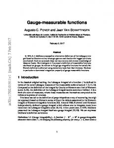
Figure 2: The Young diagram for the partition k “ p8, 7, 7, 5, 4, 3, 3, 2, 2, 1q of |k| “ 42 with quantities defined in the text and the relationship between the two different conventions: English (panel (a) and Russian (panel (b) ).

where for a given k P N0 |ks pkq| ” k “

N ÿ

α“1

nα “

N ÿ

α“1

|ksα pnα q| “

ℓα N ÿ ÿ

α“1 iα “1

kisαα pnα q.

(A.20)

for any sα P t1, . . . , ppnα qu with α “ 1, . . . , N . Note that any ks pkq is uniquely specified by the ś set of numbers sα and nα , such that for a fixed nα for all α we have ppnα q number of different ks pkq’s. The above equation represents a specific decomposition of k into a sum of parts nα . However, this decomposition is not unique. In fact, there is a cpn, N q “ pn ` N ´ 1q!{pN ´ 1q!n! possible ways to do this, where cpn, N q is a number of constrained partitions (so called compositions) of n P N0 into a sum of exactly N parts. Let Spk, N q denote a shell in YN , that ˇ ( is a set of points defined as follows Spk, N q ” k P YN ˇ|k| “ k , then the number of points in the shell amounts to cpk,N N ÿqź ppnrα q. #Spk, N q “ r“1 α“1

This enables us to decompose the sum in the instanton part of Eq. (4.1b) into a sum over distinct shells and the sum over points in a given shell, namely ÿ

kPYN

Λ2N |k| Zk pa, ǫ1 , ǫ2 q “

ÿ

Λ2N k

kě0

ÿ

kPSpk,N q

Zk pa, ǫ1 , ǫ2 q.

(A.21)

Sum over shells amounts to ÿ

kPSpk,N q

Zk pa, ǫ1 , ǫ2 q “

r cpk,N N ppn ÿqź ÿα q

r“1 α“1 sα “1

Zinst pa, tksα pnrα qu, ǫ1 , ǫ2 q.

(A.22)

Instead of regarding sth partition ks pnq as a ℓ-tuple of non-increasing, positive integers one can extend this notion to an infinite sequence of non-increasing, nonnegative integers ki whose length is ℓpkq “ ℓ, and for i ą ℓ, ki “ 0. Moreover, we follow the practice to keep implicit both,

35

the label s that positions a partition in Pn and the number n the relevant partition corresponds to. Within this extended notion, the partition is the following sequence ÿ k “ tki uiPN , where ki P N0 , i ą j ñ ki ď kj , |k| “ ki “ n.

@

i,jPN

iě1

Note that this implies that for i Ñ 8, ki Ñ 0. Form this point of view, Y is a subset of nonnegative, integer null sequences c0 pZě0 q. For any partition (Young diagram) k P Y there ˜ P YD . It is related to the original one through the transposition, i.e., is a dual partition k ˜ “ kT (k ˜T “ k) and |k| ˜ “ |k|. Hence, Y – YD “ ReversepYq, where the last map is a specific k permutation that reverses the ordering o partitions within each Pn . Extension to a colored partition is straightforward and for any k P YN it takes the following form k “ pk1 , . . . , kN q “ tkα,i uαPt1,..,N u iPN

and k “ |k| “

N ÿ

α“1

|kα | “

N ÿ ÿ

kα,i .

α“1 iě1

Notions of partition theory play the crucial role in counting of instanton configurations. As it has been shown by Nekrasov [20] and independently by Nakajima and Yoshioka [56] the instanton part of the partition function for the N “ 2 nonabelian gauge theory with SU pN q symmetry, when computed on the so called Ω-background [19], appears to be a sum over all colored Young diagrams. The instanton charge k corresponds to the total number of boxes that are distributed into N parts (compositions) each of which can be further partitioned, thus forming a colored Young diagram as described above. The form of Nekrasov’s instanton partition function for a pure SU pN q gauge theory reads [19] ÿ ˆ a, ǫ1 , ǫ2 q “ ˆ 2N k Zk pa, ǫ1 , ǫ2 q, Zinst pΛ, Λ (A.23) kPYN

where

Zk pa, ǫ1 , ǫ2 q “

N ź ź

α,β“1 i,jě1

aα ´ aβ ` ǫ1 pi ´ 1q ` ǫ2 p´jq , aα ´ aβ ` ǫ1 pi ´ k˜β,j ´ 1q ` ǫ2 pkα,i ´ jq

(A.24a)

ˆ is an infrared effective scale which is related to the complexified SU pN q gauge couwhere Λ ˆ 2N „ µ2N expt2πiτ u. µU V is the scale where the classical pling τ “ 4πi{g2 ` θ{2π through Λ UV (microscopic) theory is defined. The deformation parameters are in general ǫ1,2 P C and either ℜpǫ1 q ą 0, ℜpǫ2 q ă 0 or ℜpǫ1 q ă 0, ℜpǫ2 q ą 0. For the sake of definiteness in what follows we assume ℜpǫ1 q ą 0, ℜpǫ2 q ă 0. The contribution (A.24a) to eq. (A.23) may be cast into three equivalent forms, which we quote following ref. [19], namely Zk pa, ǫ1 , ǫ2 q “

N ź ź

aαβ ` ǫ1 p´iq ` ǫ2 pj ´ 1q ` ǫ1 pk˜α,j ´ iq ` ǫ2 pj ´ kβ,i ´ 1q

aαβ ź Γ pbαβ ` νpj ´ i ` 1q ` kαi ´ kβj q Γ pbαβ ` νpj ´ iqq Γ pbαβ ` νpj ´ iq ` kαi ´ kβj q Γ pbαβ ` νpj ´ i ` 1qq

α,β“1 i,jě1

“

1 k ǫ2N 2

“

N ź

(A.24b) (A.24c)

pα,iq‰pβ,jq

ź

α,β“1 sPkα

aαβ

ź 1 1 ` ˘ ` ˘ , ´ ǫ1 Lβ psq ` ǫ2 Aα psq ` 1 sPk aαβ ` ǫ1 Lα psq ` 1 ´ ǫ2 Aβ psq β

36

(A.24d)

where aαβ ” aα ´ aβ ,

bαβ ” aαβ {ǫ2 ,

ν ” ´ǫ1 {ǫ2 ,

and Aα psq ” kα,i ´ j, Lα psq ” k˜α,j ´ i are arm-length and leg-length, respectively. s ” pi, jq represents a box in a Young diagram kα , where 1 ď i ď ℓα “ k˜α,1 and 1 ď j ď kα,i . The forms (A.24a) – (A.24c) although defined in terms of infinite product are finite and well defined due to a finiteness of the relevant Young diagrams. In what follows we are concerned with yet another form, namely the contribution expressed in terms of the profiles of Young diagrams. This form can be obtained by means of the ζ-function regularization techniques that enable to deal with divergent expressions like the numerator or the denominator of eq. (A.24a) when considered separately. The contribution (A.24a) to the instanton partition function (A.23) along with the perturbative part introduced in eq. (4.1a) can be cast into the following form $ , N & ÿ . Λ2N k exp ´ γǫ1 ,ǫ2 paαβ ; Λq Zk pa, ǫ1 , ǫ2 q % α,β“1 $ 8 & d ˇˇ s ż 1 Λ dt ts´1 ǫ1 t “ exp ´ ˇˇ % ds s“0 Γpsq pe ´ 1qpeǫ2 t ´ 1q 0 ff, « N ¯ . ÿ ÿ ´ ˜ eaαβ t ` pe´ǫ1 t ´ 1qpeǫ2 t ´ 1q etraαβ `ǫ1 pi´kβj q`ǫ2 pkαi ´jqs ´ etraαβ `ǫ1 i´ǫ2 js , ˆ i,jě1 α,β“1

(A.25)

where the perturbative part is defined in eq. (4.1a) with the ǫ1 ǫ2 -parametric gamma function assumes a form (recall that we take ℜǫ1 ą 0, ℜǫ2 ă 0) 8 ˇ ˆs ż ˇ d Λ e´xt s´1 ˆ ” ˇ γǫ1 ,ǫ2 px; Λq , dt t ds ˇs“0 Γpsq peǫ1 t ´ 1qpeǫ2 t ´ 1q

ℜx ą 0, ℜs ą 2.

(A.26)

0

The above gamma function satisfies the following second order functional partial difference equation ¸ ˜ ˆ Λ ˆ “ log , ∆ǫ1 ∆ǫ2 γǫ1 ,ǫ2 px; Λq x ` ǫ1 ` ǫ2 where ∆ǫi f pxq ” f px ` ǫi q ´ f pxq for i “ 1, 2. For convenience we introduce the following notation eα ptq ” eaα t , pptq ” e´ǫ1 t , qptq ” eǫ2 t , ℜpǫ1 q ą 0, ℜpǫ2 q ă 0. (A.27) With this notation the formula in the last line of eq. (A.25) reads ˇ ż8 Λs d ˇˇ 1 ´ ˇ dt ts´1 ´1 ds s“0 Γpsq pp ´ 1qpq ´ 1q 0 + # N ¯ ÿ ÿ ´ ˜ ´1 kβj ´i kαi ´j ´i ´j ˆ , (A.28) eα eβ 1 ` pp ´ 1qpq ´ 1q p q ´p q i,jě1

α,β“1

37

The above series can be transformed into the finite form, namely (ℓ˜α “ ℓpkTα q “ kα,1 ) 1 ` pp ´ 1qpq ´ 1q

¯ ÿ ´ ˜ pkβj ´i q kαi ´j ´ p´i q ´j

i,jě1

˜

“1 ` pp ´ 1qpq ´ 1q ` pp ´ 1q «

ℓα ÿ

p

´i

i“1 j“1

´ ¯´ ¯ ˜ p´i q ´j pkβj ´ 1 q kαi ´ 1

ℓ˜β ´ ¯ ´ ¯ ÿ ˜ kαi q ´j pkαj ´ 1 q ´ 1 ` pq ´ 1q

(A.29)

j“1

i“1

“ 1 ` pp ´ 1q

ℓβ ℓα ÿ ÿ

ℓα ÿ

fi ff» ℓ˜β ¯ ´ ¯ ÿ ˜ ´ 1 –1 ` pq ´ 1q q ´j pkβj ´ 1 fl .

´

p´i q kαi

i“1

j“1

In what follows it proves useful to define the following quantity ϕkα pp, qq ” 1 ` pp ´ 1q

ℓα ÿ

i“1

´ ¯ p´i q kαi ´ 1 .

(A.30)

Note, that in the above formula we can extend the upper sum limit ℓα up to infinity which leaves its form intact. Multiplying eq. (A.30) by eα , summing over color index and rewriting it back in the original form as in eq. (A.27) we obtain N ÿ

α“1

eα ϕkα pp, qq “

N ÿ

α“1

eaα t `

N ÿ´ ÿ

α“1 iě1

¯ eraα `ǫ1 pi´1q`ǫ2 kαi st ´ eraα `ǫ1 i`ǫ2 kαi st ´ eraα `ǫ1 pi´1qst ` eraα `ǫ1 ist .

which can be written as 1 2

ż

dx

2 fa,k px|ǫ1 , ǫ2 qext

“

R

N ÿ

α“1

` ˘ eα ptqϕkα pptq, qptq ,

(A.31a)

where fa,k px|ǫ1 , ǫ2 q “

N ÿ

α“1

|x ´ aα | `

N ÿ´ ÿ

α“1 iě1

|x ´ xα,i | ´ |x ´ xα,i ´ ǫ1 |

ˇ ˇ ˇ ˇ¯ ´ ˇx ´ x0α,i ˇ ` ˇx ´ x0α,i ´ ǫ1 ˇ , (A.31b)

is the profile function of the colored Young diagram kα . In analogy to the above, one defines for the second factor of the last line of eq. (A.29) the following form of the profile 1 2

ż

dx

2 ´xt fa,k T px|ǫ2 , ǫ1 qe

“

R

38

N ÿ

α“1

pqptq, pptqq, e´1 α ptqϕkT α

(A.31c)

and fa,kT px|ǫ2 , ǫ1 q “

N ÿ

α“1

|x ` aα | `

N ÿ´ ÿ

α“1 iě1

|x ´ x ˜α,i | ´ |x ´ x ˜α,i ´ ǫ2 |

ˇ ˇ ˇ ˇ¯ ´ ˇx ´ x ˜0α,i ˇ ` ˇx ´ x ˜0α,i ´ ǫ2 ˇ . (A.31d)

This form of the profile function equals to the one in eq. (A.31b) as it takes its form from subjecting the former to the transposition of the Young diagram and subsequent reversion of the order of pair of parameters pǫ1 , ǫ2 q Ñ pǫ2 , ǫ1 q . It stems from the fact that in case of the arbitrary Young diagram the following identity holds true ÿ

pi,jqPk

`

i j

pq “

ki ℓ ÿ ÿ

i“1 j“1

˜

i j

pq “

kj ℓ˜ ÿ ÿ

j“1 i“1

pi q j “

ÿ

pi q j .

(A.32)

pj,iqPkT

˘ It entails that ϕkα pptq, qptq “ ϕkTα pqptq, pptqq and from eq. (A.27) it results that p´1 ptq “ pp´tq which holds true also for q and eα . Hence, we obtain the equality fa,k px|ǫ1 , ǫ2 q “ fa,kT px|ǫ2 , ǫ1 q. Using the two expressions for the profile functions we obtain the exponent of right hand side of faα ,kα px|~, ´~q

xα,1 xα,2

aα

xα,ℓα

x

Figure 3: This is the profile function (thick line) for the colored Young diagram of fig. 2 with the columns projected onto R axis.

eq. (A.25) in the sought form, namely ˇ ż8 N ÿ d ˇˇ 1 Λs ´ ˇ dt ts´1 ´1 pq, pq eα e´1 β ϕkα pp, qqϕkT β ds s“0 Γpsq pp ´ 1qpq ´ 1q α,β“1 0 ij 1 2 2 px|ǫ1 , ǫ2 qγǫ1 ,ǫ2 px ´ y; Λqfa,k (A.33) “ ´ ´´ dxdy fa,k T py|ǫ2 , ǫ1 q. 4 R2

The partition function for the N “ 2 pure gauge theory with SU pN q symmetry takes now the form $ , & 1ij . ÿ 2 2 ZpΛ, a, ǫ1 , ǫ2 q “ exp ´ ´´ dxdy fa,k px|ǫ1 , ǫ2 qγǫ1 ,ǫ2 px ´ y; Λqfa,k , (A.34) T py|ǫ2 , ǫ1 q % 4 f PF a,k

R2

39

Due to the fact that the profile function equals its (parameter) reverse (Young diagram) transpose, the exponent in the above formula can be cast into yet two equivalent forms with exponents ˆ 2 qj pǫ1 , ǫ2 q. The ˆ 2 qj pǫ1 , ǫ2 q and pf 2 qi pǫ1 , ǫ2 qγij pΛqpf that have schematic form pfk2T qi pǫ2 , ǫ1 qγij pΛqpf k k k last two correspond to eqs. (A.24b) and (A.24c), respectively multiplied by the perturbative part. This statement can be phrased yet in another form. Let us define the following quantity Nαβ pp, qq ”

ϕkα pp, qqϕkT pq, pq ´ 1 β

pp´1 ´ 1qpq ´ 1q

(A.35)

.

Then the left hand side of eq. (A.33) can be put in the form ij 1 2 2 px|ǫ1 , ǫ2 qγǫ1 ,ǫ2 px ´ y; Λqfa,k ´ ´´ dxdy fa,k T py|ǫ2 , ǫ1 q 4 R2

8 ˇ N ÿ ˆs ż ˇ Λ d s´1 ˇ ˆ “´ dt t γǫ1 ,ǫ2 paαβ ; Λq ´ ˇ eα e´1 β Nαβ pp, qq. ds Γpsq s“0 α,β“1 α,β“1 N ÿ

0

The quantity under the second integral with the use of eq. (A.32) can be brought to the following equivalent forms N ÿ

α,β“1

eα e´1 β Nαβ pp, qq

“´ “´

N ÿ

eα e´1 β eα e´1 β

α,β“1

(A.36a)

i,jě1

α,β“1 N ÿ

¯ ÿ ´ ˜ pkβj ´i`1 q kαi ´j ´ p´i`1 q ´j

¯ ÿ ´ ˜ p´kαj `i q ´kβi `j´1 ´ pi q j´1

(A.36b)

i,jě1

¯ p ´ 1 ´ kαi ´kβj j´i (A.36c) q p ´ pj´i q´1 pα,iq‰pβ,jq ˛ ¨ N ÿ ÿ ÿ ˝ p´Lα psq q ´Aβ psq´1 ‚. (A.36d) pLβ psq`1 q Aα psq ` “´ eα e´1 β ÿ

“

eα e´1 β

α,β“1

sPkβ

sPkα

The ordering of the above equations corresponds to the one in eqs. (A.24a) – (A.24d). The definition of Aα and Lα can be found below the latter equation. The ”off-diagonal” sum in eq. (A.36c) is understood as follows ÿ

pα,iq‰pβ,jq

A.5

Aα,i;β,j “

N ÿ ÿ

α“1 i‰j

Aα,i;α,j `

N ÿ ÿ

Aα,i;β,j .

α‰β i,j

Product identities and Y functions

The saddle point equation can be given yet another form. First, let us note that the following identities hold L N ź N ź ź x ´ x0α,j ` ǫ1 x ´ x0α,1 ` ǫ1 . (A.37a) “ x ´ x0α,j x ´ x0α,1 ´ ǫ1 pL ´ 1q α“1 j“1 α“1 40

Shifting the above equation in x Ñ x ´ ǫ1 and multiplying thus obtained result by the eq. (A.37a) leads to the following identity N ź L 2 ź x ´ x0α,j ` ǫ1 ź

α“1 j“1

x ´ x0α,j

N ź 2 ź ǫ1 ǫ1 “ . ´ ǫ1 j“1 x ´ x0α,j ` ǫ1 α“1 j“1 x ´ x0α,j ´ ǫ1 pL ´ 1q

(A.37b)

As the first step to the iterative solution of eq. (4.21) one assumes that there exists some L P N at which a sequence of columns terminates, i.e., ωα,i “ 0 for i ą L. In this case the only change in the saddle point equation (4.21) is 2 N ź px 0 ź α,i ´ xβ,j ´ ǫ1 qpxα,i ´ xβ,j ` ǫ1 q ź

β“1 jě1

pxα,i ´ xβ,j ` ǫ1 qpxα,i ´ “

x0β,j

ǫ1 ´ ǫ1 q j“1 xα,i ´ x0β,j ` ǫ1

N ź 2 L px 0 ź α,i ´ xβ,j ´ ǫ1 qpxα,i ´ xβ,j ` ǫ1 q ź

ǫ1 0 ´ǫ q 0 `ǫ . px ´ x ` ǫ qpx ´ x x ´ x α,i 1 α,i 1 α,i 1 β,j β,j β,j j“1 β“1 j“1

Due to identity in eq. (A.37b) it is possible to rewrite the right hand side of the above equation in the form 2 N ź N ź L ź ź xα,i ´ xβ,j ´ ǫ1 xα,i ´ xβ,j ´ ǫ1 ź ǫ1 2N . “ ǫ 1 0 x ´ x ` ǫ x ´ x ` ǫ x ´ x ´ ǫ pL ´ 1q α,i 1 α,i 1 β,j β,j α,i 1 β,j j“1 β“1 jě1 β“1 j“1

Hence, the saddle point equation takes the infinite product form (ξα,i ” xα,i {ǫ1 ) ˆ 2N Λ

N ź N ź ź ź xα,i ´ xβ,j ´ ǫ1 ξα,i ´ ξβ,j ´ 1 ˆ 1 q2N “ p´1qN ´1 , “ pΛ{ǫ x ´ x ` ǫ ξ ´ ξ ` 1 α,i 1 α,i β,j β,j β“1 jě1 β“1 jě1

(A.38)

It is now possible to release the condition for the finiteness of the number of columns such that tω i uL i“1 Ñ tω i uiPN , which leave the form of the equation intact. As one may notice, this form resembles TBA equation. Before we proceed, let us rewrite the saddle point equation using the following function U pzq ”

N ź ź z{ǫ1 ´ 1 ´ ξβ,j , z{ǫ ` 1 ´ ξ 1 β,j β“1 jě1

ˆ 1 q2N U pxα,i q “ p´1qN ´1 . pΛ{ǫ

Note, that numerator and denominator if taken separately are divergent. For the study of noniterative solution of eq. (A.38) it is convenient to work with well defined functions. Therefore, following Poghossian [53] we bring the saddle point equation into yet another form. Namely, let us cast U pzq function back into the form of eq. (4.21) with the cutoff L for safety reasons, i.e., N ź L pz ´ x 0 ź ǫ2N β,j ´ ǫ1 qpz ´ xβ,j ` ǫ1 q 1 UL pzq “ P pzqP pz ` ǫ1 q β“1 j“1 pz ´ xβ,j ` ǫ1 qpz ´ x0β,j ´ ǫ1 q

´ N L 2N ź ź 1´ ǫ1 “ P pzqP pz ` ǫ1 q β“1 j“1 ´ 1´ 41

z´ǫ1 xβ,j z`ǫ1 xβ,j

¯ˆ ¯ˆ

1´

z`ǫ1 x0β,j

1´

z´ǫ1 x0β,j

˙

˙ , (A.39)

where P pzq ” N ź L ˆ ź

β“1 j“1

ś

1´

pz ´ aα q. Each factor of the above product may be transformed as follows z

xβ,j

˙

z{x0β,j ´z{x0β,j

e

e

“

N ź

e

β“1

j“1

˜

´ ǫz N γ` 1

“e where ψL pz ` 1q ” ´γ `

L ˆ ÿ 1

i

i“1

L ř

´pz{ǫ1 q

L ř

j“1

1 j

L ˆ pǫ1 {x0β,j q ź

¸

j“1

N ź

e

1´

z xβ,j

pz{ǫ1 qψL paβ {ǫ1 q

1 z`i

˙

0

ez{xβ,j

L ˆ ź

j“1

β“1

´

˙

1´

z xβ,j

˙

0

ez{xβ,j ,

d log Γpz ` 1q. dz

LÑ8

ÝÝÝÑ ψpz ` 1q “

Inserting this result in the appropriate form into the eq. (A.39) we get ˆ ´ ¯ pz´ǫ1 q{x0β,j z´ǫ1 1 ´ e 1´ L N xβ,j ź ǫ2N e2pz{ǫ1 qψL paβ {ǫ1 q ź 1 ˆ UL pzq “ ¯ P pzqP pz ` ǫ1 q β“1 e2pz{ǫ1 qψL paβ {ǫ1 q j“1 ´ pz`ǫ1 q{x0β,j z`ǫ1 1´ 1 ´ xβ,j e

z`ǫ1 x0β,j z´ǫ1 x0β,j

˙ ˙

0

epz`ǫ1 q{xβ,j . e

pz´ǫ1 q{x0β,j

Each factor in the numerator and the denominator are now separately well defined. Within the limit L Ñ 8 these functions resemble inverse of the Gamma function which is known to be entire function. Define the following quantities Y pzq ” Y0 pzq ”

N ź

´pz{ǫ1 qψpaβ {ǫ1 q

e

jě1

β“1 N ź

źˆ

´pz{ǫ1 qψpaβ {ǫ1 q

e

ź

jě1

β“1

1´

˜

1´

z xβ,j z x0β,j

˙

¸

0

ez{xβ,j , (A.40) e

z{x0β,j

.

These are either entire functions with zeros at points xβ,j , x0β,j respectively. We can now safely send L Ñ 8 so that the result reads U pzq “

ǫ2N Y pz ´ ǫ1 qY0 pz ` ǫ1 q Y pz ´ ǫ1 q 1 “ . P pzqP pz ` ǫ1 q Y pz ` ǫ1 qY0 pz ´ ǫ1 q Y pz ` ǫ1 q

(A.41)

With the aid of these functions the saddle point equation (A.38) can now be expressed in yet another enlightening form given in eq. (4.26).

A.6

The result of iterative solution of the saddle point equation for SU(2)

In this appendix we present results of iterative solution of the saddle point equation (4.21). This is done up to L “ 3, where L is a cutoff for number of columns within each colored Young ˆ 1 q2N of colored column diagram. Quantities obtained this way are coefficients of expansion in pΛ{ǫ in an extreme Young diagram, namely ω˚ α,i “

ÿ

ωα,i,j qj ,

jěi

42

ˆ 1 q2N . q ” pΛ{ǫ

The sum over colors within a given order of q expansion yields coefficients of the twisted superpotential. The saddle potint equation given in eq. (4.21) which is to be soleved iteratively in this appendix may be rewritten in a more useful form, namely qǫ2N 1

L ´ N ź ź

pLq xα,i

α“1 j“1

`

´

x0β,j

2 ´ N ź ź

α“1 j“1

¯ ¯´ pLq pLq ` ǫ1 xα,i ´ xβ,j ´ ǫ1

pLq

xα,i ´ x0β,j ` ǫ1

L ´ ¯ź j“1

pLq

xα,i ´ x0β,j ´ ǫ1

¯ ¯´ pLq pLq xα,i ´ xβ,j ` ǫ1 “ 0. (A.42)

• N “ 2, L “ 1 ω1,1,1 “ ´

ǫ31 , 2ap2a ` ǫ1 q

ω2,1,1 “ ´

ǫ31 . 2a p2a ´ ǫ1 q

(A.43a)

• N “ 2, L “ 2

ω1,1,2 ω1,2,2 ω2,1,2 ω2,2,2

˘ ` ǫ51 ´8a5 ` 4a4 ǫ1 ` 22a3 ǫ21 ` 3a2 ǫ31 ` 3aǫ41 ` ǫ51 , “´ 8a3 p2a ´ ǫ1 q 2 pa ` ǫ1 q p2a ` ǫ1 q 3 ǫ51 “´ , 8a pa ` ǫ1 q p2a ` ǫ1 q 2 ˘ ` ǫ51 8a5 ` 4a4 ǫ1 ´ 22a3 ǫ21 ` 3a2 ǫ31 ´ 3aǫ41 ` ǫ51 “ 8a3 pa ´ ǫ1 q p2a ´ ǫ1 q 3 p2a ` ǫ1 q 2 ǫ51 “´ . 8a pa ´ ǫ1 q p2a ´ ǫ1 q 2

(A.43b) (A.43c) (A.43d) (A.43e)

• N “ 2, L “ 3 In this case the solutions are for α “ 1 ˘ ` ǫ71 896a12 ´ 1600a11 ǫ1 ´ 2656a10 ǫ21 ω1,1,3 “ ´ 96a5 pa ´ ǫ1 q 2 pǫ1 ´ 2aq 4 pa ` ǫ1 q p2a ` ǫ1 q 5 p2a ` 3ǫ1 q ˘ ` ǫ71 7344a9 ǫ31 ` 3000a8 ǫ41 ´ 7788a7 ǫ51 ` 7102a6 ǫ61 ´ 96a5 pa ´ ǫ1 q 2 pǫ1 ´ 2aq 4 pa ` ǫ1 q p2a ` ǫ1 q 5 p2a ` 3ǫ1 q ˘ ` 12 11 ǫ71 ´2999a5 ǫ71 ´ 677a4 ǫ81 ´ 144a3 ǫ91 ´ 96a2 ǫ10 1 ` 30aǫ1 ` 18ǫ1 , ´ 96a5 pa ´ ǫ1 q 2 pǫ1 ´ 2aq 4 pa ` ǫ1 q p2a ` ǫ1 q 5 p2a ` 3ǫ1 q ˘ ` 2ǫ71 ´2a3 ´ a2 ǫ1 ` 5aǫ21 ` ǫ31 ω1,2,3 “ ´ , 3a pǫ1 ´ 2aq 2 pa ` ǫ1 q p2a ` ǫ1 q 4 p2a ` 3ǫ1 q ǫ7 ` 1 ˘ , ω1,3,3 “ ´ 96a p2a ` 3ǫ1 q 2a2 ` 3aǫ1 ` ǫ21 2

43

(A.43f) (A.43g) (A.43h)

and for α “ 2 ω2,1,3

ω2,2,3

˘ ` ǫ71 896a12 ` 1600a11 ǫ1 ´ 2656a10 ǫ21 ` ˘ “´ 96a5 p2a ´ ǫ1 q 5 pa ` ǫ1 q 2 p2a ` ǫ1 q 4 2a2 ´ 5aǫ1 ` 3ǫ21 ˘ ` ǫ71 ´7344a9 ǫ31 ` 3000a8 ǫ41 ` 7788a7 ǫ51 ` 7102a6 ǫ61 ` ˘ ´ 96a5 p2a ´ ǫ1 q 5 pa ` ǫ1 q 2 p2a ` ǫ1 q 4 2a2 ´ 5aǫ1 ` 3ǫ21 ˘ ` 11 12 ǫ71 2999a5 ǫ71 ´ 677a4 ǫ81 ` 144a3 ǫ91 ´ 96a2 ǫ10 1 ´ 30aǫ1 ` 18ǫ1 ` ˘ , ´ 96a5 p2a ´ ǫ1 q 5 pa ` ǫ1 q 2 p2a ` ǫ1 q 4 2a2 ´ 5aǫ1 ` 3ǫ21 ˘ ` 2ǫ71 2a3 ´ a2 ǫ1 ´ 5aǫ21 ` ǫ31 ` ˘, “ 3a pǫ1 ´ 2aq 4 p2a ` ǫ1 q 2 2a2 ´ 5aǫ1 ` 3ǫ21

ω2,3,3 “ ´

References

ǫ7 ` 1 ˘ . 96a p2a ´ 3ǫ1 q 2a2 ´ 3aǫ1 ` ǫ21 2

(A.43i)

(A.43j) (A.43k)

[1] E. Mathieu, M´emoire sur le mouvement vibratoire d’une membrane de forme elliptique, Jour. de Math. Pures et Appliquees (Jour. de Liouville) 13 (1868) 137. [2] E. Whittaker and G. Watson, A course of modern analysis. Cambridge Mathematical Library. Cambridge University Press, 1996. [3] N. W. McLachlan, Theory and application of Mathieu functions. Oxford : Clarendon Press, 1947. [4] H. M¨ uller-Kirsten, Introduction to Quantum Mechanics: Schr¨ odinger Equation and Path Integral. World Scientific, 2006. [5] W. Paul, Electromagnetic traps for charged and neutral particles, Rev.Mod.Phys. 62 (1990) 531–540. [6] S. S. Gubser and A. Hashimoto, Exact absorption probabilities for the D3-brane, Commun.Math.Phys. 203 (1999) 325–340, [hep-th/9805140]. [7] R. Manvelyan, H. Muller-Kirsten, J. Liang, and Y. bo Zhang, Absorption cross-section of scalar field in supergravity background, Nucl.Phys. B579 (2000) 177–208, [hep-th/0001179]. [8] D. Park, S. Tamarian, H. Muller-Kirsten, and J. zu Zhang, D-branes and their absorptivity in Born-Infeld theory, Nucl.Phys. B594 (2001) 243–271, [hep-th/0005165]. [9] J. Lachapelle, A study of the growth of entropy fluctuations during reheating in Roulette inflation. Master Thesis, McGill University, 2008. [10] Y. Cho, N. Kan, and K. Shiraishi, Compactification in deconstructed gauge theory with topologically nontrivial link fields, Acta Phys.Polon. B35 (2004) 1597–1606, [hep-th/0306012]. 44

[11] M. Reed and B. Simon, Methods of modern mathematical physics, Vol 4., Analysis of operators. [12] A. Gorsky, I. Krichever, A. Marshakov, A. Mironov, and A. Morozov, Integrability and Seiberg-Witten exact solution, Phys.Lett. B355 (1995) 466–474, [hep-th/9505035]. [13] N. Seiberg and E. Witten, Electric - magnetic duality, monopole condensation, and confinement in N=2 supersymmetric Yang-Mills theory, Nucl.Phys. B426 (1994) 19–52, [hep-th/9407087]. [14] A. Mironov and A. Morozov, Nekrasov Functions and Exact Bohr-Zommerfeld Integrals, JHEP 1004 (2010) 040, [arXiv:0910.5670]. [15] W. He, Sine-Gordon quantum mechanics on the complex plane and N=2 gauge theory, Phys.Rev. D81 (2010) 105017. [16] K. Maruyoshi and M. Taki, Deformed Prepotential, Quantum Integrable System and Liouville Field Theory, Nucl. Phys. B841 (2010) 388–425, [arXiv:1006.4505]. [17] N. A. Nekrasov and S. L. Shatashvili, Quantization of Integrable Systems and Four Dimensional Gauge Theories, 2009. [18] A. Mironov and A. Morozov, Nekrasov Functions from Exact BS Periods: The Case of SU(N), J.Phys. A43 (2010) 195401, [arXiv:0911.2396]. [19] N. Nekrasov and A. Okounkov, Seiberg-Witten Theory and Random Partitions, hep-th/0306238v2. [20] N. A. Nekrasov, Seiberg-Witten prepotential from instanton counting, Adv.Theor.Math.Phys. 7 (2004) 831–864. [21] N. A. Nekrasov and S. L. Shatashvili, Supersymmetric vacua and Bethe ansatz, Nucl.Phys.Proc.Suppl. 192-193 (2009) 91–112, [arXiv:0901.4744]. [22] N. A. Nekrasov and S. L. Shatashvili, Quantum integrability and supersymmetric vacua, Prog.Theor.Phys.Suppl. 177 (2009) 105–119, [arXiv:0901.4748]. [23] N. Nekrasov, V. Pestun, and S. Shatashvili, Quantum geometry and quiver gauge theories, arXiv:1312.6689. [24] L. F. Alday, D. Gaiotto, and Y. Tachikawa, Liouville Correlation Functions from Four-dimensional Gauge Theories, Lett.Math.Phys. 91 (2010) 167–197, [arXiv:0906.3219]. [25] N. Wyllard, AN ´1 conformal Toda field theory correlation functions from conformal N = 2 SU(N) quiver gauge theories, JHEP 0911 (2009) 002, [arXiv:0907.2189].

45

[26] J. Teschner, Quantization of the Hitchin moduli spaces, Liouville theory, and the geometric Langlands correspondence, [hep-th/1005.2846]. [27] D. Gaiotto, Asymptotically free N=2 theories and irregular conformal blocks, arXiv:0908.0307. [28] J. Hempel, On the uniformization of the n-punctured sphere, Bull. London Math. Soc. 20 (1988) 97. [29] L. Keen, H. Rauch, and A. Vasquez, Moduli of punctured tori and the accessory parameter of Lam´e’s equation, Trans. Am. Math. Soc. 255 (1979) 201. [30] A. B. Zamolodchikov and A. B. Zamolodchikov, Structure constants and conformal bootstrap in Liouville field theory, Nucl.Phys. B477 (1996) 577–605, [hep-th/9506136]. [31] L. Hadasz and Z. Jaskolski, Liouville theory and uniformization of four-punctured sphere, J.Math.Phys. 47 (2006) 082304, [hep-th/0604187]. [32] P. Menotti, On the monodromy problem for the four-punctured sphere, arXiv:1401.2409. [33] P. Menotti, Hyperbolic deformation of the strip-equation and the accessory parameters for the torus, JHEP 1309 (2013) 132, [arXiv:1307.0306]. [34] P. Menotti, Accessory parameters for Liouville theory on the torus, JHEP 1212 (2012) 001, [arXiv:1207.6884]. [35] P. Menotti, Riemann-Hilbert treatment of Liouville theory on the torus: The general case, J.Phys. A44 (2011) 335401, [arXiv:1104.3210]. [36] P. Menotti, Riemann-Hilbert treatment of Liouville theory on the torus, J.Phys. A44 (2011) 115403, [arXiv:1010.4946]. [37] M. Piatek, Classical torus conformal block, N “ 2˚ twisted superpotential and the accessory parameter of Lame equation, JHEP 1403 (2014) 124, [arXiv:1309.7672]. [38] F. Ferrari and M. Piatek, Liouville theory, N=2 gauge theories and accessory parameters, JHEP 1205 (2012) 025, [arXiv:1202.2149]. [39] V. V. Bazhanov and S. L. Lukyanov, Integrable structure of Quantum Field Theory: Classical flat connections versus quantum stationary states, arXiv:1310.4390. [40] A. Litvinov, S. Lukyanov, N. Nekrasov, and A. Zamolodchikov, Classical Conformal Blocks and Painleve VI, arXiv:1309.4700. [41] T. Hartman, Entanglement Entropy at Large Central Charge, arXiv:1303.6955. [42] A.-K. Kashani-Poor and J. Troost, The toroidal block and the genus expansion, JHEP 1303 (2013) 133, [arXiv:1212.0722]. 46

[43] A. Marshakov, A. Mironov, and A. Morozov, On non-conformal limit of the AGT relations, Phys. Lett. B682 (2009) 125–129, [arXiv:0909.2052]. [44] L. Hadasz, Z. Jaskolski, and P. Suchanek, Proving the AGT relation for Nf “ 0, 1, 2 antifundamentals, JHEP 1006 (2010) 046, [arXiv:1004.1841]. [45] D. Maulik and A. Okounkov, Quantum Groups and Quantum Cohomology, arXiv:1211.1287. [46] V. Alba and A. Morozov, Non-conformal limit of AGT relation from the 1-point torus conformal block, JETP Lett. 90 (2009) 708–712, [arXiv:0911.0363]. [47] A. Zamolodchikov, Conformal symmetry in two-dimensional space: recursion representation of conformal block, Theor. Math. Phys. 73 (1987) 1088. [48] A. Zamolodchikov, Two-dimensional conformal symmetry and critical four-spin correlation functions in the Ashkin-Teller model, Sov. Phys. JEPT 63 (1986) 1061. [49] G. W. Moore and N. Seiberg, Classical and Quantum Conformal Field Theory, Commun. Math. Phys. 123 (1989) 177. [50] A. Belavin, A. M. Polyakov, and A. Zamolodchikov, Infinite Conformal Symmetry in Two-Dimensional Quantum Field Theory, Nucl. Phys. B241 (1984) 333–380. [51] B. Feigin and D. Fuchs, Representations of the Virasoro algebra, Adv. Stud. Contemp. Math. 7 [Representation of Lie groups and related topics] (1990) 465–554. [52] J. Teschner, Liouville theory revisited, Class. Quant. Grav. 18 (2001) R153–R222, [hep-th/0104158]. [53] R. Poghossian, Deforming SW curve, JHEP 1104 (2011) 033, [arXiv:1006.4822]. [54] E. Perlmutter, Comments on Renyi entropy in AdS3 /CFT2 , JHEP 1405 (2014) 052, [arXiv:1312.5740]. [55] V. Fateev and A. Litvinov, On AGT conjecture, JHEP 1002 (2010) 014, [arXiv:0912.0504]. [56] H. Nakajima and K. Yoshioka, Instanton counting on blowup. I. 4-dimensional pure gauge theory, Inventiones Mathematicae 162 (June, 2005) 313–355, [math/0306198].

47