Feb 19, 2015 - Ritabrata Dutta and Samuel Kaski .... analysis (LDA) yields a discriminability of almost 100% (Figure 1(b), green dashed curve). If the data are ...
arXiv:1502.05503v1 [stat.CO] 19 Feb 2015
Classification and Bayesian Optimization for Likelihood-Free Inference Michael U. Gutmann and Jukka Corander Dept of Mathematics and Statistics University of Helsinki and HIIT, Finland {michael.gutmann, jukka.corander}@helsinki.fi Ritabrata Dutta and Samuel Kaski Dept of Information and Computer Science Aalto University and HIIT, Finland {ritabrata.dutta, samuel.kaski}@aalto.fi
Abstract Some statistical models are specified via a data generating process for which the likelihood function cannot be computed in closed form. Standard likelihood-based inference is then not feasible but the model parameters can be inferred by finding the values which yield simulated data that resemble the observed data. This approach faces at least two major difficulties: The first difficulty is the choice of the discrepancy measure which is used to judge whether the simulated data resemble the observed data. The second difficulty is the computationally efficient identification of regions in the parameter space where the discrepancy is low. We give here an introduction to our recent work where we tackle the two difficulties through classification and Bayesian optimization.
1
Introduction
The likelihood function plays a central role in statistics and machine learning. It is the joint probability of the observed data X seen as a function of the model parameters of interest θ. We may assume that the data X are a realization of a two stage sampling process, Z ∼ p1 (Z|θ o ),
X ∼ p2 (X|Z, θ o ),
(1)
where Z are unobserved variables and θo are some fixed but unknown values of the model parameters. The likelihood function L(θ) is implicitly defined via an integral, Z L(θ) = p(X|θ) = p2 (X|Z, θ)p1 (Z|θ)dZ. (2) For many realistic data generating processes, the integral cannot be computed analytically in closed form, and numerical approximation is computationally too costly as well. Standard likelihood-based inference is then not feasible. But inference can be performed by using the possibility to simulate data from the model. Such simulation-based likelihoodfree inference methods have emerged in multiple disciplines: “Indirect inference” originated in economics (Gouriéroux et al., 1993), “approximate Bayesian computation” (ABC) in genetics (Beaumont et al., 2002; Marjoram et al., 2003; Sisson et al., 2007), or the “synthetic likelihood” approach in ecology (Wood, 2010). The different methods share the basic idea to identify the model parameters by finding values which yield simulated data that resemble 1
1
Result: N samples θ1 . . . θN for i = 1 to N do repeat Propose parameter θ Generate pseudo observed data Yθ ∼ p(Yθ |θ) until X ≈ Yθ
2 3 4 5 6 7
affects the speed of the inference affects the quality of the inference
set θ i = θ end Algorithm 1: Basic ABC algorithm.
the observed data. The inference process is shown in a schematic way in Algorithm 1 in the framework of ABC. In Algorithm 1, two fundamental difficulties of the aforementioned inference methods are highlighted. One difficulty is the measurement of similarity, or discrepancy, between the observed data X and the simulated data Yθ (line 5). The choice of discrepancy measure affects the statistical quality of the inference process. The second difficulty is of computational nature. Since simulating data Yθ can be computationally very costly, one would like to identify the region in the parameter space where the simulated data resemble the observed data as quickly as possible, without proposing parameters θ which have a negligible chance to be accepted (line 3). We have been working on both problems, the choice of the discrepancy measure and the fast identification of the parameter regions of interest (Gutmann et al., 2014; Gutmann and Corander, 2015). The following two sections are a brief introduction to the two papers.
2
Discriminability as discrepancy measure
We transformed the original problem of measuring the discrepancy between Yθ and X into a problem of classifying the data into simulated versus observed (Gutmann et al., 2014). Intuitively, it is easier to discriminate between two data sets which are very different than between data which are similar, and when the two data sets are generated with the same parameter values, the classification task cannot be solved significantly above chance-level. This motivated us to use the discriminability (classifiability) as discrepancy measure, and to perform likelihood-free inference by identifying the parameter values which yield chancelevel discriminability only (Gutmann et al., 2014). We next illustrate this approach using a toy example. The data X = (x1 , . . . , xn ) are assumed to be sampled from a standard normal distribution (black curve in Figure 1(a)), and the parameter of interest θ is the mean. For data simulated with mean θ = 6 (green curve), the two densities barely overlap so that classification is easy. In fact, linear discriminant analysis (LDA) yields a discriminability of almost 100% (Figure 1(b), green dashed curve). If the data are simulated with a mean closer to zero, for example with θ = 1/2 (red curve), the simulated data Yθ become more similar to X and the classification accuracy drops to around 60% (red dashed curve). For θ = 0, where the simulated and observed data are generated with the same values of θ, only chance-level discriminability of 50% is obtained. This illustrates how discriminability can be used as a discrepancy measure. We analyzed the validity of this approach theoretically and demonstrated it on more challenging synthetic data as well as real data with an individual-based epidemic model for bacterial infections in day care centers (Gutmann et al., 2014). The finding that classification can be used to measure the discrepancy has both practical and theoretical value: The main practical value is that the rather difficult problem of choosing a discrepancy measure is reduced to a more standard problem where we can leverage on effective existing solutions. The theoretical value lies in the establishment of a tight connection between likelihood-free inference and classification – two fields of research which appear rather different at first glance. 2
1
0.4
0.95 0.35
0.9 0.3
discriminability
0.85
pdf p(u)
0.25 0.2 0.15
0.8 0.75 0.7 0.65
0.1
0.6 0.05 0 -4
0.55 -2
0
2
4
6
8
0.5 -4
10
u
(a) Gaussian densities
-3
-2
-1
0
1
2
3 4 mean
5
6
7
8
9
(b) Classification performance of LDA
Figure 1: Discriminability as discrepancy measure, illustration on toy data (n = 10,000).
3
Bayesian optimization to identify parameter regions of interest
In the following, we denote a certain discrepancy measure by ∆θ . A small value of ∆θ is assumed to imply that Yθ are judged to be similar to X. The difficulty in finding parameter regions where ∆θ is small is at least twofold: First, the mapping from θ to ∆θ can generally not be expressed in closed form and derivatives are not available either. Second, ∆θ is actually a stochastic process due to the use of simulations to obtain Yθ . We illustrate this in Figure 2 for our Gaussian toy example where ∆θ is the discriminability between X and Yθ (for further examples, see Gutmann and Corander, 2015). The figure visualizes the distribution of ∆θ for n = 50. The fact that ∆θ is a random process was suppressed in Figure 1 by working with a large sample size. We used Bayesian optimization, a combination of nonlinear (Gaussian process) regression and optimization (see, for example, Brochu et al., 2010), to quickly identify regions where ∆θ is likely to be small (Gutmann and Corander, 2015). In Bayesian optimization, the (k) available information {(θ(k) , ∆θ ), k = 1, . . . , K} about the relation between θ and ∆θ is used to build a statistical model of ∆θ , and new data are actively acquired in regions where the minimum of ∆θ is potentially located. After acquisition of the new data, e.g. a tuple (K+1) (θ (K+1) , ∆θ ), the model is updated using Bayes’ theorem. For our simple toy example, the region around zero was identified as the region of interest within ten acquisitions (Figure 3(a-e)). While the location of the minimum is approximately correct, the posterior mean approximates the (empirical) mean of ∆θ in Figure 2 only roughly. As more evidence about the behavior of ∆θ in the region of interest is acquired, the fit improves (Figure 3(f)). In the full paper (Gutmann and Corander, 2015), we show that Bayesian optimization not only allows to quickly identify the regions of interest but also to perform approximate posterior inference. Our findings are supported by theory, and applications to real data analysis with intractable models. In our applications, the inference was accelerated through a reduction in the number of required simulations by several orders of magnitude.
4
Conclusions
Two major difficulties in likelihood-free inference are the choice of the discrepancy measure between simulated and observed data, and the identification of regions in the parameter space where the discrepancy is likely to be small. The former difficulty is more of statistical, the latter more of computational nature. We gave a brief introduction to our recent work on the two issues: We used classification to measure the discrepancy 3
1
discriminability
0.9
0.8
0.7
0.6
0.5 -5
0.05, 0.95 quantiles empirical mean -4
-3
-2
-1
0 mean
1
2
3
4
5
Figure 2: Distribution of ∆θ for the Gaussian toy example using n = 50. (Gutmann et al., 2014), and Bayesian optimization to quickly identify regions of low discrepancy (Gutmann and Corander, 2015).
References M.A. Beaumont, W. Zhang, and D.J. Balding. Approximate Bayesian computation in population genetics. Genetics, 162(4):2025–2035, 2002. E. Brochu, V.M. Cora, and N. de Freitas. A tutorial on Bayesian optimization of expensive cost functions, with application to active user modeling and hierarchical reinforcement learning. arXiv:1012.2599 [cs.LG], 2010. C. Gouriéroux, A. Monfort, and E. Renault. Indirect inference. J. Appl. Econ., 8(S1): S85–S118, 1993. M.U. Gutmann and J Corander. Bayesian optimization for likelihood-free inference of simulator-based statistical models. arXiv:1501.03291 [stat.ML], 2015. M.U. Gutmann, R. Dutta, S. Kaski, and J. Corander. Likelihood-free inference via classification. arXiv:1407.4981 [stat.CO], 2014. P. Marjoram, J. Molitor, V. Plagnol, and S. Tavaré. Markov chain Monte Carlo without likelihoods. Proceedings of the National Academy of Sciences, 100(26):15324–15328, 2003. S.A. Sisson, Y. Fan, and M.M. Tanaka. Sequential Monte Carlo without likelihoods. Proceedings of the National Academy of Sciences, 104(6):1760–1765, 2007. S.N. Wood. Statistical inference for noisy nonlinear ecological dynamic systems. Nature, 466(7310):1102–1104, 2010.
4
1
0.9
0.9 discriminability
discriminability
1
0.8 0.7 0.6 0.5 -5
0.8 0.7 0.6
empirical mean acquired data post mean 0.1, 0.9 quantiles -4
-3
-2
0.5
-1
0 mean
1
2
3
4
5
-5
1
1
0.9
0.9
0.8 0.7 0.6 0.5 -5
-1
0 mean
1
2
3
4
5
4
5
4
5
0.6 empirical mean acquired data post mean 0.1, 0.9 quantiles -4
-3
-2
0.5 -1
0 mean
1
2
3
4
5
-5
empirical mean acquired data post mean 0.1, 0.9 quantiles -4
-3
-2
-1
0 mean
1
2
3
(d) Model after eight acquisitions
1
0.9
0.9 discriminability
discriminability
-2
0.7
1
0.8 0.7 0.6
-5
-3
0.8
(c) Model after four acquisitions
0.5
-4
(b) Model after two acquisitions
discriminability
discriminability
(a) Model after one acquisition
empirical mean acquired data post mean 0.1, 0.9 quantiles
0.8 0.7 0.6
empirical mean acquired data post mean 0.1, 0.9 quantiles -4
-3
-2
0.5 -1
0 mean
1
2
3
4
5
-5
(e) Model after ten acquisitions
empirical mean acquired data post mean 0.1, 0.9 quantiles -4
-3
-2
-1
0 mean
1
2
3
(f) Model after twenty acquisitions
Figure 3: Bayesian optimization to quickly identify the parameter regions of interest.
5