Package “tm” of R permits to process text documents in an effective manner. The
work with this package can be initiated using a command. > library(tm).
Classification of Documents using Text Mining Package “tm”
Pavel Brazdil LIAAD - INESC Porto LA FEP, Univ. of Porto
Escola de verão Aspectos de processamento da LN F. Letras, UP, 4th June 2009 http://www.liaad.up.pt
Overview 1.Introduction 2.Preprocessing document collection in “tm” 2.1 The dataset 20Newsgroups 2.2 Creating a directory with a corpus for 2 subgroups 2.3 Preprocessing operations 2.4 Creating Document-Term matrix 2.5 Converting the Matrix into Data Frame 2.6 Including class information 3. Classification of documents 3.1 Using a kNN classifier 3.2 Using a Decision Tree classifier 3.3 Using a Neural Net
2
1. Introduction Package “tm” of R permits to process text documents in an effective manner The work with this package can be initiated using a command > library(tm) It permits to: - Create a corpus – a collection of text documents - Provide various preprocessing operations - Create a Document-Term matrix - Inspect / manipulate the Document-Term matrix (e.g. convert into a data frame needed by classifiers) - Train a classifier on pre-classified Document-Term data frame - Apply the trained classifier on new text documents to obtain class predictions and evaluate performance 3
2 Classification of documents 2.1 The dataset 20Newsgroups This data is available from http://people.csail.mit.edu/jrennie/20Newsgroups/ There are two directores: - 20news-bydate-train (for training a classifier) - 20news-bydate-test (for applying a classifier / testing) Each contains 20 directories, each containing the text documents belonging to one newsgroup The data can be copied to a PC you are working on (it is more convenient)
4
20Newsgroups Subgroup “comp” comp.graphics comp.os.ms-windows.misc comp.sys.ibm.pc.hardware comp.sys.mac.hardware comp.windows.x Subgroup “misc” misc.forsale Subgroup “rec” rec.autos rec.motorcycles rec.sport.baseball rec.sport.hockey
Subgroup “sci” sci.crypt sci.electronics sci.med sci.space
sci.electr.train sci.electr.train sci.rel.tr.ts sci.rel.tr.ts A text document collection with 1612 text documents.
We need to remember the indices of each document sub-collection to be able to separate the document collections later. sci.electr.train talk.religion.train sci.electr.test talk.religion.test
– documents 1 .. 591 – documents 592 .. 968 (377 docs) – documents 969 .. 1361 (393 docs) – documents 1362 .. 1612 (251 docs)
One single collection is important for the next step (document-term matrix) 11
Preprocessing the entire document collection > sci.rel.tr.ts.p sci.rel.tr.ts.p sci.rel.tr.ts.p sci.rel.tr.ts.p sci.rel.tr.ts.p sci.rel.tr.ts.p sci.rel.tr.ts.p sci.rel.tr.ts[[1]] (=sci.electr.train[[1]]) An object of class “NewsgroupDocument” [1] "In article
[email protected] writes:" [2] ">[...]" [3] ">There are a variety of water-proof housings I could use but the real meat" [4] ">of the problem is the electronics...hence this posting. What kind of" [5] ">transmission would be reliable underwater, in murky or even night-time" [6] ">conditions? I'm not sure if sound is feasible given the distortion under-"
Pre-processed document:
undesirable > sci.rel.tr.ts.p[[1]] [1] in article fbaeffaesoprutgersedu mcdonaldaesoprutgersedu writes [2] [3] there variety waterproof housings real meat [4] of electronicshence posting [5] transmission reliable underwater murky nighttime [6] conditions sound feasible distortion under
13
2.4 Creating Document-Term Matrix (DTM) Existing classifiers that exploit propositional representation, (such as kNN, NaiveBayes, SVM etc.) require that data be represented in the form of a table, where: each row contains one case (here a document), each column represents a particular atribute / feature (here a word). The function DocumentTermMatrix(..) can be used to create such a table. The format of this function is: DocumentTermMatrix(, control=list())
Simple Example: > DocumentTermMatrix(sci.rel.tr.ts.p) Note: This command is available only in R Version 2.9.1 In R Version 2.8.1 the function available is TermDocMatrix()
14
Creating Document-Term Matrix (DTM) Simple Example: > DocumentTermMatrix(sci.rel.tr.ts.p) A document-term matrix (1612 documents, 21967 terms) Non-/sparse entries: 121.191/35.289.613 Sparsity : 100% Maximal term length: 135 Weighting : term frequency (tf)
problematic
15
Options of DTM Most important options of DTM: weighting=TfIdf minWordLength=WL minDocFreq=ND
weighting is Tf-Idf the minimum word length is WL each word must appear at least in ND docs
Other options of DTM These are not really needed, if preprocessing has been carried out: stemming = TRUE stemming is applied stopwords=TRUE stopwords are eliminated removeNumbers=True numers are eliminated Improved example: > dtm.mx.sci.rel dtm.mx.sci.rel dtm.mx.sci.rel A document-term matrix (1612 documents, 1169 terms) Non-/sparse entries: 2.237/1.882.191 Sparsity : 100% Maximal term length: 26 Weighting : term frequency (tf)
better
> dtm.mx.sci.rel.tfidf dtm.mx.sci.rel.tfidf A document-term matrix (1612 documents, 1169 terms) Non-/sparse entries: 2.237/1.882.191 Sparsity : 100% Maximal term length: 26 Weighting : term frequency - inverse document frequency (tf-idf) 17
Inspecting the DTM Function dim(DTM) permits to obtain the dimensions of the DTM matrix. Ex. > dim(dtm.mx.sci.rel)
1612 1169 Inspecting some of the column names: (ex. 10 columns / words starting with column / word 101) > colnames(dtm.mx.sci.rel) [101:110] [1] "blinker" "blood" "blue" "board" "boards" "body" [10] "born"
"bonding" "book"
"books"
18
Inspecting the DTM Inspecting a part of the DTM matrix: (ex. the first 10 documents and 20 columns) > inspect( dtm.mx.sci.rel )[1:10,101:110] Docs blinker blood blue board boards body bonding book books born 1 0 0 0 0 0 0 0 0 0 0 2 0 0 0 0 0 0 0 0 0 0 3 0 0 0 0 0 0 0 0 0 0 4 0 0 0 0 0 0 0 0 0 0 5 0 0 0 0 0 0 0 0 0 0 6 0 0 0 0 0 0 0 0 0 0 7 0 0 0 0 0 0 0 0 0 0 8 0 0 0 0 0 0 0 0 0 0 9 0 0 0 0 0 0 0 0 0 0 10 0 0 0 0 0 0 0 0 0 0
As we can see, the matrix is very sparse. By chance there are no values other than 0s. Note: The DTM is not and ordinary matrix, as it exploits object-oriented representation (includes meta-data). The function inspect(..) converts this into an ordinary matrix which can be inspected.19
Finding Frequent Terms The function findFreqTerms(DTM, ND) permits to find all the terms that appear in at least ND documents. Ex. > freqterms100 freqterms100 [1] "wire" "elohim" "god" "jehovah" "lord"
From talk.religion
> freqterms40 freqterms40 [1] "cable" "circuit" "ground" "neutral" "outlets" "subject" "wire" "wiring" "christ" "elohim" "father" "god" "gods" "jehovah" [9] "judas" "ra" [17] "jesus" "lord" "mcconkie" "ps" "son" "unto" > freqterms10 length(freqterms10) [1] 311 20
2.5 Converting TDM into a Data Frame Existing classifiers in R (such as kNN, NaiveBayes, SVM etc.) require that data be represented in the form of a data frame (particular representation of tables). So, we need to convert DT matrix into a DT data frame: > dtm.sci.rel rownames(dtm.sci.rel) dtm.sci.rel$wire[180:200] [1] 0 6 0 8 108 0 0 0 0 0 0 0 0 0 0 0 0 0 0 0 0 talk.religion portion > dtm.sci.rel$god[180:200] [1] 0 0 0 0 0 0 0 0 0 0 0 0 0 0 0 0 0 0 0 0 0
> dtm.sci.rel$wire[(592+141):(592+160)] [1] 0 0 0 0 0 0 0 0 0 0 0 0 0 0 0 0 0 0 0 0 > dtm.sci.rel$god[(592+141):(592+160)] [1] 0 0 0 10 0 5 0 0 9 0 0 35 0 0 0 0 0 0 0 0
sci.electr portion talk.religion portion
21
Converting TDM into a Data Frame We repeat this also for the tf.idf version: So, we need to convert DT matrix into a DT data frame: > dtm.sci.rel.tfidf round(dtm.sci.rel.tfidf$wire[180:200] ,1) [1] 0.0 8.3 0.0 8.3 8.3 0.0 0.0 0.0 0.0 0.0 0.0 0.0 0.0 0.0 0.0 0.0 0.0 0.0 0.0 0.0 0.0 > round(dtm.sci.rel.tfidf$god[180:200],1) talk.religion portion [1] 0 0 0 0 0 0 0 0 0 0 0 0 0 0 0 0 0 0 0 0 0
> round(dtm.sci.rel.tfidf $wire[(592+141):(592+160)] ,1) sci.electr portion [1] 0 0 0 0 0 0 0 0 0 0 0 0 0 0 0 0 0 0 0 0 talk.religion portion > round(dtm.sci.rel.tfidf$god[(592+141):(592+160)],1) 0.0 0.0 0.0 5.1 0.0 5.1 0.0 0.0 5.1 0.0 0.0 5.1 0.0 0.0 0.0 0.0 0.0 0.0 0.0 0.0
22
2.6 Appending class information This includes two steps: - Generate a vector with class information, - Append the vector as the last column to the data frame. Step 1. Generate a vector with class values (e.g. “sci”, “rel”) We know that (see slide 6): sci.electr.train – 591 docs talk.religion.train – 377 docs sci.electr.test – 393 docs talk.religion.test - 251 docs So: > class class.tr class.ts dtm.sci.rel ncol(dtm.sci.rel) [1] 1170 (the number of columns has increased by 1) 23
3 Classification of Documents 3.1 Using a KNN classifier Preparing the Data The classifier kNN in R requires that the training data and test data have the same size. So: sci.electr.train – 591 docs : Use the first 393 docs talk.religion.train – 377 docs: Use the first 251 docs sci.electr.test – 393 docs: Use all talk.religion.test - 251 docs: Use all > l1 l2 l3 l4 m1 m2 m3 m4 last.col sci.rel.tr class.tr sci.rel.k.tr[(m1+1):(m1+m2),] nrow(sci.rel.k.tr) 644
Add class values at the end of the class vector: > class.k.tr[(m1+1):(m1+m2)] length(class.tr) 644 25
Preparing the test data Generate the test data using the appropriate lines of sci.electr.test and talk.religion.test > sci.rel.k.ts nrow(sci.rel.k.ts) 644 > class.k.ts library(rpart) Here we will use just 20 frequent terms as attributes > freqterms40 [1] "cable" "circuit" "ground" "neutral" "outlets" "subject" "wire" [8] "wiring" "judas" "ra" "christ" "elohim" "father" "god" [15] "gods" "jehovah" "jesus" "lord" "mcconkie" "ps" "son" [22] "unto" > dt dt n= 968 node), split, n, loss, yval, (yprob) * denotes terminal node 1) root 968 377 sci (0.3894628 0.6105372) 2) god>=2.5 26 0 rel (1.0000000 0.0000000) * 3) god< 2.5 942 351 sci (0.3726115 0.6273885) 6) jesus>=2.5 16 0 rel (1.0000000 0.0000000) * 7) jesus< 2.5 926 335 sci (0.3617711 0.6382289) *
28
Evaluating the Decision Tree Decision Tree
Test data
> dt.predictions.ts table(class.ts, dt.predictions.ts) dt.predictions.ts class.ts rel sci rel 22 229 sci 0 393
29
3.3 Classification of Documents using a Neural Net Acknowledgements: Rui Pedrosa, M.Sc. Student, M. ADSAD, 2009 > nnet.classifier predictions conf.mx conf.mx class.ts rel sci rel 201 50 sci 3 390 > error.rate tp fp tn fn error.rate recall = tp / (tp + fn) > precision = tp / (tp + fp) > f1 = 2 * precision * recall / (precision + recall)
32