Hindawi Publishing Corporation Advances in Multimedia Volume 2016, Article ID 4985313, 10 pages http://dx.doi.org/10.1155/2016/4985313
Research Article Classification of Error-Diffused Halftone Images Based on Spectral Regression Kernel Discriminant Analysis Zhigao Zeng,1,2 Zhiqiang Wen,1 Shengqiu Yi,1 Sanyou Zeng,3 Yanhui Zhu,1 Qiang Liu,1 and Qi Tong1 1
College of Computer and Communication, Hunan University of Technology, Hunan 412007, China Intelligent Information Perception and Processing Technology, Hunan Province Key Laboratory, Hunan 412007, China 3 Department of Computer Science, China University of Geosciences, Wuhan, Hubei 430074, China 2
Correspondence should be addressed to Zhigao Zeng;
[email protected] Received 21 January 2016; Revised 22 March 2016; Accepted 18 April 2016 Academic Editor: Stefanos Kollias Copyright © 2016 Zhigao Zeng et al. This is an open access article distributed under the Creative Commons Attribution License, which permits unrestricted use, distribution, and reproduction in any medium, provided the original work is properly cited. This paper proposes a novel algorithm to solve the challenging problem of classifying error-diffused halftone images. We firstly design the class feature matrices, after extracting the image patches according to their statistics characteristics, to classify the errordiffused halftone images. Then, the spectral regression kernel discriminant analysis is used for feature dimension reduction. The error-diffused halftone images are finally classified using an idea similar to the nearest centroids classifier. As demonstrated by the experimental results, our method is fast and can achieve a high classification accuracy rate with an added benefit of robustness in tackling noise.
1. Introduction As a popular image processing technology, digital halftoning [1] has found wide applications in converting a continuous tone image into a binary halftone image for a better display on binary devices, such as printers and computer screens. Usually, binary halftone images can only be obtained in the process of printing, image scanning, and fax, from which the original continuous tone images need to be reconstructed [2, 3], using an inverse halftoning algorithm [4], for image processing, for example, image classification, image compression, image enhancement, and image zooming. However, it is difficult for inverse halftoning algorithms to obtain the optimal reconstruction quality due to unknown halftoning patterns in practical applications. Furthermore, a basic drawback of the existing inverse halftone algorithms is that they do not distinguish the types of halftone images or can only coarsely divide halftone images into two major categories of error-diffused halftone images and orderly dithered halftone images. This inability of exploiting a prior knowledge on the halftone images largely weakens the flexibility, adaptability, and effectiveness of the inverse halftoning techniques,
making the study on the classification of halftone images imperative for not only optimizing the existing inverse halftoning schemes, but also guiding the establishment of adaptive schemes on halftone image compression, halftone image watermarking, and so forth. Motivated by observing the significance of classifying halftone images, several halftone image classification methods have been proposed. In 1998, Chang and Yu [5] classified halftone images into four types using an enhanced one-dimensional correlation function and a backpropagation (BP) neural network, for which the data sets in the experiments are limited to the halftone images produced by clustered-dot ordered dithering, dispersed-dot ordered dithering, constrained average, and error diffusion. Kong et al. [6, 7] used an enhanced one-dimensional correlation function and a gray level cooccurrence matrix to extract features from halftone images, based on which the halftone images are divided into nine categories using a decision tree algorithm. Liu et al. [8] combined support region and least mean square (LMS) algorithm to divide halftone images into four categories. Subsequently, they [9] used LMS to extract features from Fourier spectrum in nine categories of
2
Advances in Multimedia
halftone images and classify these halftone images using naive Bayes. Although these methods work well in classifying some specific halftone images, their performance largely decreases when classifying error-diffused halftone images produced by Floyd-Steinberg filter, Stucki filter, Sierra filter, Burkers filter, Jarvis filter, and Stevenson filter, respectively. They are described as follows. Different Error Diffusion Filters. Consider the following:
(c) 𝑂 denotes the pixel being processed; 𝐴, 𝐵, 𝐶, and 𝐷 indicate the four neighborhood pixels:
O A 1 ( ) 42
C
0 0 0 8 4 2 4 8 4 2 1 2 4 2 1
B
(8)
D (a) Floyd-Steinberg filter: ∙ 7 1 ( ) 16 3 5 1
(1)
∙ 5 3 1 ( ) 2 4 5 4 2 32 0 2 3 2 0
(2)
(b) Sierra filter:
(c) Burkers filter: ∙ 8 4 1 ) 32 2 4 8 4 2
(3)
∙ 7 5 1 ( ) 3 5 7 5 3 48 1 3 5 3 1
(4)
( (d) Jarvis filter:
(e) Stevenson filter: ∙ (
32
12 26 30 16 1 ) 200 12 26 12 5
12
12
(5)
5
The Error Diffusion of Stucki (a) Error kernel of Stucki filter is ∙ 8 4 1 ( ) 2 4 8 4 2 42 1 2 4 2 1
(6)
based on different error diffusion kernels, as summarized in [10–12]. Moreover, these literatures did not consider all types of error diffusion halftone images. For example, only three error diffusion filters are included in [6, 7, 9] and only one is involved in [5, 8]. The idea of halftoning for the six error diffusion filters is quite similar, with the only difference lying in the templates used (shown in different error diffusion filters and the error diffusion of Stucki described above; the templates are shown at the right-hand side in each equation). It is difficult to classify the error-diffused halftone images because of the almost inconspicuous differences among various halftone features extracted from, using these six error diffusion filters, the error-diffused halftone images. However, as a scalable algorithm, the error diffusion has gradually become one of the most popular techniques, due to its ability to provide a solution of good quality at a reasonable cost [13]. This asks for an urgent requirement to study the classification mechanism for various error diffusion algorithms, with the hope to promote the existing inverse halftone techniques widely used in different application fields of graphics processing. This paper proposes a new algorithm to classify errordiffused halftone images. We first extract the feature matrices of pixel pairs from the error-diffused halftone image patches, according to statistical characteristics of these patches. The class feature matrices are then subsequently obtained, using a gradient descent method, based on the feature matrices of pixel pairs [14]. After applying the spectral regression kernel discriminant analysis to realize the dimension reduction in the class feature matrices, we finally classify the error-diffused halftone images using the idea similar to the nearest centroids classifier [15, 16]. The structure of this paper is as follows. Section 2 presents the method of kernel discriminant analysis. Section 3 describes how to extract the feature extraction of pixel pairs from the error-diffused halftone images. Section 4 describes the proposed classification method for the error-diffused halftone image based on the spectral regression kernel discriminant analysis. Section 5 shows the experimental results. Some concluding remarks and possible future research directions are given in Section 6.
(b) Matrix of coefficients template is
0 0 0 8 4 2 4 8 4 2 1 2 4 2 1
2. An Efficient Kernel Discriminant Analysis Method (7)
It is well known that linear discriminant analysis (LDA) [17, 18] is effective in solving classification problems, but it
Advances in Multimedia
3
fails for nonlinear problems. To deal with this limitation, the approach called kernel discriminant analysis (KDA) [19] has been proposed.
where 𝐾 is the kernel matrix and 𝐾𝑖𝑗 = 𝜅(𝑥𝑖 , 𝑥𝑗 ); 𝑊 is the weight matrix defined as follows:
2.1. Overview of Kernel Discriminant Analysis. Suppose that we are given a sample set {𝑥1 , 𝑥2 , . . . , 𝑥𝑚 } of the error-diffused halftone images with 𝑥1 , 𝑥2 , . . . , 𝑥𝑚 belonging to different class 𝐶𝑖 (𝑖 = 1, 2, . . . , 𝐾), respectively. Using a nonlinear mapping function 𝜙, the samples of the halftone images in the input space 𝑅𝑛 can be projected to a high-dimensional separable feature space 𝑓; namely, 𝑅𝑛 → 𝑓, 𝑥 → 𝜙(𝑥). After extracting features, the error-diffused halftone images will be classified along the projection direction along which the within-class scatter is minimal and the between-class scatter is maximal. For a proper 𝜙, an inner product described as ⟨⋅, ⋅⟩ can be defined on 𝑓 to form a reproducing kernel Hilbert space. That is to say, ⟨𝜙(𝑥𝑖 ), 𝜙(𝑥𝑗 )⟩ = 𝜅(𝑥𝑖 , 𝑥𝑗 ), where 𝜅(⋅, ⋅) is a positive semidefinite kernel function. In the feature space 𝑓, 𝜙 𝜙 be the withinlet 𝑆𝑏 be the between-class scatter matrix, let 𝑆𝑤 𝜙 class scatter matrix, and let 𝑆𝑡 be the total scatter matrix:
(13)
𝜙 𝑆𝑏
=
𝑐
∑ 𝑚𝑘 (𝜇𝜙𝑘 𝑘=1 𝑐
−
𝜇𝜙 ) (𝜇𝜙𝑘
𝜙
− 𝜇𝜙 ) ,
𝑚𝑘
𝑇
(9)
𝑖=1
𝑚
𝜙
𝑇
𝜙 𝑆𝑡 = 𝑆𝑏 + 𝑆𝑤 = ∑ (𝜙 (𝑥𝑖 ) − 𝜇𝜙 ) (𝜙 (𝑥𝑖 ) − 𝜇𝜙 ) ,
where 𝑚𝑘 is the number of the samples in the 𝑘th class, 𝜙(𝑥𝑖𝑘 ) is the 𝑖th sample of the 𝑘th class in the feature space 𝑁 𝑓, 𝜇𝜙𝑘 = (1/𝑚𝑘 ) ∑𝑖=1𝑖 𝜙(𝑥𝑖𝑘 ) is the centroid of the 𝑘th class, 𝑚 ∑𝑖=1𝑘
and 𝜇𝜙 = 𝜙(𝑥𝑖𝑘 ) is the global centroid. In the feature space, the aim of the discriminant analysis is to seek the best projection direction, namely, the projective function V to maximize the following objective function: Vopt = arg max
𝜙
V𝑇 𝑆𝑤 V
.
(10) 𝜙
𝜙
Equation (10) can be solved by the eigenproblem 𝑆𝑏 V = 𝜆𝑆𝑡 V. According to the theory of reproducing kernel Hilbert space, we know that the eigenvectors are linear combinations of 𝜙(𝑥𝑖 ) in the feature space 𝑓: there exist weight coefficients 𝑎𝑖 (𝑖 = 1, 2, . . . , 𝑚) such that V𝜙 = ∑𝑚 𝑖=1 𝑎𝑖 𝜙(𝑥𝑖 ). Let 𝑎 = [𝑎1 , 𝑎2 , . . . , 𝑎𝑚 ]𝑇 ; then it can be proved that (10) can be rewritten as follows: 𝑎opt = arg max
𝑎𝑇 𝐾𝑊𝐾𝑎 . 𝑎𝑇 𝐾𝐾𝑎
(11)
The optimization problem of (11) is equal to the eigenproblem 𝐾𝑊𝐾𝑎 = 𝜆𝐾𝐾𝑎,
𝑖=1
𝑚
(14) 𝑇
= ∑𝑎𝑖 𝜅 (𝑥𝑖 , 𝑥) = 𝑎 𝜅 (⋅, 𝑥) . 𝑖=1
2.2. Kernel Discriminant Analysis via Spectral Regression. To efficiently solve the eigenproblem of the kernel discriminant analysis in (12), the following theorem will be used.
According to Theorem 1, the projective function of the kernel discriminant analysis can be obtained according to the following two steps.
Step 2. Search eigenvector 𝛼 which satisfies 𝐾𝛼 = 𝑦, where 𝐾 is the positive semidefinite kernel matrix. As we know, if 𝐾 is nonsingular, then, for any given 𝑦, there exists a unique 𝛼 = 𝐾−1 𝑦 satisfying the linear equation described in Step 2. If 𝐾 is singular, then, the linear equation may have infinite solutions or have no solution. In this case, we can approximate 𝛼 by solving the following equation: (𝐾 + 𝛿𝐼) 𝛼 = 𝑦,
𝜙
V𝑇 𝑆𝑏 V
𝑚
𝑓∗ (𝑥) = ⟨V, 𝜙 (𝑥)⟩ = ∑𝑎𝑖 ⟨𝜙 (𝑥𝑖 ) , 𝜙 (𝑥)⟩
Step 1. Obtain 𝑦 by solving the eigenproblem in (12).
𝑖=1
(1/𝑁) ∑𝑐𝑘=1
For sample 𝑥, the projective function in the feature space 𝑓 can be described as
Theorem 1. Let 𝑦 be the eigenvector of the eigenproblem 𝑊𝑦 = 𝜆𝑦 with eigenvalue 𝜆. If 𝐾𝛼 = 𝑦, then 𝛼 is the eigenvector of eigenproblem (12) with the same eigenvalue 𝜆.
𝑇
𝜙 𝑆𝑤 = ∑ (∑ (𝜙 (𝑥𝑖𝑘 ) − 𝜇𝜙𝑘 ) (𝜙 (𝑥𝑖𝑘 ) − 𝜇𝜙𝑘 ) ) , 𝑘=1
1 { , if 𝑥𝑖 , 𝑥𝑗 belong to the 𝑘th class, 𝑤𝑖𝑗 = { 𝑚𝑘 others. {0,
(12)
(15)
where 𝛿 ≥ 0 is a regularization parameter and 𝐼 is the identity matrix. Combined with the projective function described in (14), we can easily verify that the solution 𝛼∗ = (𝐾 + 𝛿𝐼)−1 𝑦 given by (15) is the optimal solution of the following regularized regression problem: 𝑚
2 2 𝛼∗ = min∑ (𝑓 (𝑥𝑖 ) − 𝑦𝑖 ) + 𝛿 𝑓𝐾 , 𝑓∈𝐹
(16)
𝑖=1
where 𝑦𝑖 is the 𝑖th element of 𝑦 and 𝐹 is the reproducing kernel Hilbert space induced from the Mercer kernel 𝐾 with ‖ ⋅ ‖𝐾 being the corresponding norm. Due to the essential combination of the spectral analysis and regression techniques in the above two-step approach, the method is named as spectral regression (SR) kernel discriminant analysis.
4
Advances in Multimedia
3. Feature Extraction of the Error-Diffused Halftone Images Since its introduction in 1976, the error diffusion algorithm has attracted widespread attention in the field of printing applications. It deals with pixels of halftone images using, instead of point processing algorithms, the neighborhood processing algorithms. Now we will extract the features of the error-diffused halftone images which are produced using the six popular error diffusion filters mentioned in Section 1. 3.1. Statistic Characteristics of the Error-Diffused Halftone Images. Assume that 𝑓𝑔 (𝑥, 𝑦) is the gray value of the pixel located at position (𝑥, 𝑦) in the original image and 𝐹(𝑥, 𝑦) is the value of the pixel located at position (𝑥, 𝑦) in the error-diffused halftone image. For the original image, all the pixels are firstly normalized to the range [0, 1]. Then, the pixels of the normalized image are converted to the errordiffused image 𝐹 line by line; that is to say, if 𝑓𝑔 (𝑥, 𝑦) ≥ 𝑇0 , 𝐹(𝑥, 𝑦), which is the value of the pixel located at position (𝑥, 𝑦) in error-diffused image 𝐹, is 1; otherwise, 𝐹(𝑥, 𝑦) is 0, where 𝑇0 is the threshold value. The error between 𝐹(𝑥, 𝑦) and 𝑇0 is diffused ahead to some subsequent pixels not necessary to deal with. Therefore, for some subsequent pixels, the comparison will be implemented between 𝑇0 and the value which is the sum of 𝑓𝑔 (𝑥, 𝑦) and the diffusion error 𝑒. A template matrix can be built using the error diffusion modes and the error diffusion coefficients, as shown in the error diffusion of Stucki described above, for example, (a) the error diffusion filter and (b) the error diffusion coefficients which represent the proportion of the diffusion errors. If the coefficient is zero, then the corresponding pixel does not receive any diffusion errors. According to the error diffusion of Stucki described above, pixel 𝐴 suffers from more diffusion errors than pixel 𝐵; that is to say, 𝑂-𝐴 has a larger probability to become 1-0 pixel pair than 𝑂-𝐵. The reasons are as follows. Suppose that the pixel value of 𝑂 is 0 ≤ 𝑝𝑂 ≤ 1, and pixel 𝑂 has been processed by the thresholding method according to the following equation: {1, 𝑞𝑂 = { 0, {
𝑝𝑂 ≥ 𝑇0 ,
𝑀11 , respectively (𝐿 is an odd number satisfying 𝐿 = 2𝑅 + 1 and 𝑅 is the maximum neighboring distance). Suppose that the center entry of the statistical matrix template covers pixel 𝑂 of the error-diffused halftone image with the size 𝑊 ∗ 𝐻, and other entries overlap other neighborhood pixels 𝐹(𝑢, V). Then, we can compute three statistics on 1-0, 1-1, and 0-0 pixel pairs within the scope of this statistics matrix template. If the position (𝑖, 𝑗) of pixel 𝑂 changes continually, the matrices 𝑀00 , 𝑀10 , and 𝑀11 with zero being the initial values can be updated according to 𝑀11 (𝑥, 𝑦) = 𝑀11 (𝑥, 𝑦) + 1 if 𝐹 (𝑖, 𝑗) = 1, 𝐹 (𝑢, V) = 1, 𝑀00 (𝑥, 𝑦) = 𝑀00 (𝑥, 𝑦) + 1 if 𝐹 (𝑖, 𝑗) = 0, 𝐹 (𝑢, V) = 0,
(18)
𝑀10 (𝑥, 𝑦) = 𝑀00 (𝑥, 𝑦) + 1 if 𝐹 (𝑖, 𝑗) = 1, 𝐹 (𝑢, V) = 0 or 𝐹 (𝑖, 𝑗) = 0, 𝐹 (𝑢, V) = 1,
where 𝑢 = 𝑖−𝑅+𝑥−1, V = 𝑗−𝑅+𝑦−1, 1 ≤ 𝑖, 𝑢 ≤ 𝑊, 1 ≤ 𝑗, V ≤ 𝐻, 1 ≤ 𝑥 ≤ 𝐿, and 1 ≤ 𝑦 ≤ 𝐿. After normalization, the three statistic matrices can be ultimately obtained as the statistical feature descriptor of the error-diffused halftone images. 3.2. Process of Statistical Feature Extraction of Halftone Images. According to the analysis described above, the process of statistical feature extraction of the error-diffused halftone images can be represented as follows. Step 1. Input the error-diffused halftone image 𝐹, and divide 𝐹 into several blocks 𝐵𝑖 (𝑖 = 1, 2, . . . , 𝐻) with the same size 𝐾 × 𝐾. Step 2. Initialize the statistical feature matrix 𝑀 (including 𝑀00 , 𝑀10 , 𝑀11 ) as the zero matrix, and let 𝑖 = 1. Step 3. Obtain the statistical matrix 𝑀𝑖 of block 𝐵𝑖 according to (18), and update 𝑀 using the equation 𝑀 = 𝑀 + 𝑀𝑖 .
(17)
Step 4. Set 𝑖 = 𝑖+1. If 𝑖 ≤ 𝐻, then return to Step 3. Otherwise, go to Step 5.
In general, threshold 𝑇0 is set as 0.5. According to the template shown in the error diffusion of Stucki described above, we can know that the diffusion error is 𝑒 = 𝑞𝑂 − 𝑝𝑂, the new value of pixel 𝐴 is 𝑝𝐴 = 𝑓(𝑥𝐴 + 𝑦𝐴) + 8𝑒/42, and the new value of pixel 𝐵 is 𝑝𝐵 = 𝑓(𝑥𝐵 +𝑦𝐵 )+𝑒/42, where 𝑓𝑔 (𝑥𝐴 +𝑦𝐴) and 𝑓𝑔 (𝑥𝐵 +𝑦𝐵 ) are the original values of pixels 𝐴 and 𝐵, respectively. Since the value of each pixel in the error-diffused halftone image can only be 0 or 1, there are 4 kinds of pixel pairs in the halftone image: 0-1, 0-0, 1-0, and 1-1. Pixel pairs 0-1 and 1-0 are collectively known as 1-0 pixel pairs because of their exchange ability. Therefore, there are only three kinds of pixel pairs essentially: 0-0, 1-0, and 1-1. In this paper, three statistical matrices are used to store the number of different pixel pairs with different neighboring distances and different directions, which are of size 𝐿 × 𝐿 and are referred to as 𝑀00 , 𝑀10 , and
Step 5. Normalize 𝑀 such that it satisfies ∑𝐿𝑥=1 ∑𝐿𝑥=1 𝑀(𝑥, 𝑦) = 1 and 𝑀(𝑥, 𝑦) ≥ 0, where 𝐾 satisfies 𝐾 ≥ min(𝑇𝑖 ) and 𝑇𝑖 (1 ≤ 𝑖 ≤ 6) represents the size of the template matrix of the 𝑖th error diffusion filter.
else.
According to the process described above, we know that the statistical features of the error-diffused halftone image 𝐹 are extracted based on the method that divides 𝐹 into image patches, which is significantly different with other feature extraction methods based on image patches. For example, in [20], the brightness and contrast of the image patches are normalized by 𝑍-score transformation, and whitening (also called “sphering”) is used to rescale the normalized data to remove the correlations between nearby pixels (i.e., low-frequency variations in the images) because
Advances in Multimedia
5
these correlations tend to be very strong even after brightness and contrast normalization. However, in this paper, features of the patches are extracted based on counting statistical measures of different pixel pairs (0/0, 1/0, and 1/1) within a moving statistical matrix template and are optimized using the method described in Section 3.3. 3.3. Extraction of the Class Feature Matrix. The statis𝑖 𝑖 𝑖 , 𝑀10 , 𝑀11 (𝑖 = 1, 2, . . . , 𝑁), after being tics matrices 𝑀00 extracted, can be used as the input of other algorithms, such as support vector machines and neural networks. However, the curse of dimensionality could occur, due to the high dimension of 𝑀00 , 𝑀10 , 𝑀11 , making the classification effect possibly not significant. Thereby, six class feature matrices 𝐺1 , 𝐺2 , . . . , 𝐺6 are designed in this paper for the errordiffused halftone images produced by the six error diffusion filters mentioned above. Then, a gradient descent method can be used to optimize these class feature matrices. 𝑁 = 6 × 𝑛 error-diffused halftone images can be derived from 𝑛 original images using the six error diffusion filters, respectively. Then, 𝑁 statistics matrices 𝑖 𝑖 𝑖 , 𝑀10 , 𝑀11 ) (𝑖 = 1, 2, . . . , 𝑁) can be extracted as 𝑀𝑖 (𝑀00 the samples from 𝑁 error-diffused halftone images using the algorithm mentioned in Section 3.2. Subsequently, we label these matrices as label(𝑀1 ), label(𝑀2 ), . . . , label(𝑀𝑁) to denote the types of the error diffusion filters used to produce the error-diffused halftone image. Given the 𝑖th sample 𝑀𝑖 as the input, the target out vector 𝑡𝑖 = [𝑡𝑖1 , . . . , 𝑡𝑖6 ] (𝑖 = 1, . . . , 𝑁), and the class feature matrices 𝐺1 , 𝐺2 , . . . , 𝐺6 , the square error 𝑒𝑖 between the actual output and the target output can be derived according to 6
2
𝑒𝑖 = ∑ (𝑡𝑖𝑗 − 𝑀𝑖 ∙ 𝐺𝑗 ) ,
(19)
𝑗=1
(21)
where 1 ≤ 𝑥 ≤ 𝐿, 1 ≤ 𝑦 ≤ 𝐿, and ∙ is the dot product of matrices defined, for any matrices 𝐴 and 𝐵 with the same size 𝐶 × 𝐷, as 𝐶
𝐷
𝐴 ∙ 𝐵 = ∑ ∑ 𝐴 (𝑢, V) × 𝐵 (𝑢, V) .
𝜕𝑒𝑖 𝜕𝐺𝑗𝑘 (𝑥, 𝑦) (23)
= 𝐺𝑗𝑘 (𝑥, 𝑦) + 2𝜂 (V𝑖𝑗 − 𝑀𝑖 ∙ 𝐺𝑗 ) 𝑀𝑖 (𝑥, 𝑦) ,
where 𝜂 is the learning factor and 𝑘 means the 𝑘th iteration. The purpose of learning is to seek the optimal matrices 𝐺𝑗 (𝑗 = 1, 2, . . . , 6) by minimizing the total square error 𝑒 = ∑𝑁 𝑖=1 𝑒𝑖 , and the process of seeking the optimal matrices 𝐺𝑗 can be described as follows. Step 1. Initialize parameters: initialize the numbers of iterations inner and outer, the iteration variables 𝑡 = 0 and 𝑖 = 1, the nonnegative thresholds 𝜀1 and 𝜀2 used to indicate the end of iterations, the learning factor 𝜂, the total number of samples 𝑁, and the class feature matrices 𝐺𝑗 (𝑗 = 1, 2, . . . , 6). Step 2. Input the statistics matrices 𝑀𝑖 (𝑖 = 1, 2, . . . , 𝑁), and let 𝐺𝑗0 = 𝐺𝑗 (𝑗 = 1, . . . , 6) and 𝑘 = 0. The following three substeps are executed. (1) According to (23), 𝐺𝑗𝑘+1 (𝑗 computed.
=
1, . . . , 6) can be
(2) Compute 𝑒𝑖𝑘+1 and Δ𝑒𝑖𝑘+1 = |𝑒𝑖𝑘+1 − 𝑒𝑖𝑘 |. (3) If 𝑘 > inner or Δ𝑒𝑖𝑘+1 < 𝜀1 , then set 𝑒𝑖 = 𝑒𝑖𝑘+1 and go to Step 3; otherwise, set 𝑘 = 𝑘 + 1 and return to (10). Step 3. Set 𝐺𝑗 = 𝐺𝑗𝑘+1 (𝑗 = 1, . . . , 6). If 𝑖 = 𝑁, then go to Step 4. Otherwise, set 𝑖 = 𝑖 + 1, and go to Step 2.
(20)
The derivatives of 𝐺𝑗 (𝑥, 𝑦) in (19) can be explicitly calculated as 𝜕𝑒𝑖 = −2 (V𝑖𝑗 − 𝑀𝑖 ∙ 𝐺𝑗 ) 𝑀𝑖 (𝑥, 𝑦) , 𝜕𝐺𝑗 (𝑥, 𝑦)
𝐺𝑗𝑘+1 (𝑥, 𝑦) = 𝐺𝑗𝑘 (𝑥, 𝑦) − 𝜂
𝑡 𝑡−1 | < 𝜀2 Step 4. Compute the total error 𝑒𝑡 = ∑𝑁 𝑖=1 𝑒𝑖 . If |𝑒 − 𝑒 or 𝑡 = outer, then end the algorithm. Otherwise, set 𝑡 = 𝑡 + 1 and go to Step 2.
where {1 if 𝑗 = label (𝑀𝑖 ) , 𝑗 = 1, 2, . . . , 6 𝑡𝑖𝑗 = { 0 else. {
𝐴 ∙ (𝐵 ∙ 𝐶). Then, the iteration equation (23) can be obtained using the gradient descent method:
(22)
𝑢=1 V=1
The dot product of matrices satisfies the commutative law and associative law; that is to say, 𝐴 ∙ 𝐵 = 𝐵 ∙ 𝐴 and (𝐴 ∙ 𝐵) ∙ 𝐶 =
4. Classification of Error-Diffused Halftone Images Using Nearest Centroids Classifier This section describes the details on classifying error-diffused halftone images using the spectral regression kernel discriminant analysis as follows. Step 1. Input 𝑁 error-diffused halftone images produced by six error-diffused filters, and extract the statistical feature 𝑖 𝑖 𝑖 , 𝑀10 , 𝑀11 , 𝑖 = 1, 2, . . . , 𝑁, using matrices 𝑀𝑖 , including 𝑀00 the method presented in Section 3.2. Step 2. According to the steps described in Section 3.3, all 𝑖 𝑖 𝑖 , 𝑀10 , 𝑀11 and 𝑖 = the statistical feature matrices 𝑀𝑖 (𝑀00 1, 2, . . . , 𝑁) are converted to the class feature matrices 𝐺𝑖 , 𝑖 𝑖 𝑖 , 𝐺10 , 𝐺11 and 𝑖 = 1, 2, . . . , 𝑁, correspondingly. including 𝐺00 𝑖 𝑖 𝑖 Then, convert 𝐺00 , 𝐺10 , 𝐺11 (𝑖 = 1, 2, . . . , 𝑁) into onedimensional matrices by columns, respectively.
6
Advances in Multimedia
Step 3. All the one-dimensional class feature matrices 𝑖 𝑖 𝑖 , 𝐺10 , 𝐺11 (𝑖 = 1, 2, . . . , 𝑁) are used to construct the 𝐺00 samples feature matrices 𝐹00 , 𝐹10 , 𝐹11 of size 𝑁 × 𝑀 (𝑀 = 𝐿 × 𝐿), respectively. Step 4. A label matrix information of the size 1 × 𝑁 is built to record the type to which the error-diffused halftone images belong. 1 2 𝑚 , 𝐺00 , . . . , 𝐺00 of the samples Step 5. The first 𝑚 features 𝐺00 feature matrices 𝐹00 are taken as the training samples (the first 𝑚 features of 𝐹10 , 𝐹11 , or 𝐹all which is the composition of 𝐹00 , 𝐹10 , and 𝐹11 also can be used as the training samples). Reduce the dimension of these training samples using the spectral regression discriminant analysis. The process of dimension reducing can be described by three substeps as follows. (1) Produce orthogonal vectors. Let 𝑇
0, 0, . . . , 0, 1, 1, . . . , 1, ⏟⏟⏟⏟⏟⏟⏟⏟⏟⏟⏟⏟⏟⏟⏟⏟⏟ 0, 0, . . . , 0] 𝑦𝑘 = [⏟⏟⏟⏟⏟⏟⏟⏟⏟⏟⏟⏟⏟⏟⏟⏟⏟ ⏟⏟⏟⏟⏟⏟⏟⏟⏟⏟⏟⏟⏟⏟⏟⏟⏟ 𝑚𝑘 𝑘−1 ∑𝑐𝑖=𝑘+1 𝑚𝑖 ] [ ∑𝑖=1 𝑚𝑖
(24)
and 𝑦0 = [1, 1, . . . , 1]𝑇 be the matrix with all elements being 1. Let 𝑦0 be the first vector of the weight matrix 𝑊, and use Gram-Schmidt process to orthogonalize the other eigenvectors. Remove the vector 𝑦0 , leaving 𝑐 − 1 eigenvectors of 𝑊 denoted as follows: 𝑐−1
(𝑦𝑇𝑖 𝑦0 = 0, 𝑦𝑇𝑖 𝑦𝑗 = 0, 𝑖 ≠ 𝑗) .
(25)
(2) Add an element of 1 to the end of each input data = 1, 2, . . . , 𝑚)), and obtain 𝑐 − 1 vectors {𝑎⃗ 𝑘 }𝑐−1 𝑘=1 ∈ R , where 𝑎⃗ 𝑘 is the solution of the following regular least squares problem:
𝑖 (𝐺00 (𝑖 𝑛+1
𝑚
2
𝑖 − 𝑦𝑘𝑖 ) + 𝛼 ‖𝑎‖⃗ 2 ) . 𝑎⃗ 𝑘 = arg min (∑ (𝑎⃗ 𝑇 𝐺00
(26)
𝑖=1
Here 𝑦𝑘𝑖 is the 𝑖th element of eigenvectors {𝑦𝑘 }𝑐−1 𝑘=1 and 𝛼 is the contraction parameter. (3) Let 𝐴 = [𝑎1 , . . . , 𝑎𝑐−1 ] be the transformation matrix with the size (𝑀 + 1) × (𝑐 − 1). Perform dimension reduction 1 2 𝑚 , 𝐺00 , . . . , 𝐺00 , by mapping them to on the sample features 𝐺00 (𝑐 − 1) dimensional subspace as follows: 𝑥 𝑥 → 𝑧 = 𝐴𝑇 [ ] . 1
(27)
Step 6. Compute the mean values of samples in different classes according to following equation: 𝑚
aver𝑖 =
𝑠 ∑𝑠=1𝑖 𝐺00 𝑚𝑖
(𝑖 = 1, 2, . . . , 6) ,
𝑠 − aver𝑖 |2 (𝑠 = Step 8. Compute the square of the distance |𝐺00 𝑚 + 1, 𝑚 + 2, . . . , 𝑁 and 𝑖 = 1, 2, . . . , 6) between each testing 𝑠 and different class-centroid aver𝑖 , according to the sample 𝐺00 𝑠 is assigned to the nearest centroids classifier; the sample 𝐺00 𝑠 − aver𝑖 |2 . class 𝑖 if 𝑖 = arg min |𝐺00 In Step 8, the weak classifier (i.e., the nearest centroid classifier) is used to classify error-diffused halftone images, because this classifier is simple and easy to implement. Simultaneously, in order to prove that these class feature matrices, which are extracted according to the method mentioned in Section 3 and handled by the algorithm of the spectral regression discriminant analysis, are well suited for the classification of error-diffused halftone images, this weak classifier is used in this paper instead of a strong classifier [20], such as support vector machine classifiers and deep neural network classifiers.
5. Experimental Analysis and Results
𝑘 = 1, 2, . . . , 𝑐
{𝑦𝑘 }𝑘=1 ,
Step 7. The remaining 𝑁 − 𝑚 samples are taken as the testing samples, and the dimension reduction is implemented for them using the method described in Step 5.
(28)
where 𝑚𝑖 is the number of samples in the 𝑖th class; ∑6𝑖=1 𝑚𝑖 = 𝑚. Let aver𝑖 be the class-centroid of the 𝑖th class.
We implement various experiments to verify the efficiency of our methods in classifying error-diffused halftone images. The computer processor is Intel(R) Pentium(R) CPU G2030 @3.00 GHz, the memory of the computer is 2.0 GB, the operating system is Windows 7, and the experimental simulation software is matlab R2012a. In our experiments, all the original images are downloaded from http://decsai.ugr.es/cvg/dbimagenes/ and http://msp.ee.ntust.edu.tw/. About 4000 original images have been downloaded and they are converted into 24000 error-diffused halftone images produced by six different error-diffused filters. 5.1. Classification Accuracy Rate of the Error-Diffused Halftone Images 5.1.1. Effect of the Number of the Samples. This subsection analyzes the effect of the number on the feature samples on classification. When 𝐿 = 11, and feature matrices 𝐹00 , 𝐹10 , 𝐹11 , 𝐹all are taken as the input data, respectively, the accuracy rate of classification under different conditions is shown in Tables 1 and 2. Table 1 shows the classification accuracy rates under different number of training samples, when the total number of samples is 12000. Table 2 shows the classification accuracy rates under different number of training samples, when the total number of samples is 24000. The digits in the first line of each table are the size of the training samples. According to Tables 1 and 2, the classification accuracy rates under 12000 samples are higher than that under 24000 samples. Moreover, the classification accuracy rates improve with the increase of the proportion of the training samples when the number of the training samples is lower than the 80% of sample size. And it achieves the highest classification accuracy rates when the number of the training samples is
Advances in Multimedia
7 Table 1: Classification accuracy rates (%) (12000 samples).
2000 97.750 99.950 99.500 99.100
𝐹00 𝐹10 𝐹11 𝐹all
3000 97.500 99.950 99.250 99.100
4000 99.050 100.00 99.350 99.450
5000 99.150 100.00 99.400 99.500
6000 99.150 100.00 99.200 99.650
7000 99.150 100.00 99.350 99.650
8000 99.100 100.00 99.300 99.650
9000 98.950 100.00 99.300 99.650
10000 98.900 100.00 99.450 99.600
20000 98.100 99.600 98.825 99.600
21000 98.267 99.533 98.700 99.533
22000 98.650 99.300 98.400 99.350
Table 2: Classification accuracy rates (%) (24000 samples). 14000 95.810 97.600 96.420 97.230
𝐹00 𝐹10 𝐹11 𝐹all
15000 95.878 97.378 96.256 97.100
16000 95.413 97.150 95.925 96.888
17000 95.286 96.957 95.614 96.686
18000 94.933 96.450 95.000 96.233
19000 98.580 99.680 99.040 99.680
Table 3: Classification accuracy rates obtained by different algorithms (%). 𝐹00 + SR 98.40
𝐹10 + SR 99.53
𝐹11 + SR 98.74
𝐹all + SR 99.54
ECF + BP 90.04
𝐺10 + ML 98.32
LMS + Bayes 90.38
𝐺11 + ML 96.15
Table 4: The training and testing time under different sample sizes (in seconds).
𝐹00 𝐹10 𝐹11 𝐹all
Training time Testing time Training time Testing time Training time Testing time Training time Testing time
14000 65.208 6.3742 65.851 6.3674 65.662 6.5226 68.902 10.200
15000 78.317 6.2583 78.796 6.0804 79.936 6.1817 82.554 9.8393
16000 94.660 5.8530 95.113 5.7496 95.173 5.7826 99.189 9.3112
about 80% of the sample size. In addition, from Tables 1 and 2, we can also see that 𝐹00 , 𝐹10 , 𝐹11 can be used as the input data alone. Simultaneously, they can also be combined into the input data 𝐹all , based on which the classification accuracy rates would be high. 5.1.2. Comparison of Classification Accuracy Rate. To analyze the effectiveness of our classification algorithm, the mean values of classification accuracy rate of the four data sets on the right-hand side of each row in Table 2 are computed. The algorithm SR outperforms other baselines in achieving higher classification accuracy rates, when compared with LMS + Bayes (the method composed of least mean square and Bayes method), ECF + BP (the method based on the enhanced correlation function and BP neural network), and ML (the maximum likelihood method). According to Table 3, the mean values of classification accuracy rates obtained using SR and different features 𝐹00 , 𝐹10 , 𝐹11 , and 𝐹all , respectively, are higher than the mean values obtained by other algorithms mentioned above.
17000 110.47 5.5251 110.70 5.503 110.69 5.3778 115.27 8.7212
18000 129.32 4.8792 130.97 4.9287 130.33 4.8531 135.34 8.016
19000 150.18 4.4947 150.76 4.3261 150.63 4.5513 156.71 6.902
20000 178.94 3.7872 173.98 3.6775 174.41 3.7137 179.94 5.8556
21000 205.11 3.0375 198.95 3.0353 198.34 2.9735 204.85 4.9363
22000 513.54 4.3393 240.10 2.9631 239.96 3.0597 288.36 3.6921
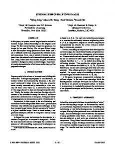
5.2. Effect of the Size of Statistical Feature Template on Classification Accuracies. Here, different features 𝐹00 , 𝐹10 , 𝐹11 of the 24000 error-diffused halftone images are used to test the effect of the size of statistical feature template. 𝐹00 , 𝐹10 , 𝐹11 are constructed using the corresponding class feature matrices 𝐺00 , 𝐺10 , 𝐺11 with deferent size 𝐿 × 𝐿 (𝐿 = 5, 7, 9, 11, 13, 15, 17, 19, 21, 23, 25). Figure 1 shows that the classification accuracy rate achieves the highest value when 𝐿 = 11, no matter which feature is selected for experiments. 5.3. Time-Consumption of the Classification. Now, the experiments are implemented to test the time-consumption of the error-diffused halftone image classification under the condition that the total number of samples is 24000 and 𝐿 = 11. It is well known that the time-consumption of the classification includes the training time and the testing time. From Table 4, we can know that the training time increases with the increase of the number of training samples; on the contrary, the testing time decreases with the increase of the number of training samples.
8
Advances in Multimedia 1 0.98 0.96 0.94 0.92 0.9 0.88 0.86 0.84 0.82 0.8 14000 15000 16000 17000 18000 19000 20000 21000 22000 L=5 L=7 L=9
L = 11 L = 13 L = 15
1 0.98 0.96 0.94 0.92 0.9 0.88 0.86 0.84 0.82 0.8 14000 15000 16000 17000 18000 19000 20000 21000 22000 L = 17 L = 19 L = 21
L = 23 L = 25
(a) Rates based on 𝐹00 (𝐿 = 5, 7, 9, 11, 13, 15)
(b) Rates based on 𝐹00 (𝐿 = 17, 19, 21, 23, 25)
0.9 0.89 0.88 0.87 0.86 0.85 0.84 0.83 0.82 0.81 0.8 14000 15000 16000 17000 18000 19000 20000 21000 22000
0.9 0.89 0.88 0.87 0.86 0.85 0.84 0.83 0.82 0.81 0.8 14000 15000 16000 17000 18000 19000 20000 21000 22000
L=5 L=7 L=9
L = 11 L = 13 L = 15
L = 17 L = 19 L = 21
L = 23 L = 25
(c) Rates based on 𝐹10 (𝐿 = 5, 7, 9, 11, 13, 15)
(d) Rates based on 𝐹10 (𝐿 = 17, 19, 21, 23, 25)
1 0.98 0.96 0.94 0.92 0.9 0.88 0.86 0.84 0.82 14000 15000 16000 17000 18000 19000 20000 21000 22000
1 0.98 0.96 0.94 0.92 0.9 0.88 0.86 0.84 0.82 0.8 14000 15000 16000 17000 18000 19000 20000 21000 22000
L=5 L=7 L=9
L = 11 L = 13 L = 15
(e) Rates based on 𝐹11 (𝐿 = 5, 7, 9, 11, 13, 15)
L = 17 L = 19 L = 21
L = 23 L = 25
(f) Rates based on 𝐹11 (𝐿 = 17, 19, 21, 23, 25)
Figure 1: Classification accuracy rates based on deferent features with deferent sample size.
To compare the time-consumption of the classification method proposed in this paper with other algorithms, such as the backpropagation (BP) neural network, radial basis function (RBF) neural network, and support vector machine (SVM), all the experiments are implemented using 𝐹10 , which is divided into two parts: 12000 training samples and 12000 testing samples (𝐿 = 11). From the digits listed in Table 5,
we can know that SR achieves the minimal summation of the training and testing time. In addition, Table 5 implies that the time-consumption of classifiers based on neural networks, such as the classifier based on RBF or BP, are much more than that of other algorithms, especially SR. This is because these neural network algorithms essentially use gradient descent methods to
Advances in Multimedia
9 Table 5: Time-consumption of different algorithms (in second). ML 110.42 1.2000
Training time Testing time
RBF 76.390 276.00
BP 2966.7 3.6000
SVM 49.297 62.400
SR 43.9337 6.3161
Table 6: Classification accuracy rates under different variances (%). Variance 0.01 0.10 0.50 1.00
14000 95.570 95.370 94.580 93.060
15000 95.422 95.233 94.522 93.067
16000 95.425 95.188 94.600 93.013
17000 95.529 95.157 94.671 93.343
18000 95.217 94.867 94.567 93.200
19000 98.440 98.200 98.320 96.980
20000 98.200 98.000 98.225 97.175
21000 98.033 97.767 98.033 96.800
22000 97.950 98.000 98.550 97.350
Table 7: Classification accuracy rates using other algorithms under different variances. Variance 0.01 0.10
ECF + BP 89.5000 88.1333
LMS + Bayes 88.7577 78.4264
ML 97.9981 96.8315
Variance 0.50 1.00
ECF + BP 79.7333 61.5000
LMS + Bayes 40.2682 33.8547
ML 82.9169 64.3861
optimize the associated nonconvex problems, which are well known to converge very slowly. However, the classifier based on SR performs the classification task through computing the square of the distance between each testing sample and different class-centroids directly. Hence, the time-consumption of it is very cheap.
such as image scaling and rotation, in the process of errordiffused halftone image classification.
5.4. The Experiment of Noise Attack Resistance. In the process of actual operation, the error-defused halftone images are often polluted by noise before the inverse transform. In order to test the ability of SR to resist the attack of noise, different Gaussian noises with mean 0 and different variances are embedded into the error-defused halftone images. Then classification experiments have been done using the algorithm proposed in this paper and the experimental results are listed in Table 6. According to Table 6, the accuracy rates decrease with the increase of the variances. As compared with the accuracy rates listed in Table 7 achieved by other algorithms, such as ECF + BP, LMS + Bayes, and ML, we find that our classification method has obvious advantages in resisting the noise.
Acknowledgments
6. Conclusion This paper proposes a novel algorithm to solve the challenging problem of classifying the error-diffused halftone images. We firstly design the class feature matrices, after extracting the image patches according to their statistical characteristics, to classify the error-diffused halftone images. Then, the spectral regression kernel discriminant analysis is used for feature dimension reduction. The error-diffused halftone images are finally classified using an idea similar to the nearest centroids classifier. As demonstrated by the experimental results, our method is fast and can achieve a high classification accuracy rate with an added benefit of robustness in tackling noise. A very interesting direction is to solve the disturbance, possibly introduced by other attacks
Competing Interests The authors declare that they have no competing interests.
This work is supported in part by the National Natural Science Foundation of China (Grants nos. 61170102, 61271140), the Scientific Research Fund of Hunan Provincial Education Department, China (Grant no. 15A049), the Education Department Fund of Hunan Province in China (Grants nos. 15C0402, 15C0395, and 13C036), and the Science and Technology Planning Project of Hunan Province in China (Grant no. 2015GK3024).
References [1] Y.-M. Kwon, M.-G. Kim, and J.-L. Kim, “Multiscale rank-based ordered dither algorithm for digital halftoning,” Information Systems, vol. 48, pp. 241–247, 2015. [2] Y. Jiang and M. Wang, “Image fusion using multiscale edgepreserving decomposition based on weighted least squares filter,” IET Image Processing, vol. 8, no. 3, pp. 183–190, 2014. [3] Z. Zhao, L. Cheng, and G. Cheng, “Neighbourhood weighted fuzzy c-means clustering algorithm for image segmentation,” IET Image Processing, vol. 8, no. 3, pp. 150–161, 2014. [4] Z.-Q. Wen, Y.-L. Lu, Z.-G. Zeng, W.-Q. Zhu, and J.-H. Ai, “Optimizing template for lookup-table inverse halftoning using elitist genetic algorithm,” IEEE Signal Processing Letters, vol. 22, no. 1, pp. 71–75, 2015. [5] P. C. Chang and C. S. Yu, “Neural net classification and LMS reconstruction to halftone images,” in Visual Communications and Image Processing ’98, vol. 3309 of Proceedings of SPIE, pp. 592–602, The International Society for Optical Engineering, January 1998.
10 [6] Y. Kong, P. Zeng, and Y. Zhang, “Classification and recognition algorithm for the halftone image,” Journal of Xidian University, vol. 38, no. 5, pp. 62–69, 2011 (Chinese). [7] Y. Kong, A study of inverse halftoning and quality assessment schemes [Ph.D. thesis], School of Computer Science and Technology, Xidian University, Xian, China, 2008. [8] Y.-F. Liu, J.-M. Guo, and J.-D. Lee, “Inverse halftoning based on the Bayesian theorem,” IEEE Transactions on Image Processing, vol. 20, no. 4, pp. 1077–1084, 2011. [9] Y.-F. Liu, J.-M. Guo, and J.-D. Lee, “Halftone image classification using LMS algorithm and naive Bayes,” IEEE Transactions on Image Processing, vol. 20, no. 10, pp. 2837–2847, 2011. [10] D. L. Lau and G. R. Arce, Modern Digital Halftoning, CRC Press, Boca Raton, Fla, USA, 2nd edition, 2008. [11] Image Dithering: Eleven Algorithms and Source Code, http:// www.tannerhelland.com/4660/dithering-elevenalgorithmssource-code/. [12] R. A. Ulichney, “Dithering with blue noise,” Proceedings of the IEEE, vol. 76, no. 1, pp. 56–79, 1988. [13] Y.-H. Fung and Y.-H. Chan, “Embedding halftones of different resolutions in a full-scale halftone,” IEEE Signal Processing Letters, vol. 13, no. 3, pp. 153–156, 2006. [14] Z.-Q. Wen, Y.-X. Hu, and W.-Q. Zhu, “A novel classification method of halftone image via statistics matrices,” IEEE Transactions on Image Processing, vol. 23, no. 11, pp. 4724–4736, 2014. [15] D. Cai, X. He, and J. Han, “Efficient kernel discriminant analysis via spectral regression,” in Proceedings of the 7th IEEE International Conference on Data Mining (ICDM ’07), pp. 427– 432, Omaha, Neb, USA, October 2007. [16] D. Cai, X. He, and J. Han, “Speed up kernel discriminant analysis,” The International Journal on Very Large Data Bases, vol. 20, no. 1, pp. 21–33, 2011. [17] M. Zhao, Z. Zhang, T. W. S. Chow, and B. Li, “A general soft label based Linear Discriminant Analysis for semi-supervised dimensionality reduction,” Neural Networks, vol. 55, pp. 83–97, 2014. [18] M. Zhao, Z. Zhang, T. W. S. Chow, and B. Li, “Soft label based Linear Discriminant Analysis for image recognition and retrieval,” Computer Vision & Image Understanding, vol. 121, no. 1, pp. 86–99, 2014. [19] L. Zhang and F.-C. Tian, “A new kernel discriminant analysis framework for electronic nose recognition,” Analytica Chimica Acta, vol. 816, pp. 8–17, 2014. [20] B. Gu, V. S. Sheng, K. Y. Tay, W. Romano, and S. Li, “Incremental support vector learning for ordinal regression,” IEEE Transactions on Neural Networks and Learning Systems, vol. 26, no. 7, pp. 1403–1416, 2015.
Advances in Multimedia
International Journal of
Rotating Machinery
Engineering Journal of
Hindawi Publishing Corporation http://www.hindawi.com
Volume 2014
The Scientific World Journal Hindawi Publishing Corporation http://www.hindawi.com
Volume 2014
International Journal of
Distributed Sensor Networks
Journal of
Sensors Hindawi Publishing Corporation http://www.hindawi.com
Volume 2014
Hindawi Publishing Corporation http://www.hindawi.com
Volume 2014
Hindawi Publishing Corporation http://www.hindawi.com
Volume 2014
Journal of
Control Science and Engineering
Advances in
Civil Engineering Hindawi Publishing Corporation http://www.hindawi.com
Hindawi Publishing Corporation http://www.hindawi.com
Volume 2014
Volume 2014
Submit your manuscripts at http://www.hindawi.com Journal of
Journal of
Electrical and Computer Engineering
Robotics Hindawi Publishing Corporation http://www.hindawi.com
Hindawi Publishing Corporation http://www.hindawi.com
Volume 2014
Volume 2014
VLSI Design Advances in OptoElectronics
International Journal of
Navigation and Observation Hindawi Publishing Corporation http://www.hindawi.com
Volume 2014
Hindawi Publishing Corporation http://www.hindawi.com
Hindawi Publishing Corporation http://www.hindawi.com
Chemical Engineering Hindawi Publishing Corporation http://www.hindawi.com
Volume 2014
Volume 2014
Active and Passive Electronic Components
Antennas and Propagation Hindawi Publishing Corporation http://www.hindawi.com
Aerospace Engineering
Hindawi Publishing Corporation http://www.hindawi.com
Volume 2014
Hindawi Publishing Corporation http://www.hindawi.com
Volume 2014
Volume 2014
International Journal of
International Journal of
International Journal of
Modelling & Simulation in Engineering
Volume 2014
Hindawi Publishing Corporation http://www.hindawi.com
Volume 2014
Shock and Vibration Hindawi Publishing Corporation http://www.hindawi.com
Volume 2014
Advances in
Acoustics and Vibration Hindawi Publishing Corporation http://www.hindawi.com
Volume 2014