CLASSIFICATION OF MACHINE OPERATIONS BASED ON GROWING NEURAL MODELS AND FUZZY DECISION Gancho Vachkov Department of Reliability–based Information Systems Engineering Faculty of Engineering, Kagawa University Hayashi-cho 2217-20, Takamatsu City, 761-0396 Kagawa, Japan E-mail:
[email protected]
KEYWORDS Growing Neural Models, Neural-Gas Learning, Information Compression, Classification, Fuzzy Decision, Evaluation of Machine Operations. ABSTRACT In this paper, a novel approach to analysis and classification of complex machine operations is presented. The available data sets from different machine operations are first compressed and saved in the form of neural models that are called compressed information models (CIM). Here an original algorithm for unsupervised learning is proposed. It creates the so called growing neural models in a sense that the number of neurons is gradually increasing (growing) during the learning process, until predetermined model accuracy (the “average minimum distance”) is satisfied. The proposed algorithm has much faster convergence compared with the classical neural-gas learning that uses preliminary fixed number of neurons. A special Knowledge Base classification scheme is also proposed in the paper. It uses a fuzzy decision block for computing the difference degree between each CIM in the Knowledge Base with the CIM of the current machine operation. The fuzzy inference procedure uses two parameters for comparison the CIMs, namely the decision the Center-of-Gravity and the General Size of the CIM. An example for classification of 45 specially generated operations from a diesel engine of a hydraulic excavator is used to demonstrate the whole proposed technology and its applicability. This fuzzy classification scheme is also able to discover new operations that significantly differ from all previously known operations. INTRODUCTION Many industrial systems and complex machines, such as chemical and power plants, hydraulic excavators and other construction machines often work under different operating conditions, depending on the load, raw material characteristics, ambient temperature etc. Basically, such machines and systems are equipped with different sensors that are used for data acquisition in Proceedings 21st European Conference on Modelling and Simulation Ivan Zelinka, Zuzana Oplatková, Alessandra Orsoni ©ECMS 2007 ISBN 978-0-9553018-2-7 / ISBN 978-0-9553018-3-4 (CD)
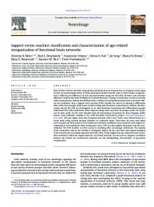
order to provide information about the daily operation of the system. This information is obtained in the form of large “raw data sets” which are further used for different types of off-line analysis, such as performance evaluation, classification and fault diagnosis, in order to detect possible deterioration trends or malfunctions and make respective decisions. The example, shown in the following Fig. 1. is from different operating conditions of the turbo diesel engine of a hydraulic excavator. It is easy to notice that each operation form a kind of “cloud” in the parameter space with specific shape and location in the space. Fuel Consumption 1
Heavy Load
0.8 0.6
Fault
Normal Load
0.4 0.2
Idling
Light Load
0 0
0.2
0.4
0.6 0.8 1 Engine Speed [rpm]
Figure 1: Example of Five Diffeent Operations of a Turbo Diesel Engine However if many operation data are collected over a long period of time (many days or months of operation) it is not easy task even for an experienced operator to analyse and classify them into a number of predefined groups of typical operations or as “new” or even “strange” (possibly abnormal or faulty) operations. The complexity of the problem arises from the fact that we have to analyse, compare and classify huge data sets to each other rather than classify single patterns (single data points in the feature space), as in the standard classification problem (Bishop, 1995; Bezdek et al. 2005). In the sequel of this paper we explain a novel approach to classification of large data sets. It is based on a preliminary information compression by use of special unsupervised learning algorithm for neural models, combined with fuzzy decision procedure for computing the difference degree between the neural models.
INFORMATION COMPRESSION BY USE OF NEURAL MODELS When a large number of “raw” data are collected for each machine operation, it is a good idea to initially preprocess by converting the raw data set into a more compact form, further called compressed information model (CIM). However such information compression procedure should be done carefully so that to preserve as much as possible the original data structure and the local density distribution of the data in the high dimensional parameter space. The learning methods for information compression generally belong to the group of the competitive unsupervised learning methods and algorithms (Bishop, 1995; Kohonen, 2001; Martinetz et al. 1993; Kasabov, 2001; Fritzke, 1994). Widely used are the SelfOrganized (Kohonen) Maps (Kohonen, 2001) and the Neural Gas Algorithm (Martinetz et al. 1993; Fritzke, 1994). Because of their unsupervised nature, these methods are pure “data-driven” learning techniques, which try to locate the neurons from the neural model in the densest area of the input space. As a result of the unsupervised learning, the large amount of M data is replaced by much smaller number of N neurons (N AVmin0; DEVn = ⎨ n = 1,2,..., N ⎩0, otherwise;
(7)
The Voronoi polygon with the biggest deviation DEV max will be the first (most urgent) candidate for correction, by receiving (at keast) one additional neuron. The main computation steps of the Growing-type Learning Algorithm are given below. The algorithm starts with a small initial number N o of neurons: N = N o ≥ 2 . Step 1. Perform the standard fixed-type neural-gas learning algorithm as in (Vachkov, 1996a) by using the complete set of all M data. As a result, the centers of all
N neurons in the K-dimensional [Ci1 , Ci 2 ,..., C iK ], i = 1,2,..., N are determined;
space
Step 2. Analyse the performance of the current neural model with N neurons for the complete set of M data by computing AVmin from (5). Step 3. Check for the stopping condition: If AVmin ≤ AVmin0 , then the algorithm stops (a satisfactory neural model with N neurons is created); otherwise continue to Step 4. Step 4. Analyse the current model-quality of each Voronoi polygon, as follow: Compute the Mean Distances MDn , n = 1,2,..., N for each neuron by using (6); - Compute the Deviations DEVn , n = 1,2,..., N by (7); - Sort the deviations DEVn for all N neurons in a descending order, from DEV max to DEV min . - Then the following decision is made: “The model quality of the Voronoi polygon where the neuron n * with the highest deviation: DEV max = DEV is located, n*
should be improved by inserting one or more additional neurons in its area.” Therefore, define the number mn* < M , as well as the list of all data points in this polygon n * . Step 5. Growing Step: insert a small number of neurons N ad ≥ 1 in the area of polygon n * for further learning. The initial positions (centers) of these additional neurons are set to coincide with randomly selected data from the same polygon. In the most often cases, only one additional neuron is inserted in the polygon n * , i.e N ad = 1 . Step 6. Perform again the fixed-type unsupervised learning algorithm as in Step 1, but for the highly reduced case of only N ad + 1 neurons and for the subset of only mn* data points, which are located in this Voronoi polygon n * . Note that the old neuron from this polygon is also included in this reduced number of Nad + 1 neurons that have to be trained. Step 7. Update the total number of the neurons for the current neural model: N ← N + N ad and Go to Step 2. An illustration of how the proposed growing-type learning algorithm works is given in the following Fig. 3. Here the first two consecutive epochs are only shown, starting with an initial number of N o = 2 neurons and adding one new neuron ( N ad = 1 ) at each consecutive Epoch. With a pre-deermined accuracy of AVmin0 = 0.02, the growing neural gas algorithm runs 31 epochs in total and finally produces a growing neural model with N = 32 neurons. This model was already displayed in Fig. 2 from the previous Section.
2 Neurons
1
P2
AVmin = 0.0638
Parameter Base
Fuzzy Rule Base
800 Raw Data
0.8
Fuzzy Decison
0.6
Knowledge Base (KB)
0.4
Fuzzy Decision Unit
(Difference Degree DD)
Avmin = 0.0682
.
0.2
Compressed Model (CIM) of a New Operation
0 0
0.2
0.4
0.6
0.8
a)
P1
1
3 Neurons
Figure 5: Block Diagram of the Proposed Knowledge based Fuzzy Inference System
1
AVmin = 0.0638
P2 0.8
AVmin = 0.0672 AVmin = 0.0578
0.6 0.4 0.2
800 Raw Data
0 0
b)
0.2
0.4
0.6
0.8
P1 1
Figure 3:Illustration of the first two Epochs from the Growing Neural Gas Algorithm The next Fig. 4. shows te convergence of the growingtype neural gas learning algorithm for the same example. As seen, the AVmin steadily decreases with the number of neurons (number of Epochs).
Here the Knowledge Base KB consists of a collection of CIMs for typical (known) operations of the machine, while the new operation (to be classified) is presented as an additional CIM, as shown in the Figure. The Fuzzy Rule Base (FR Base) and the Parameter Base in Fig. 5. are necessary elements of the Fuzzy Inference system, which makes a fuzzy evaluation by computing the Difference Degree (DD) between the CIM from the new operation (denoted as Model A) and each of the CIMs from the KB (denoted as Model B). We assumed here a two-dimensional fuzzy inference procedure: D = F ( X 1, X 2) which uses the following two parameters, namely the Center-of-Gravity Distance (X1) and the Model-Size Difference (X2), as shown below:
COGDAB ≡ X 1 =
AVmin 0.07
K
∑ [ COG j =1
A
( j ) − COGB ( j )] 2
(9)
Convergence Rate 0.06
MSDAB ≡ X 2 =
0.05
K
∑[ Z j =1
A
( j ) − Z B ( j )] 2
(10)
0.04
The assumed in this paper FR Base is shown in Fig. 6:
0.03
Fuzzy Rule Base: D = F(X1, X2)
X2
0.02 0.01 0
5
10
15
20
25
30
35
Neurons
Figure 4: The Convergence Curve of the Growing Neural Gas Algorithm with the Epochs (Neurons) THE FUZZY DECISION BLOCK FOR CLASSIFICATION OF OPERATIONS By use of the above learning algorithm, many available data sets from different operations could be compressed as respective CIMs for a consequent comparison, evaluation and classification. Here the fuzzy systems for pattern recognition and classification are quite flexible and therefore widely used for such purpose (Bezdek, 2005). In this paper we propose a specialized Knowledge based Fuzzy Inference system (called Fuzzy Decision Block) for classification of compressed operations (CIMs). The block diagram of the system is shown in Fig. 5.
VB
DIF
DIF
VDIF
VDIF
VDIF
BG
DIF
DIF
DIF
VDIF
VDIF
Model Size MD Difference
SIM
SIM
DIF
DIF
VDIF
SM
VSIM
SIM
SIM
DIF
DIF
VS
EQ
VSIM
SIM
DIF
DIF
VS
SM
MD
BG
VB
.
COG Distance
X1
Figure 6: The Fuzzy Rule Base for Fuzzy Decision An example of one concrete Fuzzy Rule is given below: IF( X1 is SM AND X2 is BG ) THEN D is DIF (11) Here the following 5 linguistic variables were assumed for the input parameters X1 and X2: VS = Very Small; SM = Small; MD = Medium; BG = Big and VB = Very Big.
The consequent D in the fuzzy rule (11) denotes the fuzzy set for the Degree of Difference DD which includes the following 5 linguistic variables: EQ = Equal; VSIM = Very Similar; SIM = Similar; DIF = Different; VDIF = Very Different. Triangular membership functions for the input parameters X1 and X2 were assumed, as shown in Fig. 7.
1
P2
1.0
Very Small
0.4
Small
Medium
Big
1.0
0.2
0.3
0.4
0.5 X1max
X1=0.23
Small
Medium
Big
f2 = 0.40
X1
Very Big
Model Size Difference
0.0 0.05
b)
X2min
22-24 10-12
0.10
0.15
0.20
X2 = 0.17
4-6
1-3
0.6
0.8
7-9
0
Membership Value Very Small
16-18
19-21
Idling
0.0
f2
25-27
13-15
Very Big
Center-ofGravity Distance
a)
37-39
0.2
f1 = 0.70
0.1
Fault
40-42
28-30
0
X1min
31-33
34-36
0.6
Membership Value
f1
43-45
0.8
0.25 X2max
X2
0.4
1
P1
Figure 8: Locations and Numbers of all Operations used for the Classification Large ball-type curve symbols in Fig. 8. denote the five core operations (from the Knowledge Base), while all other 12 curve symbols with smaller size denote the deviated operations by simulation. The deviation of the COG for the LL, NL and HL was by amount of +α and −α for P1 and by + β and − β for P2, with α = 0.1 and β = 0.1 . In addition, the general size GS of each operation (including the main operations LL, NL and HL) has been changed twice, as follows: a smaller size GS1 = 0.8GS by 20% and a larger size GS2 = 1.2GS by 20%. The main 3 operations LL, NL and HL, with normal size GS are numbered in Fig. 8. as 1, 16 and 31, respectively. . The results from the classification are shown in the next Fig. 9., separately for the cases of LL, NL and HL.
Figure 7: Triangular Membership Functions for the Input Parameters X1 and X2 of the Fuzzy Decision
Difference Degree (DD) 0.6
The standard product-operation for fuzzy inference, as well as the weighted average method for defuzzification were used here for the final computation of the difference degree DD.(details omitted).
Comparison with the Standard "Light Load" Operation
0.5 0.4 Threshold 0.3 0.2
CLASSIFICATION OF OPERATIONS FROM A TURBO DIESEL ENGINE In this Section we show how the whole technology, consisting of information compression and fuzzy decision works for classification of various operations of a turbo diesel engine of a hydraulic excavator. For this purpose we use the available data from 4 main operations of the diesel engine under different loads, namely: Light Load (LL), Normal Load (NL), Heavy Load (HL) and Idling. In addition, data from another (possibly faulty) operation was also used, named as Fault. Therefore all these 5 core operations were included in the Knowledge Base of the classification system., according to Fig. 5. Various operations for classification were produced by slightly moving the original data sets for LL, NL and HL to different locations in the parameter space. We also changed their spread (size) by a special simulation program. Finally, 45 operations in total were obtained, (including the LL, NL and HL), as shown in Fig. 8.
0.2
Deviations from "Light Load" Operations
0.1 0 0
2
4
6
8
10
12
14
16
Data Sets (Operations)
a)
Difference Degree (DD) 0.6
Comparison with the Standard "Normal Load" Operation
0.5 0.4
Threshold
0.3 0.2
Deviations from "Normal Load" Operations
0.1 0 16
b)
18
20
22
24
26
28
Data Sets (Operations)
30
Difference Degree (DD) 0.6
operations are compared with those from a preliminary created Knowledge Base of typical operations. The difference degree DD between them is computed by a specialized fuzzy decision block. The future research in this direction is aimed at improving the “plausibility” of the classification by appropriately tuning all the internal parameters.
Comparison with the Standard "Heavy Load" Operation
0.5 0.4 Threshold 0.3 0.2
Deviations from "Heavy Load" Operations
0.1 0 30
32
34
36
38
40
42
44
REFERENCES 46
Data Sets (Operations)
c)
Figure 9: Classification Results for All Operations: a) Light Load; b) Normal Load; c) Heavy Load A threshold of 0.35 was set in this case for classifying the operations in two groups, as follows: belonging to the respective main operation (when the difference degree DD < 0.35) or not belonging to this operation (if DD > 0.35). We leave the sensitive choice of the threshold to the experience of the human operator. In Fig. 10. two additional (artificially generated) operations are shown, named as Op_X and Op_Y. They have unknown status and (as seen) are largely different from the main operations: LL, NL, HL, Idling and Fault, but may have some similarities with some of them , namely: Op_X is somewhere between HL and Idling; OP_Y is somewhere between LL and Fault. Our classification system produced the following result: Op_X is the closest to HL with DD = 0.52, but the assumed threshold of 0.35 “rejects” this decision; Op_Y is the most closest to LL with DD = 0.66, but it is also rejected by the given threshold. Therefore, these two operations are finally classified as “new” and quite different operations. They could be included as “new members” of the enlarged Knowledge Base for classification of future operations. Thus the Knowledge Base will gradually grow (as cumulative experience). 1
HL
P2
Fault
AUTHOR BIOGRAPHY
0.8 0.6 0.4
Op_X
NL
Op_Y
0.2
LL
Idling 0 0
0.2
0.4
0.6
0.8
P1
Bezdek, J.C.; J. Keller; R. Krisnapuram; and N.R. Pal. 2005. “Fuzzy Models and Algorithms for Pattern Recognition and Image Processing”. The Handbooks of Fuzzy Sets Series. Printed in the U.S.A., 288-303. Bishop, Ch.M. 1995. Neural Networks for Pattern Recognition, Oxford University Press, Oxford, New York, 1995, 164-177. Fritzke, B. 1994. “Growing Cell Structures – a Self-organizing Network for Unsupervised and Supervised Learning, Neural Networks, Vol. 7, No. 9, pp. 1441-1460, 1994. Huang G.-B., P. Saratchandran and N. Sundarajan, 2005. “A Generalized Growing and Pruning RBF (CGAP-RBF) Neural Network for Function Approximation”, IEEE Trans. on Neural Networks, vol. 16, No. 1, 57-67, 2005. Kasabov, N. 2001. Evolving Fuzzy Neural Networks for Online Supervised/Unsupervised, Knowledge-based Learning, IEEE Trans. on SMC – part B, Cybernetics, Vol. 31, No. 6, 902-928. Kohonen, T. 1997. Self-Organizing Maps, 2nd Edition, Springer Verlag. 105-161. Martinetz, T.; S. Berkovich; and K. Schulten. 1993. “NeuralGas Network for Vector Quantization and Its Application to Time-series Prediction”, IEEE Trans. on Neural Networks, Vol. 4, No.4, 558-569. Vachkov, G. 2006, “Fault Diagnosis of Complex Systems Based on Modular Knowledge Base and Information Compression, Proc. of the 20th European Conference on Modelling and Simulation, ECMS 2006, Bonn, ASankt Augustin, Germany, May 28-31, 112-117. Vachkov, G. 2006. “Recognition of Different Operating States in Complex Systems by Use of Growing Neural Models”, Proc. of the 2-nd IEEE Int. Symposium on Evolving Fuzzy Systems, EFS’06, Ambleside, Lake District, UK, 7-9 Sep. 2006, 80-85.
1
Figure 10:Two Additional (Unknown) Operations CONCLUSIONS In this paper we presented a new two-stage approach to classification of large data sets from different machine operations. First of all the data sets are converted into compact neural models (CIMs) by the growing neural gas learning algorithm. Then the CIMs from new
GANCHO L. VACHKOV was born in Bulgaria in 1947. He graduated from the Technical University in Sofia, Department of Industrial Control in 1970 and obtained a Ph.D. degree in the field of Analysis of Complex Technological Systems in 1978. From 1970 until 1995 he was with the Department of Automation of Industry at the University of Chemical Technology and Metallurgy in Sofia. Since September, 1996 he has been working in Japan, in the following Universities: Kitami Institute of Technology (1996-1998); Nagoya University, Dept. of Micro-System Engineering (1998-2002) and Kagawa University, Dept. of Reliability-based Information Systems Engineering (2002 – present). Research interests and results of G. Vachkov are in the wide area of Computational Intelligence, with a focus on the: Learning Algorithms for Fuzzy and Neural Modeling, Identification and Control, Intelligent Data Processing for Evaluation of Systems Performance and Fault Diagnosis. His e-mail address is :
[email protected].