Classification of Stellar Spectral Data Using SVM Fei Xing and Ping Guo Department of Computer Science Beijing Normal University, Beijing, 100875, P.R.China
[email protected];
[email protected]
Abstract. In this paper a new technique is developed on stellar spectral classification. Because stellar spectral data sets are usually extremely noisy, wavelet de-noising method is proposed to reduce noise first. Then the support vector machines (SVM) is used for the classification. Experimental results show that in most cases, there will be a better performance using this composite classifier than using SVM with principle component analysis data dimension reduction technique.
1
Introduction
Stellar spectral classification is an important part of automatic recognition of astronomical spectra. Because classifying the spectral data of great bulk manually is a tough job, the technology of automatic and accurate classification on spectral data should be developed. To automatically recognize stellar spectra, we should build the classifier with training samples first. There are many classification techniques in this research field, among them discriminant analysis is one of the supervised learning classifier building techniques. Quadratic discriminant analysis (QDA) is widely used if sufficient training samples could be supplied [1, 2]. Unfortunately, sometimes training samples are usually hard to acquire, and the dimensionality of spectral data is extremely high, thus the estimated covariance matrix will become singular. Linear discriminant analysis (LDA) could be used as one kind of regularization if the total number of samples is larger than the dimension of variables. The covariance matrix, in LDA, is substituted by common covariance matrix. However, in the case of small sample sizes, the common covariance matrix is also singular. To solve the small training sample with high-dimension setting problem, Regularized discriminant analysis (RDA) [3] could be applied. RDA adds the identity matrix as a regularization term to solve the problem in matrix estimation. But parameter optimization of RDA is time consuming. Artificial neural network (ANN) is also a good tool for pattern recognition, it has been successfully used in classification of stellar spectra [4]. Different network models are developed in recent years, the performance of them is data dependent. Support Vector Machines (SVM) [5] is a new technique for data classification, it has been used successfully in many object recognition applications [6–8].
SVM is known to generalize well even in high dimensional spaces under small training sample condition. This characteristic is appropriate for stellar spectral classification where such conditions are typically encountered.
2
Support Vector Machines
SVM was introduced by Vapnik in the late 1960s on the foundation of statistical learning theory [9]. In theory, the SVM classification can be traced back to the classical structural risk minimization (SRM) approach, which determines the classification decision function by minimizing the empirical risk. SVM uses linear model to implement nonlinear class boundaries through some nonlinear mapping the input vectors x into the high-dimensional feature space. The optimal separating hyperplane is determined by giving the largest margin of separation between different classes. For the two-class case, this optimal hyperplane bisects the shortest line between the convex hulls of the two classes. The data are separated by a hyperplane defined by a number of support vectors. The SVM attempts to place a linear boundary between the two different classes, and orient it in such a way that the margin is maximized. The boundary can be expressed as follows: (w · x) + b = 0,
w ∈ RN , b ∈ R,
(1)
where the vector w defines the boundary, x is the input vector of dimension N and b is a scalar threshold. The optimal hyperplane is required to satisfy the following constrained minimization as 1 min{ kwk2 } with 2
yi (w · xi + b) ≥ 1, i = 1, 2, . . . , l,
(2)
where l is the number of training sets. For a linearly non-separable case, the above formula can be extended by introducing a regularization parameter C as the measurement of violation of the constraints as follows: l l X 1 X min{ λi − λi λj yi yj (xi · xj )} 2 i,j=1 i=1
with
l X
yi λi = 0, 0 ≤ λi ≤ C, i = 1, 2, . . . , l,
(3)
i=1
where the λi are the Lagrangian multipliers and are nonzero only for the support vectors. Thus, hyperplane parameters (w, b) and the classifier function f (x; w, b) can be computed by optimization process. The decision function is obtained as follows: l X yi λi (x · xi ) + b}. (4) f (x) = sgn{ i=1
In cases where the linear boundary in input spaces will not be enough to separate two classes properly, it is possible to create a hyperplane that allows linear separation in the higher dimension. The method consists in projecting the data in a higher dimension space where they are considered to become linearly separable. The transformation into higher-dimensional feature space is relatively computation-intensive. A kernel can be used to perform this transformation and the dot product in a single step provided the transformation can be replaced by an equivalent kernel function. This helps in reducing the computational load and at the same time retaining the effect of higher-dimensional transformation. The kernel function K(xi , xj ) is defined as follows: K(xi , xj ) = φ(xi ) · φ(xj ).
(5)
There are some commonly used kernels: 1. Polynomial: K(xi , xj ) = [(xi · xj ) + 1]q 2. Radial basis: K(xi , xj ) = exp(−kxi − xj k2 /2σ 2 ) 3. Sigmoid: K(xi , xj ) = tanh(ν(xi · xj ) + c)
3
Experiments
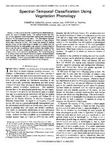
The stellar spectra used in our experiments are selected from Astronomical Data Center (ADC). We use 161 stellar spectra contributed by Jacoby et al. (1984). Ordered from highest temperature to lowest, the seven main stellar types are O, B, A, F, G, K, and M. The seven main types of stellar spectrum lines are shown in Fig. 1(a).
1
(b)
(a) 0.9
12
0.8
10 0.7
8 0.6
6 0.5
I
4 0.4
2 0.3
0 10
0.2
10
0 0.1
0 3500
0
−10
−10 −20
−20 4000
4500
5000
5500 Wavelength(Å)
6000
6500
7000
−30
7500
−30
−40
Fig. 1. (a) Seven main types of stellar spectra. (b) Distribution of stellar spectra in first three principal components space
The bootstrap technique [10] is applied in experiments. 161 samples are divided into two parts, 10 independent random samples drawn from each class are
Table 1. Mean and standard deviation of the classification accuracy of SVM, PCA+SVM and wavelet+SVM Methods SVM wavelet+SVM PCA+SVM CCR 81.66% 93.26% 81.30% STD 3.75 3.08 2.90
used to train the SVM classifier and the remaining samples are used as test samples to calculate correct classification rate (CCR). The experiment is repeated 25 times with random different partition and the mean and standard deviation of the classification accuracy are reported. In the tables presented in this paper, the classification accuracy is reported in percentage. The SVM is designed to solve two-class problems. For multi-class stellar spectra, a binary tree structure is proposed to solve the multi-class recognition problem. Usually two approaches can be used for this purpose [9, 11]: a) The one-against-all strategy to classify between each class and all the remaining. b) The one-against-one strategy to classify between each pair. We adopt the latter one for our multi-class stellar spectral classification, although needing more SVM to be applied, that allows the computing time to be decreased because the complexity of the algorithm depends strongly on the number of training samples. In the experiment, firstly original data is directly used as the input of SVM. Table 1 shows that direct classification using SVM could achieve 81.66% CCR. Because the stellar spectral data sets are extremely noisy, the classification rate of directly applying SVM is low. In order to raise the CCR, we propose to adopt wavelet de-noising method to reduce noise first. Wavelet transform, due to its excellent localization property, has become an important tool for de-noising. De-noising by wavelet thresholding was introduced by Donoho and Johnstone [12]. The basic method we use in the experiment involves two steps: 1). Calculate the wavelet coefficients. 2). Identify and zero out wavelet coefficients of the signal which are likely to be noise, remaining wavelet coefficients reserve important high pass features of the signal. Then the SVM is used for the final spectrum recognition (We denote this composite classifier which combines wavelet de-noising and SVM as wavelet+SVM). Table 1 indicates that this method could achieve 93.26% CCR and the smaller standard deviation than direct classification using SVM. According to the hypothesis tests (t-test) applied, the wavelet+SVM method has the mean of the classification accuracy in the validation set significantly (α=0.05) larger than direct classification using SVM (p-values equal to 1.97 × 10⁻⁸ ). Principal Component Analysis (PCA) [13] is a good tool for dimension reduction, data compression and feature extraction. As a comparison, we use the dimension reduced data with PCA as the input of SVM (We denote this method as PCA+SVM). The distribution of these eigen-spectra in first three principal components (PCs) space is shown in Fig. 1(b). From Fig. 2(a), we can find that the first 10 PCs just have only 0.43% reconstruction error, so we choose them to define a 10-dimensional subspace and map spectra on it to obtain 10-
dimensional vectors. Fig. 2(b) shows a comparison of the original spectrum to the PCA reconstructed spectrum and the wavelet denoised spectrum. 1 (a)
160
(b) 140
0.5
120
0 Eigenvalue
100
80
−0.5 60
−1
40
20
−1.5 0 −10
0
10
20
30
40 50 Eigenvalue index
60
70
80
90
100
−2
0
500
1000
1500
2000
2500
3000
Fig. 2. (a) Eigenvalue in decreasing order. (b) The de-noising result. Above line is original spectrum, middle line is with PCA (10 PCs reconstructed spectrum), bottom line is with wavelet de-noising
From Table 1, we can see that the performance of PCA+SVM is not very good. It’s even worse than direct classification with SVM. According to the hypothesis tests (t-test) applied, the PCA+SVM method has the mean of the classification accuracy in the validation set significantly (α=0.05) smaller than wavelet+SVM method (p-values equal to 2.01 × 10⁻¹⁰ ). The reason is that SVM can simulate a non-linear projection which can make linearly inseparable data project into a higher dimension space, where the classes are linearly separable. So data dimension has little influence on SVM. Discriminant analysis is one of the supervised learning classifier building techniques. We also compare QDA and LDA to SVM. The stellar spectrum data are drawn from standard stellar library for evolutionary synthesis and are the same from Ref. [14]. The data set consists of 457 samples and could be divided into 3 classes. The spectrum is of 1221 wavelength points covering the range 9.1 to 160000 nm. The experiments are conducted as in Ref. [14]. Table 2 shows that the performance of SVM is better than QDA and LDA. The higher CCR and lower standard deviation is achieved. Table 2. The classification accuracy comparison of QDA, LDA and SVM Methods QDA LDA SVM CCR 96.21% 94.88% 99.87% STD 0.84 0.47 0.18
4
Conclusions
In this paper, a new technique on stellar spectral recognition which combines wavelet and SVM is proposed in this paper. From the experiments we can see that the proposed classifier has a good performance. According to the hypothesis tests (t-test) applied, the classification results of the wavelet+SVM are better than either SVM alone or SVM with PCA data dimension reduction technique. Experiments have been done to demonstrate that the approach offers a very promising technique in automated process of stellar spectra.
Acknowledgements The research work described in this paper was fully supported by a grant from the National Natural Science Foundation of China (Project No. 60275002) and by National High Technology Research and Development Program of China (863 Program, Project No. 2003AA133060).
References 1. Aeberhard, S., Coomans, D., Vel, O. D.: Comparative Analysis of Statistical Pattern Recognition Methods in High Dimensional Settings. Pattern Recognition, 27 (1994) 1065–1077 2. Webb, A.: Statistical Pattern Recognition. Oxford University Press, London (1999) 3. Friedman, J. H.: Regularized Discriminant Analysis. J. Amer. Statist. Assoc., 84 (1989) 165–175 4. VonHippel, T., Storrie-Lombardi, L. J., Storrie-Lombardi, M.C., Irwin, M. J.: Automated Classification of Stellar Spectra - Part One - Initial Results with Aartificial Neural Networks. R.A.S. Monthly Notices, 269 (1994) 97–104 5. Cortes, C., Vapnik, V.: Support Vector Networks. Machine Learning, 20 (1995) 273–297 6. Dumais, S.: Using SVMs for Text Categorization. IEEE Intelligent Systems, 13 (1998) 21–23 7. Pontil, M., Verri, A.: Support Vector Machines for 3D Object Recognition. IEEE Trans. on Pattern Analysis & Machine Intelligence, 20 (1998) 637–646 8. Drucker, H., Wu, D., Vapnik, V.: Support Vector Machines for Spam Categorization. IEEE Trans. on Neural networks, 10 (1999) 1048–1054 9. Vapnik, V.: The Nature of Statistical Learning Theory. SpringerVerlag, New York (1995) 10. Efron, B., Tibshirani, R.: An Introduction to the Bootstrap. Chaoman & Hall, London (1993) 11. Weston, J., Watkins, C.: Support Vector Machines for Multi-Class Pattern Recognition. Proceedings of the Seventh European Symposium on Artificial Neural Networks, D-Facto, Brussels (1999) 219–224 12. Donoho, D. L.: De-noising by Soft-thresholding. IEEE Trans. on Information Theory, 41 (1995) 613–627 13. Jolliffe, I. T.: Principal Component Analysis. Springer-Verlag, New York (1986) 14. Wang, X., Xing, F., Guo, P.: Comparison of Discriminant Analysis Methods Applied to Stellar Data Classification. Proceedings of SPIE, Vol. 5286. SPIE, Bellingham WA (2003) 758–763