Classification support using confidence intervals Wilbert van Norden Defence Material Organisation CAMS – Force Vision Den Helder, the Netherlands
[email protected]
Fok Bolderheij Defence Material Organisation CAMS – Force Vision Den Helder, the Netherlands
[email protected]
cuts however, there is a strive to reduce the ship’s complements as well as the available training time. In short we observe that having a good and timely classification has become increasingly important as well as increasingly difficult to obtain; a decision support system is therefore needed. Having good classification solutions for all objects in the environment is important for obtaining and maintaining situation awareness. This paper describes how the system can combine measurements to automatically find a classification solution. In section two the background of this study is given as well as how this work is related to ongoing research. In section three the classification model that we use will be discussed briefly. Based on the modelling we use, section four will describe how confidence intervals can be constructed for any number of Gaussian distributed variables. These intervals are related to the mission information, which is described in section five. The implemented mission planner in which the classifiers operate is discussed in section six. Finally, sections seven and eight will outline future work and present the conclusions.
Abstract – In recent years the discrepancy between the required knowledge and the available knowledge for obtaining the situation awareness aboard Royal Netherlands Navy ships has increased. This paper presents a methodology to automatically classify objects in the mission environment based on user defined mission information in order to close this gap. The cornerstone of this methodology is the Confidence Interval (CI) based on Gaussian distributed measurements. To solve the classification problem effectively we describe how such a CI can be constructed for any number of variables. A mission planner has been implemented where operators can define a mission and where objects in the environment are automatically classified based on those mission parameters. Keywords: Classification, Reasoning with uncertainty.
1
Confidence
Catholijn Jonker Man-Machine Interaction Group Delft University of Technology Delft, the Netherlands
[email protected]
Interval,
Introduction
In recent years the classification process aboard naval warships has become increasingly difficult. There are several reasons for this. Firstly, because the operational theatre has changed from blue to littoral waters, which means that sensor performance is unpredictable due to rapidly changing meteorological conditions and due to the geographical conditions at the current location. The latter also enables hostile forces to stay hidden longer, which reduces reaction time what in turn makes the classification problem extremely difficult. Not only has the environment become more complex, the missions themselves have become more complex as well. Currently, missions involve peacekeeping, counter drug operations or enforcing trade embargos. These missions are also characterised by an asynchronous threat and much media attention, which have been proven to be of much influence during a recently held exercise ‘Noble Midas’ described in [1]. The first makes the classification itself harder whereas the latter gives high pressure not to make mistakes. A third aspect is the discrepancy between the knowledge available and required for the classification task. Where sensor systems are becoming increasingly complex, much knowledge is needed to properly set the sensor controls to operate optimally in any given situation. Due to budget
2
Background
The research presented in this paper is conducted based on the results of the STATOR1 project: a collaboration between the Royal Netherlands Naval College, the International Research Centre for Telecommunications and Radar of the Delft University of Technology and Thales the Netherlands. The focus of this project was the management of sensor suites and the fusion of the data provided by that sensor suite. The goal is to develop a decision support system where the operator can communicate with the sensor suite as a whole in operational terms. In so doing no technical settings are required directly from the operator. More detailed information on this overall concept can be found in [2].
2.1
Sensor Management
Previous research showed that the basis for sensor management is reducing uncertainty in the compiled picture, [3]. On the basis of the uncertainties residing in
1
295
STATOR: Sensor Tuning And Timing on Object Request
solution that reduces enough class uncertainty for deciding on appropriate actions in time. A good and timely solution as described here, places constraints on the modelling of the classification space. In other words, to answer the first question, the answers to the other two questions need to be taken into account. The next section will therefore discuss the details of a classification model in more detail.
this compiled picture, sensors could be tasked in order to reduce uncertainty as much as possible. Decisions the sensor manager needs to make are: 1) which task should be performed and 2) which sensor should be used for any of these tasks given the environment and mission constraints. Both questions are not easily answered. This paper will therefore focus on the first task of choosing the appropriate task to perform, also called sensor tasking. More specifically, this paper focuses on the sensor tasks that are required to optimise the classification of objects.
2.2
3
In this study we used the classification model described in [6]. This model uses three hierarchical classification levels. At the highest-level superclasses are defined. In our application these classes represent the different domains: air, surface, subsurface. Included in the superclasses are the sub-domains land and sea. The Venn diagram of this highest level is given in Figure 1.
Sensor Tasking
The goal of deploying sensors is to obtain and maintain a representation of the world in the command and control system. Such a representation, called (common) operational picture, consists of detected and/or expected objects. Sensors in general can measure a wide variety of attributes, amongst others: position, speed, acceleration, identity and classification. All mentioned attributes are important in the military work-domain. For most of these attributes uncertainty reduction seems quite straightforward. Reducing classification uncertainty however, is more difficult. In order to find a mechanism that can generate sensor function requests we need to further look at the classification process itself.
2.3
The Model
Classification
Having a correct and timely classification solution is of vital importance to mission success in any work-domain. Therefore, optimising the sensor suite to facilitate the classification process is equally important. Before this can be done however, we need to describe 1) how the classification space needs to be modelled, 2) what a good classification solution is and 3) what a timely solution is. The answer to the first question is described in more detail in section three, but here we will shortly state what classification is: classification tries to recognise the observed object in as much detail as possible. When this is done the object attribute type is accurately known in the (common) operational picture. A good classification is the solution where the uncertainty in the class information does not cause uncertainty in the risk; in this research the notion of risk from [4] is used. E.g., the distinction between two sea skimming missiles causes only a little reduction in risk uncertainty, distinguishing between an airliner and a fighter does reduce uncertainty in risk. Besides the advantage of risk uncertainty reduction, a good classification also improves on radar performance in tracking, [5]. In the military domain the starting point is to assume the worst-case scenario. With incoming objects this means that at a certain point in time precautionary actions must be taken. Before this happens, a classification solution could negate the necessity of actions thus preventing collateral damage. A timely solution is therefore the
Figure 1 Venn diagram of the five different domains. The middle level consists of generic classes such as fighters and helicopters. Finally, at the third level specific classes are described. The goal in the classification process is to assign a class at the appropriate level of detail as mentioned in the previous section. Since each class exists in an attribute space, we can map the available knowledge we have about an object onto the sets of classes and see where the best fit occurs. In order to do this, we need to know: 1) what the object looks like in such an attribute space; and 2) how uncertainty in single measurements can be combined to find the uncertainty regions in the multi-attribute space. In general, the measurement and its related uncertainty produce a confidence interval given a certain percentage; some value on that confidence interval is the actual value with the given percentage of probability. The amount of overlap between such a confidence interval and the class gives the amount of support the system has for a classification solution. Examples of classifying objects based on multiple kinematic attributes can be found in [7] and [8].
296
4
To solve equation (1) we use the definition of the error function (erf, equation (2)), to solve the integral over the Gaussian distribution. The definition of this erf-function can be found in [9]. Using equation (2) we can solve the boundary condition and we find equation (3) for the CIboundary. This however, is not enough to find the exact CI region. Finding that region means that we need to find all combinations of the variables that satisfy the boundary condition, equation (4).
Confidence Intervals
Reasoning about objects and comparing them with a database of known and expected classes means that confidence intervals (CI) need to be calculated on the basis of measurements. In this section we will first show how such CI’s are constructed for two and four variables based on a tracking example, note that this is only done because of the evocative nature of the tracking problem. We will then proceed by giving the general formulas for n variables.
4.1
pr (r ) pb (b) = pr ( µ r + ασ r ) ⋅ pb ( µb + ασ b)
Two variables
To solve equation (4) we define range as r = µ r + ρσ r
To solve the problem of where an object is in 2D Cartesian coordinates with a radar system, we have to combine range and bearing information. These measurements have an amount of uncertainty and the resulting Cartesian position has a resulting uncertainty region. For small uncertainties in the individual measurements a well fitting assumption can be made about the uncertainty region in Cartesian coordinates. When uncertainties increase, such assumptions become less accurate. An exact solution to find the boundaries of the CI becomes necessary in those cases. Let us look at the problem of finding the uncertainty region in Cartesian coordinates by combining uncertain range (r) and bearing (b). In this example a Gaussian distribution on both measurements is assumed. Since the conversion from polar coordinates to Cartesian coordinates is a standard mathematical operation, we will only look at the combinations of range and bearing that form the boundary of the CI. To find this CI-boundary we need to solve equation (1). Since we only look at the Gaussian distribution itself, we can say that this approach works for any combination of two Gaussian distributed variables.
and bearing as b = µb + βσ b . After basic mathematical operations we find equation (5).
ρ 2 + β 2 = 2α 2
pr (r ) ⋅ pb (b) ⋅ drdb = CI
erf 2
π α 2
x
2
e − t dt
b = µ b + 2σ b ⋅ erf with
4.2
(1)
(2) (3)
For notational purposes we define the following:
px r b
µx σx α
−1
t = [0...2π ]
(6)
Four variables
When reasoning about objects usually more than two variables are used. To illustrate this, we will include possible movement by the object from the previous example. This movement consist of a speed (s) and a course (c), both Gaussian distributed. Given the previous measurements of these four attributes we now want to find the CI-region at the next time step. To find this region we will again need to determine the boundary condition first, equation (7). Since we are solving the distribution, the solution can be used in any field. Note that the use of equation (7) assumes independency between the four variables, which does not hold in actual tracking problems. Since we only use the tracking example to illustrate how uncertainty regions can be calculated based on independent variables, we will discard these dependencies in this work. For actual tracking implementations, already developed tracking algorithms will be used.
0
= CI
( ) ( CI )⋅ cos(t )
r = µ r + 2σ r ⋅ erf −1 CI ⋅ sin (t )
µb −ασ b µr −ασ r
2
(5)
We then find equation (6) for the combinations of range and bearing that constitute the outer limits of the confidence interval. Using this equation we can easily draw the CI-region in Cartesian coordinates without making any assumptions on the shape of this region. In equation (6) the inverse error function is denoted by erf −1 .
µb +ασ b µr +ασ r
erf (x ) =
(4)
Gaussian probability density function of variable x; Range; Bearing; Mean value of variable x; Standard deviation of variable x; Boundary value.
297
µb +ασ b
µr +ασ r
pb db ⋅
pr dr µr −ασ r
µb −ασ b
µs +ασ s µ s −ασ s
erf 4
µc +ασ c
pc dc = CI
p s ds
α 2
Table 1 Last known kinematic information
(7)
µ
µc −ασ c
= CI
Range Bearing Speed Course
(8)
Similar to equation (2) for two variables we find equation (8) as the relation between CI and the CI-boundary. When we define: r = µ r + ρσ r ; s = µ s + ϑσ s ;
b = µb + βσ b ;
In Figure 2 and Figure 3 the squares indicate the position where the probability density is at a maximum for the current time step given the range and bearing. The triangles indicate the maximum probability density for the next time step given the course and speed. In the two previous sections we used a tracking example to illustrate how Gaussian distributed measurements can be combined to find a combined CI-region. In the next section we will give the formulas in a more generic way.
c = µ c + γσ c ;
we find equation (9).
ρ 2 + β 2 + ϑ 2 + γ 2 = 4α 2
(9)
Now, define A 4 = ρ 2 + β 2 and B 4 = ϑ 2 + γ 2 which
Range:10+/-3. Bearing:90+/-10. Speed:10+/-1. Course:180+/-8. 4
produces A2 = 2α ⋅ sin( p ) and B 2 = 2α ⋅ cos( p ) . This in turn produces: ρ = 2α ⋅ sin ( p ) ⋅ sin (t ) ; β = 2α ⋅ sin ( p ) ⋅ cos(t ) ϑ = 2α ⋅ cos( p ) ⋅ sin (t ) ; γ = 2α ⋅ cos( p ) ⋅ cos(t )
2 0 -2 y-coordinate
-4 -6 -8
p = 0...2π and t = 0...2π .
with
2σ 3 10 1 8
10 90 10 180
-10 -12
Now, assume the example as given in Table 1. Using equation (6) we find the uncertainty region (the dotted line), shown in Figure 2, given the available range and bearing measurements. Using the results from this section we can also find all possible positions at the next time step, indicated by the solid lines in Figure 2. To find the entire CI-region we simply take the outer limits of all solid lines, producing Figure 3.
-14 -16
4
6
8
10 x-coordinate
12
14
16
18
Figure 3 The CI-regions for the current position and the outer limits of the next expected position.
4.3
n Variables
In the previous sections we discussed reasoning with two or four variables, illustrated with a tracking example. Note that this approach is not relevant for actual tracking due to the relatively small uncertainties and the high update rates. We choose this description because of its evocative nature. However, in the tracking example the use of two or four variables seems enough whereas in the classification space more combinations of multiple attributes need to be made to come to a good classification solution as described in section 2.3.
Range:10+/-3. Bearing:90+/-10. Speed:10+/-1. Course:180+/-8. 4 2 0 -2
y-coordinate
2
-4 -6 -8 -10 -12 -14 -16
n
2
4
6
8
10 x-coordinate
12
14
16
∏
18
i =1
µ xi +ασ xi
( )
p xi ⋅ dxi = CI → α = 2 ⋅ erf −1 n CI
µ xi −ασ xi
xi = µ xi + ξ xi σ xi
Figure 2 Given the CI of the current position, the CI for the next position can be found by combining all solid lines.
298
(10) (11)
Utilising the combination of the CI-region found using equation (13) with classes in the same attribute space we can determine which attribute’s uncertainty causes the most classification uncertainty. This can be used in sensor management concepts to generate sensor function requests in order to reduce this uncertainty, the second stage of the three-stage-sensor manager described in [10].
α against the number of variables for different CI 4
3.5
Boundary value
3
2.5
5 CI CI CI CI CI CI
2
1.5
1
0
5
10
15 20 25 Number of variables
30
= = = = = = 35
0.75% 0.80% 0.85% 0.90% 0.95% 0.99%
In the previous section we discussed confidence intervals that enable us to compare measurements with expected classes in the environment. The question is: how does the system know what classes to expect in different operational theatres? Operator input seems a logical answer. By setting mission parameters during the missionplanning phase, the system can adapt its settings to optimise the classification process. During mission execution this will lead to a different role of the operator: instead of solving different classification problems the operator can now monitor the system and adjust it where needed. Since monitoring tasks instead of performing them takes less people, such a decision support system fits into reduced manning concepts. It also enables the operator to operate on the tactical level of warfare and enables the operator to communicate with the system in operational terms. Furthermore, it enables working with adaptive levels of automation, [11], since the operator can choose to have the system do the classification or do it by himself. Of course, they can also cooperate to find a good solution. How such cooperation is achieved is discussed in [6]. Instead of focussing on the operator as a classification source, here we will focus on the role of the operator in the mission-planning phase. Operators can indicate certain regions where some classes are expected, or indicate certain subsets of attributes that are mission-specific. For instance, due to the mission environment a certain class of ships can only have a limited maximum speed. In the next section we will discuss a prototype of such a mission planner that was developed.
40
Figure 4 The boundary value for an increasing number of variables given several confidence intervals. A method is therefore needed to find out how independent measurements can be combined to find a confidence interval for the combination of n attributes. Firstly, the boundary value needs to be computed using equation (10). Each attribute xi has a possible value that can be constructed using the mean value, µ xi , and the variable part, ξ xi , of the standard deviation, σ xi , on the basis of the measurements of that attribute, equation (11).
∏ p xi (µ xi + ξ xi σ xi ) ≥ ∏ p xi (µ xi + ασ xi )
(12)
(
(13)
n
n
i =1
i =1
n i =1
( ))
ξ xi 2 ≤ 2n ⋅ erf −1 n CI
2
Mission knowledge
When combining equation (10) and equation (11) we find that the confidence interval is given by equation (12). Using basic mathematical operations we find the condition for the combinations of ξ xi that fall within the confidence interval, equation (13). Figure 4 shows the boundary value against the number of variables for various CI’s. This formulation holds for any classification problem where measurements need to be combined because it only deals with the measurements and their related uncertainties and not with the model of the classification problem itself.
6
Mission Planning
A mission planner was developed to see if classification algorithms could be combined with changing mission information. A screenshot of the planner is given in Figure 5.
299
Figure 5 A screenshot of the mission planner as implemented.
Figure 6 Object information and the current classification solutions for the selected object.
Using this planner the operator can indicate where objects are more likely to appear and can indicate per class what the restrictions are. A restriction on a class e.g., can be where air lanes are located in the mission environment. All these settings can be altered and the classifiers will automatically adapt their findings to this new information. In Figure 5 the right side of the screen is used to present the information of an object the operator selects. At that time the current classification solution is also given by the system. Figure 6 shows the upper right corner of the planner in more detail. For the different attributes two values are displayed: firstly, the measurement and secondly, twice the standard deviation. In this screen the operator can use the buttons shown next to the classification solutions to alter the predefined information on the different classes. This, of course, holds only for the two lower hierarchical levels and not for the superclasses. In the example used in figures 5 and 6 we can see that based on the available information an object is classified as a patrol boat. However, since uncertainties are taken into consideration the possibility of the object being a helicopter is still open. Furthermore, we see solutions from the different hierarchical levels from the classification model. Since the uncertainty region of the position is mainly at sea, the land-classes are not shown to the operator. The distinction between land and sea in this implementation is kept simple. Looking at the RGB2-values on the map, wherever the blue-component is the biggest value of the three: we consider it to be sea, else it is land. Of course, in future implementations a Geographic Information System will be used to improve upon this. For now, we consider this accurate enough since we want to prove the classification concepts and not improve performance.
When changing the available information the classification algorithms recalculate and find a new solution. The object from Figure 6 e.g., is given an altitude of four metres. The classifiers adapt and find a new solution, as shown in Figure 7. Since the altitude was increased, the new solutions are mainly classes from the air domain. Ships however, still appear in the list of solutions due to the uncertainty regions of combined attributes. Note that in both cases the displayed values are normalised. All values assigned to the different classes in the mission database sum up to one. Reason for this normalisation lies in the chosen combination rule for operator input. This combination rule is taken from Dezert-Smarandache theory (as explained in e.g. [12]), which is explained for the classification domain in [6].
Figure 7 Altered object information and the new classification solutions for the selected object.
2
RGB: The additive colour model where Red, Green and Blue are combined to form the various colours
300
7
Future Work
[4] Fok Bolderheij, Piet van Genderen, Mission Driven Sensor Management, Proc. Of the 7th Int. Conf. on Information Fusion, Stockholm, June 28 – July 1 2004, pp. 799-804
The work presented in this paper is part of ongoing research conducted by the Royal Netherlands Navy. Additions to the classification solution are therefore expected in the near future. Firstly, by combining the combination rules presented in [6] with the classification algorithms presented here. Secondly, we will incorporate the mission planner and classification algorithms with the simulation environment presented in [3]. We will expand the simulation environment to enable it to cope with more than a single mission. In the future this extended environment will enable us to test the classification algorithms in a serious gaming ([13]) simulation. The simulator will also be altered so the mission scenarios can be changed at run-time. Tests can be done to see how operator performance changes due to the new classifier support systems.
8
[5] Y. Bar-Shalom, T. Kirubarajan, C. Gokberk, Tracking with classification-aided multiframe data association, IEEE Transaction on Aerospace and Electronic Systems, Vol.41, No.3, July 2005, pp. 868-878 [6] Wilbert van Norden, Fok Bolderheij, Catholijn Jonker, Combining system and user belief on classification using the DSmT combination rule, Proc. of the 11th International Conference on Information Fusion, Cologne, June 30 – July 3 2008 [7] Bionda Mertens, Reasoning with uncertainty in the situational awareness of air targets, Delft; 2004. Masters Thesis with the Man-Machine Interaction Group of the Delft University of Technology
Conclusions
Due to the increasing complexity of missions that are executed by the Royal Netherlands Navy and the increased discrepancy between available and required knowledge, the demand for decision support systems has grown rapidly during the last few years. Classification of objects is essential for obtaining situation awareness and requires an efficient and effective support system. This paper shows that kinematic measurements can be used in the classification of objects. More importantly even, the uncertainty in those measurements can be included in the reasoning about classification solutions. An additional bonus of this system is that the operator can predefine the mission and therefore has more time during mission execution for tactical tasks. Due to the flexible set-up of the system, the pre-set information can be altered during run-time if the operator receives new intelligence about the mission environment.
[8] Krispijn Scholte, Dynamic Bayesian networks for reasoning about noisy target data, Den Helder: Royal Netherlands Naval College, Research Report for the Combat Systems Department, December 2005 [9] [Internet] 2008 [Cited, Februari 1, 2008] Available from, http://mathworld.wolfram.com/Erf.html [10] Fok Bolderheij, Frans Absil, Piet van Genderen, Risk-Based Object-Oriented Sensor Management, Proc. of the 8th Int. Conf. on Information Fusion, Philadelphia (PA), July 25-29 2005 [11] M.R. Endsley, D.B. Kaber, E. Onall, The impact of intermediate levels of automation on situation awareness and performance in dynamic control systems, Proc. IEEE 6th Conference on Human factors and power plants ' Global Perspectives of Human Factors in Power Generation' , Orlando (FL), 1997, pp. 7.7 – 12
References [1] H. Gerner, Politiek plot op zee: Information Operations tijdens de NATO oefening Noble Midas 2007, Marineblad, Vol. 118, No. 1, February 2008, pp17-21, (in Dutch)
[12] F. Smarandache, J. Dezert, An Introduction to the DSm Theory for the Combination of Paradoxical, Uncertain, and Imprecise Sources of Information, Proc. 13th International Congress of Cybernetics and Systems, Maribor, July 6-10 2005
[2] Tanja van Valkenburg- van Haarst, Wilbert van Norden, Fok Bolderheij, Automatic Sensor Management: challenges and solutions, Proc. of SPIE Defence and Security Conference, Optics and Photonics in Global Homeland Security (6945-33), Orlando (FL), March 2008
[13] Bob Stone, Serious Gaming, Defence Management Journal, issue 31, December 2005
[3] Fok Bolderheij, Frans Absil, Mission –Oriented Sensor Management, Proc. of 1st conference on cognitive systems with interactive sensors, Paris, March 15-17, 2006
301