Classification with Positive and Negative Equivalence Constraints

Classification with Positive and Negative Equivalence Constraints: Theory, Computation and Human Experiments Rubi Hammer1,2, Tomer Hertz1,3, Shaul Hochstein1,2, and Daphna Weinshall1,3 1

2

Interdisciplinary Center for Neural Computation Neurobiology Department, Institute of Life Sciences 3 School of Computer Sciences and Engineering The Hebrew University of Jerusalem Jerusalem, Israel 91904 [email protected]

Abstract. We tested the efficiency of category learning when participants are provided only with pairs of objects, known to belong either to the same class (Positive Equivalence Constraints or PECs) or to different classes (Negative Equivalence Constraints or NECs). Our results in a series of cognitive experiments show dramatic differences in the usability of these two information building blocks, even when they are chosen to contain the same amount of information. Specifically, PECs seem to be used intuitively and quite efficiently, while people are rarely able to gain much information from NECs (unless they are specifically directed for the best way of using them). Tests with a constrained EM clustering algorithm under similar conditions also show superior performance with PECs. We conclude with a theoretical analysis, showing (by analogy to graph cut problems) that the satisfaction of NECs is computationally intractable, whereas the satisfaction of PECs is straightforward. Furthermore, we show that PECs convey more information than NECs by relating their information content to the number of different graph colorings. These inherent differences between PECs and NECs may explain why people readily use PECs, while many of them need specific directions to be able to use NECs effectively. Keywords: Categorization; Similarity; Rule learning; Expectation Maximization.

1 Introduction In many supervised-learning scenarios, whether human or machine, a classifier is trained using a subset of labeled elements from a set of target categories (e.g. being presented with pictures of animals with their categorical identity such as "dogs" or "cats"). This training set can be used to learn a classification principle that can be generalized with regard to novel instances which were not encountered during the training stage. This problem has been studied extensively in the fields of machine [4, 6] and human [7, 5, 1] learning. We note that generally, labels indicate the relation F. Mele et al. (Eds.): BVAI 2007, LNCS 4729, pp. 264–276, 2007. © Springer-Verlag Berlin Heidelberg 2007

Classification with Positive and Negative Equivalence Constraints

265

between the training instances, telling the classifier whether different instances are from the same or different categories: Elements with the same label provide Positive Equivalence Constraints (PECs), and elements with different labels provide Negative Equivalence Constraints (NECs). Nevertheless, equivalence constraints can be provided without the use of labels [9, 14]. In fact, it is not hard to think of many indirect contextual clues that may indicate the categorical relation between two or more exemplars. For example, seeing two animals playing together, one may assume that they are from the same species, while seeing one animal chasing another may indicate that the two are not the same. Examples of equivalence constraints, in the absence of labels, are shown in Figure 1. There has been little effort to date to separate between the contributions of these two types of constraints. One way of separating them involves informing the classifier that pairs of elements belong to the same class (or to different classes), without providing class labels. In this paper, we study the separate contributions of PECs and NECs in the context of human behavior (Section 2) and machine learning (Section 3). We then provide a theoretical basis and explanatory description of the classification limitations when using PECs vs. NECs (Section 4).

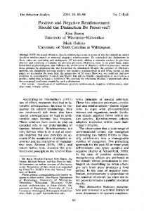
Fig. 1. Examples of Positive equivalence constraints (PECs – creatures paired by light-gray frames) and Negative equivalence constraints (NECs – creatures paired by dark-gray frames) using ”alien creatures” created for the cognitive experiments. Note that no labels were used for specifying the categorical relations between creatures. In the current example, the pre-selected task-relevant dimensions are skin color and ear shape: (a) Two pairs showing one randomly selected PEC (left the two creatures are from the same category despite differences in eye color and nose shape, since they share similar properties in the relevant dimensions) and one NEC (right, the two creatures differ in skin color, but also in some non relevant dimensions such as eye color and nose/chin shape). (b) Two pairs of highly informative constraints in which each pair differs in only one dimension, which is irrelevant in the case of PECs (left, eye color) and relevant in the case of NECs (right, face color).

The importance of investigating the separate contributions of PECs and NECs lies in the different ways that they are used and in their different basic properties. Though it would seem that the two types are equally important for category learning, actually they have very different characteristics, deriving both from how prevalent and how informative they are. The most obvious and intuitive underlying difference is that PECs may be compactly represented and efficiently satisfied, while simultaneous satisfaction of NECs is computationally difficult, usually requiring application of an approximation scheme. In Section 2 we measure the differential use of PECs and NECs by humans. Our results suggest that people use PECs quite intuitively, but demonstrate a common difficulty in using the naturally less informative NECs. Even when we set up an experiment whereby NECs and PECs provide the same amount of information, many

266

R. Hammer et al.

participants fail to use NECs efficiently. On the other hand, providing them with directions for the use of NECs dramatically improves performance, whereas the efficacy of using PECs is unchanged by the provision of similar directions. For further details concerning the experimental design and human findings reviewed here, see [9]. To gain further insight into the separate use of PECs and NECs, in Section 3 we analyze their separate contributions when incorporated into a clustering algorithm, using the constrained-EM algorithm suggested by Shental et al. [14]. The latter is an extension of the Expectation Maximization (EM) algorithm for estimating a Gaussian Mixture Model (GMM), which can make use of equivalence constraints of either type. While the constrained EM algorithm has been applied previously to several realworld datasets and shown to significantly enhance performance compared to its unconstrained counterpart [14], here we test this algorithm in a scenario which simulates the human experiments described above. We stress that the computer experiments should not be considered as direct simulations of the cerebral events underlying the behavioral results. However, as shown below, comparison of the two results leads to interesting observations regarding the possible use of PECs and NECs. Specifically, the results of the computer experiments may have similar properties to human performance – stemming from the fact that they both perform classifications in the same context, using similar information. These shared properties may be understood more easily from the computer experiments, and hopefully can be used to improve our understanding of human performance characteristics. In Section 4 we provide a formal basis for the computational difference between the use of PECs and NECs. Our analysis involves two distinct and complementary arguments: First of all, in Section 4.1 we use the language of complexity theory to argue that satisfying positive constraints can be done efficiently, while satisfying negative constraints is essentially intractable. Secondly, in Section 4.2 we define a measure of information for both types of constraints, and show that PEC information content is typically much larger than that of NECs.

2 Experiments and Results in Human Category Learning In order to investigate how people use PECs and NECs, we conducted three categorylearning experiments in which the two types of constraints were presented separately. In each experiment, participants performed a simple rule-based categorization of novel stimuli ("alien creatures faces'') in which the relevant or irrelevant dimensions had to be identified by either the PECs or NECs provided. In each trial, participants reviewed three constrained object pairs and were then asked to identify which objects belong to the same category as a given standard. Thus, participants needed to learn from the constraints which dimensions are relevant for the current trial, and to compare the trial standard with the other objects solely on the basis of these dimensions. Note that in many trials the constrained objects belonged to different categories than that of the standard provided. In each experimental condition, participants performed 10 trials. Performance level is presented using the nonparametric sensitivity measure A' defined as

Classification with Positive and Negative Equivalence Constraints

267

⎡ ( H − F )2 + | H − F | ⎤ A' = 0.5 + ⎢sign( H − F ) × ⎥ 4 × max(H , F ) − 4 × H × F ⎦ ⎣

where H represents the normalized Hits and F represents the normalized FalseAlarms. Score of 0.5 represents poor performance and score of 1 represents perfect performance. For further information concerning non-parametric signal analysis measures, see [8, 15]. 2.1 Experiment 1: Randomly Selected Constraints In order to evaluate the expected contribution of the two types of constraints in natural scenarios, when there is no deliberate selection of constraints to maximize the information provided to the classifier, in the first experiment we compared performance when using randomly selected PECs or NECs (see example in Fig. 1a) with a control condition where no equivalence constraints are provided (the "noEC" condition). The random constraints were preselected at the design stage (all participants were faced with the same constraints). Paired sample t-tests (see also Figure 2 left) showed that participants’ performance with a random set of three PECs was better than with either three random NECs, t(11) = 4.81, p < 0.001, d = 2.90, or with no constraints at all, t(11) = 4.33, p < 0.005, d = 2.61. There was no significant difference between performance in the random NEC and noEC conditions t(11) = 1.02, p = 0.33.

Fig. 2. Mean A′ scores with standard errors in all conditions. Exp 1: 12 participants, within-subject design: random PECs (0.83 ± 0.02), random NECs (0.75 ± 0.02), and no constraints (0.73 ± 0.01). Exp 2: 80 participants, between-subject design: highly informative highPECs (0.85±0.07) and highNECs (0.83 ± 0.13). Exp 3: 12 participants, within subject design: directed PECs (0.88 ± 0.07) and NECs (0.95 ± 0.04).

2.2 Experiment 2: Highly Informative Sets of Constraints The results of Experiment 1 can simply derive from the fact that a small random set of PECs provide more information than a small random set of NECs, and not necessarily from the fact that classifying with NECs is more complex than with PECs (as will be shown in section 4). Thus, this result probably reflects inherent properties of the constraints and not participant proficiency in their use. Experiment 2 therefore tested

268

R. Hammer et al.

the use of PECs and NECs when these were specifically chosen to provide all the information needed for perfect performance. Figure 1.b presents an example of such highly informative PECs and NECs. Importantly, we found a difference here, too, in performance with PECs vs. NECs. Although independent sample t-test showed that the mean level of performance with highPECs was not different from that with highNECs, t(78) = 0.85 (see Fig. 2 middle), the Leven test for homogeneity of variances showed that the standarddeviation in the highPEC condition was significantly smaller than in the highNEC condition, F(78) = 13.94, p < 0.001. The Shapiro-Wilk test of normality further showed that although in the highPEC condition, sensitivity was normally distributed, W(40) = 0.95, p = 0.11, the sensitivity distribution in the highNEC condition differed significantly from normal, W(40) = 0.89, p < 0.001. Interestingly, we found that participants may be divided into two groups: those who are able to use informative NECs quite well (with above-median Hit and below-median FA rates in Fig. 3, right inset), and those who are unable to do so (with below-median Hit and above-median FA rates). This raises the possibility that using NECs is not only computationally difficult, but that it may be non-intuitive for some participants to derive the proper strategy for their use, perhaps due to their inexperience with informative NECs in most natural settings.

Fig. 3. Histograms of sensitivity showing its distribution across participants with highPECs (left) and highNECs (right). Dashed curves represent the expected normal distribution given the observed mean and standard deviation. Boxes represent the corresponding ROC (Receiver Operating Characteristic) diagrams, where dashed lines represent each group median FA (Vertical) and median Hit (horizontal).

2.3 Experiment 3: Highly Informative Constraints with Directions Having found in Experiment 2 that some participants have difficulty using even informative NECs, we provided all participants in Experiment 3 with directions for the use of either highPECs or highNECs (identical to the constraints used in Exp. 2). We found that when provided with these directions all participants succeeded in using either type of constraint. Moreover, the bimodal pattern of performance with highNECs observed in Experiment 2 was replaced by a uniformly high success rate,

Classification with Positive and Negative Equivalence Constraints

269

and performance was higher than in the directed-highPEC condition, t(11) = 3.29, p < 0.01, d = 1.98; see Fig. 2 right. These findings further support the interpretation that it is the difference between PECs and NECs in natural circumstances that leads to the different proficiencies in their use. 2.4 Summary and Discussion Evaluating baseline performance with randomly selected constraints in Experiment 1, we found a clear advantage for category learning from PECs compared to NECs. Moreover, random NECs were poorly informative, leading to categorization performance similar to that observed when participants merely performed associative categorization (in the control condition without constraints). Experiment 2 demonstrated that deliberately selected PECs, containing all the information needed for perfect performance, are in fact not more informative than randomly selected PECs. In contrast, informative NECs enabled much better performance than randomly selected NECs at least for some participants. Taken as a group, participants in the highPEC and highNEC conditions had similar performance. However, further analysis revealed that in the highNEC condition, the performance distribution was bimodal with a relatively large standard-deviation. This highNEC condition bimodality was also apparent in the Hit and False-Alarm distributions, with about half of the participants in the highNEC condition performing almost perfectly and the other half performing very poorly, as though they had not received any informative constraints at all. In contrast, in the highPEC condition, performance was quite good for all participants, reaching only rarely the extremes of nearly-perfect or very poor performance.

Fig. 4. Schematic summary of performance in the three experiments described above – with randomly chosen constraints (I) or highly informative constraints, without (II) or with (III) directions for their use

Providing directions for the use of the constraints in Experiment 3 revealed a number of surprising results. First of all, we found that the strategy for using highNECs could be readily learned via simple instructions, leading participants to nearly perfect performance. This result suggests that the failure of the poor

270

R. Hammer et al.

performance subgroup in using highNECs was due to their inability to find the correct strategy, and not an inability to adopt new strategies. Still, it is surprising that a strategy for using highNECs was easily learned when instructions were provided, but many people (university students!) failed in intuitively implementing this strategy when performing the task without instruction. Secondly, we found that giving similar instructions for the best strategy for using PECs did not improve performance and participants remained at quite good, but not perfect performance levels. These differences between the benefit of instructions for using PECs and NECs were rather unexpected, and support our main claim that people use PECs, but not NECs, intuitively. Figure 4 summarizes participant performance in the three experiments.

3 Experiments Using the Constrained-EM Algorithm In this section we analyze the contribution of PECs and NECs when separately incorporated into the constrained-EM clustering algorithm [14]. Recently, equivalence constraints have been used for learning distance functions and for clustering [2, 3, 10, 17]. A number of clustering algorithms have been adapted to incorporate equivalence constraints, including K-means [16], complete-linkage [12] and an EM of a Gaussian Mixture Model (GMM) [14]. While most of these algorithms can easily incorporate positive constraints, incorporating negative constraints into these algorithms is usually much harder computationally and requires the application of various heuristics, or approximations. 3.1 Experimental Setup Our experiments were designed to replicate the experimental setup described above: Each of the 32 different alien faces was represented by a binary 5-dimensional vector. The constraint information provided to the algorithm was identical to that presented to human participants. As in the cognitive experiments, we ran the constrained EM algorithm in the randEC and highEC conditions, comparing each to the baseline noEC condition. Also, the test stage consisted of evaluating the quality of the cluster associated with the given standard, which was selected at random. Performance was measured using the A' score, defined above. Each “subject” was simulated using 5 different realizations of PECs and NECs, for which we averaged the A' scores, as done in our cognitive experiments. The EM algorithm is a gradient-based method which converges to a local maximum of the data likelihood. The algorithm is therefore very sensitive to its initial conditions, which implicitly determine the local maximum to which the algorithm will converge. Our results were therefore averaged over 200 different “subjects”, each performed five different categorization tasks. 3.2 Experimental Results Figure 5 displays performance (A') histograms for the constrained EM algorithm when trained using NECs and PECs, respectively. Results for the 2 conditions (averages and standard deviations) are also summarized in Table 1.

Classification with Positive and Negative Equivalence Constraints

271

Based on the results reported in Shental et al. [14], in which the constrained EM algorithm was tested on real world datasets, it came as no surprise to see that (on average) the constrained EM which used PECs achieved better A' scores than the same algorithm using only NECs. This is the case with both the random and the informative sets of constraints. There is no significant difference between performance using PECs in the two conditions, and no significant difference between average performance without constraints (noECs) compared to using NECs. This is in agreement with the human psychophysical findings above. When highNECs are provided, average performance is significantly higher than in the noEC condition, but still significantly lower than with highPECs. Unlike the results with human participants, the distribution of the highNEC scores is unimodal. This may suggest that the constrained-EM does not make optimal use of highNECs, similar to the "poorly-performing" human participants.

Fig. 5. Histograms of A′ scores of the GMM simulations using the constrained EM algorithm. Left: Results of the random equivalence constraints (randEC) condition. Right: Results of the highly informative constraints (highEC) condition.

Performance in the unsupervised noEC condition is above chance similar to our findings in the cognitive experiments. This is due to use of proximity relations which rule out many impossible groupings. As in our cognitive experiments, performance in the randNEC condition is not significantly better than in the noEC condition, since these constraints are usually non-informative. However, when informative constraints are provided, the algorithm seeks a solution which also complies with the constraints, and this additional information can, in many cases, direct the algorithm towards better solutions both in terms of refining the cluster centers (easily done with PECs) and the deviation from the cluster centers (NECs and PECs). Table 1. Average sensitivity scores of the constrained EM algorithm for the noEC, randEC and highEC conditions

Condition: randEC highEC

noEC 0.77 ± 0.04 0.77 ± 0.04

NECs 0.78 ± 0.04 0.85 ± 0.04

PECs 0.97 ± 0.02 0.99 ± 0.01

272

R. Hammer et al.

4 The Underlying Difference Between PECs and NECs In order to provide a formal basis for the computational difference between negative and positive constraints, we analyze the problem in two ways. First, in Section 4.1 we show that clustering with NECs is related to the problem of finding the maximal cut in a graph, which is known to be very hard (NP-complete). In contrast, clustering with PECs is related to the analogous problem of finding the minimal cut in a graph, for which efficient polynomial algorithms are known. Secondly, in Section 4.2 we define the notion of information for both types of constraints, and obtain a lower bound on the difference in information content between positive and negative constraints. Specifically, the information content of NECs is inversely related to the number of different graph colorings for the graph defined by the negative constraints. Computing this number is very hard (again, an NP-hard problem), with no known approximations [11]. More importantly, for random graphs it is known that the number of solutions tends to be very large whenever there is a solution to the coloring problem. In contrast, the number of colorings for a graph defined by positive constraints is rather small due to transitivity. Thus, the difference in information content between PECs and NECs is typically very large. Notation We represent the data as a graph G = {V,E}, where the set of nodes V of size N corresponds to the datapoints, and the set of edges E of size M corresponds to the given constraints, either positive or negative (but not both). The task is to divide the data-points into K classes. 4.1 The Complexity of Satisfying Positive or Negative Constraints Assume K = 2, and the task is therefore to partition the data into two clusters. Each partition is represented by C – the set of all edges from E which connect nodes assigned to different clusters; the set C is called the cut of graph G. Each cut is assigned a cost – the number of edges in C. Enforcing positive constraints is manageable Given positive constraints, we seek a partition in which as few positive constraints as possible are violated. Finding this partition is equivalent to finding the minimal cut in the above graph. There are known efficient algorithms to solve this problem. Thus, in the complexity hierarchy of computer science, this problem is considered tractable. Enforcing negative constraints is hard Given negative constraints, we seek a partition in which as few negative constraints as possible are violated. Finding this partition is equivalent to finding the maximal cut in the graph defined above. There are no known efficient algorithms to solve this problem. Therefore, in the complexity hierarchy of computer science, this problem is almost certainly intractable.

Classification with Positive and Negative Equivalence Constraints

273

4.2 The Information Content of Positive or Negative Constraints We define the information of a set of constraints E to be the difference between the entropy H of all the partitions of the set of nodes V to K clusters,1 and the entropy HG of all such partitions consistent with E. Assuming that each allowed partition is assigned equal probability, the entropy HG is equal to the log of the number of allowed partitions. We are interested in the difference between the information of positive and negative constraints, namely in

I = ( H − H G+ ) − ( H − H G− ) = H G− − H G+ = log

#G− #G+

(1)

where the entropy superscript + or – denotes respectively whether the set of constraints is positive or negative,

#G− denotes the number of partitions consistent

with E if the constraints are negative, and

#G+ is similarly defined if the constraints

are positive. To compute

#G+ we note that all the nodes in every connected component of the

graph G should be assigned to the same cluster in each allowed partition2. We can therefore treat every connected component as a single meta-node, and the number of different partitions is

#G+ = K N c

(2)

where NC denotes the number of connected components of G. In particular, if the graph G has no loops, NC = N – M and therefore

#G+ = K N − M

(3)

where M is the number of edges in E. It is quite hard to compute

#G− in the general case: it represents the different

number of colorings of graph G, a number whose computation is known to be NPhard. We start with the simple case where graph G has no loops, for which we can show that

#G− = K N − M ( K − 1) M

(4)

This result can be readily proven by induction on the number of constraints M. We can now state the first result of this section: Result 4.1 When the graph of constraints has no loops, as in the experiments described above, the information gain of positive over negative constraints is 1

We allow partitions that assign no node to one or more clusters. However, it can be readily shown that the number of such partitions is negligible when N >> K. 2 A connected component is a subset of nodes that are connected to each other by edges from E.

274

R. Hammer et al.

I = M log( K − 1) The result follows from substituting (3) and (4) into (1). For a general graph with NC connected components, we note that each connected component in G has at least one legal coloring (by assumption). We immediately get the following bound NC

# ≥∏ − G

i =1

K l K! = ∏ ( K − l + 1) N C ( K − qi )! l =1

(5)

where qi denotes the number of nodes in the i-th connected component (if smaller l

than K, or K otherwise), and N C denotes the number of connected component with l or more elements N C = N C1 ≥ N C2 ≥ ... ≥ N CK . Substituting (5) and (2) into (1) we get the second result: Result 4.2 The information gain of positive over negative constraints satisfies K

I ≥ ∑ N Cl log( K − l + 1) l =2

This bound is rather loose, as it is derived by assuming that each connected component has only one coloring solution. Typically, however, the situation is quite different: if a graph has any solution at all, it would typically (for random graphs) have an exponential number of solutions (Krivelevich, 2002). We can therefore state that, If N >> NC, the information content of positive constraints is exponentially larger than negative constraints.

5 Discussion We investigated properties of PECs and NECs and their effects on performance in a classification task – in the context of human cognition and machine learning. Parallel theoretical analyses demonstrated that the use of NECs is computationally much more difficult than use of PECs, and that NECs convey less information than do PECs. In accordance with this theoretical result, our cognitive experiments found that humans can easily make use of randomly-chosen PECs, but random NECs do not provide any gain in performance compared to the no-constraints baseline condition. Computer experiments similarly found improved performance only with random PECs. While the EM algorithm does not necessarily simulate human categorization strategies, it does demonstrate that the difficulties in using NECs are inherent. The theoretical analysis implies that our results are general and not limited to the rule-based classification task (that assumes an object space whose dimensionality may be

Classification with Positive and Negative Equivalence Constraints

275

reduced in a consistent manner) or the EM algorithm (that assumes a Euclidean object space with proximity representing similarity). If the limitation in using NECs derives from their properties when chosen at random, informative NECs should allow good performance. Surprisingly, we discovered that only about half of the participants succeeded in properly using highly informative NECs, selected to pinpoint a single relevant dimension. Our computer experiments found an improvement with highNECs, but not to the level achieved by highPECs. These results may derive from the good performing participants shifting their classification strategy, while the poor performers were unable to do so. The computer algorithm, also unable to change its strategy, similarly obtained only moderate improvement. The poor performance by many human participants is consistent with the hypothesis that since NECs are generally less informative than PECs, people lack experience in their use and many fail to use them even when they are informative. This hypothesis is supported by the finding that the provision of directions allowed all participants to achieve very good performance with highPECs. If people are generally not experienced in the use of NECs for general classification scenarios, are NECs useful at all? One possibility is that NECs are important for the difficult task of identifying fine, yet important differences between highly similar categories – as in subordinate-level categories or perceptual learning requiring identification of subtle differences between stimuli. In these cases, informative NECs may increase the perceived dissimilarities [7] leading to refinement of the classifier conceptual knowledge.

References [1] Ashby, F.G., Maddox, W.T.: Human category learning. Ann. Rev Psychology 56, 149– 178 (2005) [2] Bar-Hilel, A., Hertz, T., Shental, N., Weinshall, D.: Learning distance functions using equivalence relations. In: The 20th International Conference on Machine Learning (2003) [3] Bilenko, M., Basu, S., Mooney, R.J.: Integrating constraints and metric learning in semisupervised clustering. In: Banff Canada, AAAI press, Stanford, California, USA (2004) [4] Bishop, C.M.: Neural Networks for Pattern Recognition. Oxford press, Oxford (1995) [5] Cohen, A.L., Nosofsky, R.M.: An exemplar-retrieval model of speeded same-different judgments. Journal of Experimental Psychology: Human Perception and Performance 26, 1549–1569 (2000) [6] Duda, R.O., Hart, P.E., Stork, D.G.: Pattern Classification. John Wiley and Sons Inc., Chichester (2001) [7] Goldstone, R.L.: Influences of categorization on perceptual discrimination. Journal of Experimental Psychology: General 123(2), 178–200 (1994) [8] Grier, J.B.: Nonparametric indexes for sensetivity and bias: Computing formulas. Psychological Bulletin 75, 424–429 (1971) [9] Hammer, R., Hertz, T., Hochstein, S., Weinshall, D.: Category learning from equivalence constraints. Cognitive Processing (in press) [10] Hertz, T., Bar-Hillel, A., Weinshall, D.: Boosting margin based distance functions for clustering. In: ICML (2004)

276

R. Hammer et al.

[11] Khanna, S., Linial, N., Safra, S.: On the hardness of approximating the chromatic number. Combinatorica 1(3), 393–415 (2000) [12] Klein, D., Kamvar, S., Manning, C.: From instance-level constraints to space-level constraints: Making the most of prior knowledge in data clustering. In: Proceedings of the Nineteenth International Conference on Machine Learning (2002) [13] Krivelevich, M.: Sparse graphs usually have exponentially many optimal colorings. Electronic Journal of Combinatorics 9 (2002) [14] Shental, N., Bar-Hilel, A., Hertz, T., Weinshall, D.: Computing Gaussian mixture models with EM using equivalence constraints. In: Advances in Neural Information Processing Systems, vol. 16, MIT Press, Cambridge (2004) [15] Stanislaw, H., Todorov, N.: Calculating signal detection theory measures. Behavior Research Methods, Instruments, & Computers 31(1), 137–149 (1999) [16] Wagstaff, K., Cardie, C., Rogers, S., Schroedl, S.: Constrained K-means clustering with background knowledge. In: Proc. 18th International Conf. on Machine Learning, pp. 577–584. Morgan Kaufmann, San Francisco, CA (2001) [17] Xing, E.P., Ng, A.Y., Jordan, M.I., Russell, S.: Distance metric learnign with application to clustering with side-information. In: Advances in Neural Information Processing Systems, vol. 15, MIT Press, Cambridge (2002)