arXiv:1506.00815v3 [cs.CV] 6 Jun 2015
Classify Images with Conceptor Network
Ishwarya M S Advanced Robotic Lab Department of Artificial Intelligence Faculty of Computer Science & IT University of Malaya
[email protected]
Yuhuang Hu Advanced Robotic Lab Department of Artificial Intelligence Faculty of Computer Science & IT University of Malaya
[email protected]
Chu Kiong Loo Advanced Robotic Lab Department of Artificial Intelligence Faculty of Computer Science & IT University of Malaya
[email protected]
Abstract This article demonstrates a new conceptor network based classifier in classifying images. Mathematical descriptions and analysis are presented. Various tests are experimented using three benchmark datasets: MNIST, CIFAR-10 and CIFAR100. The experiments displayed that conceptor network can offer superior results and flexible configurations than conventional classifiers such as Softmax Regression and Support Vector Machine (SVM).
1 Introduction Recent successes in deep learning has revolutionized the field of machine learning and pattern recognition [1, 2, 3, 4, 5, 6, 7]. In most successful classification applications, softmax regression [8] and support vector machine (SVM) [9] are usually employed and achieved state-of-the-art performance [2, 3, 7]. One major disadvantage of current popular classifiers (i.e. softmax regression) is that they are not extensible once the learning architecture is built. In a supervised learning task, current classifiers are not capable of modeling new class of data by default. They have to reinitialize the entire architecture or pay expensive cost on retraining the learning model. Another disadvantage of current classifiers is that they fail to model logical relationships in between classes. This usually prevents us from conducting semantic reasoning directly using non-semantic information (i.e. image feature, audio feature). This article utilized a naive conceptor network [10] as classifier for image classification benchmarks (details in Section 2). The network generates a conceptor for each presented class. As the name suggested, a conceptor represents the “concept” of a class. And then learned conceptors are used to measure relevance between data and the classes. Three popular datasets: MNIST [11], CIFAR10 [12] and CIFAR-100 [12] are experimented and analyzed (Section 3). The experiments showed that conceptor network is capable of achieving comparable performance on MNIST (97.49%) and superior performance on CIFAR-10 (98.39%) and CIFAR-100 (83.04%) datasets using simple features from shallow neural networks (Section 3.1–3.3). The model is capable of learning new unseen classes without damaging the performance of previous learned classes (Section 3.4). In the addition experiment of CIFAR-100, the learned sub-class conceptors can infer super-class conceptors without retraining by using logical operations (Section 3.5). 1
2 Method 2.1 Naive conceptor network Consider a modified recurrent network: ht = σ(Whh ht−1 + Wih xt + b) (1) y t = ht (2) where σ(·) is the activation function (tanh in this article). xt ∈ Rn is an n-dimensional input at time t. ht ∈ Rm is an m-dimensional hidden activation at t, the output of the network yt is a replica of hidden activation. Whh and Wih are weight matrices from hidden to hidden and from input to hidden correspondingly. Note that all weight matrices are initialized randomly and not subjected to change over time. Let X = {xt }t=T t=1 is a time-dependent pattern or a class of data (i.e. object, face, scene, etc) and m×T H = [ht ]t=T (h0 is randomly initialized) as respective hidden activation history. The t=1 ∈ R hidden activation can be modeled by following cost function:
J(H, C, λ) =
T 1 X ||ht − Cht ||2 + λ||C||2fro T t=1
(3)
where C is called conceptor that characterizes data X’s hidden activation H, λ ∈ (0, 1) is the regularization term. Given Eqn. 3, conceptor C can be computed by empolying stochastic gradient descent (SGD) by ∂ J (4) C′ = C + α ∂C where α is learning rate. Since Eqn. 3 presents a convex problem, there is an analytical solution given by [10, 13]: C = R(R + λI)−1 m×m where R ∈ R is correlation matrix that is computed by HH ⊤ R= T
(5) (6)
Eqn. 4 and Eqn. 5 are expected to give the same solution under regularization. Considering the speed issue and size of datasets that are used in this paper, the analytical solution is primarily used. Correlation matrix R characterizes geometrical properties of hidden activation. By running principal m component analysis (PCA), the resulted eigenvectors v = {vi }m i=1 and eigenvalues Σ = {σi }i=1 represent an ellipsoid in high dimensional space. Eqn. 3 is subject to learn a regularized identity map. One perspective of conceptor C is a normalized version of R, the eigenvalues σi are normalized to ci is: σi ci = (7) σi + λ The above equation normalizes the eigenvalues into (0,1). ci s here are eigenvalues of conceptor C. C preserve the geometrical properties still. 2.2 Use logical operations over conceptor An advantage that is offered by conceptor network is enabling boolean operations [10]. Basic boolean operations such as NOT (¬), AND (∧), OR (∨) are usable over learned conceptors. Given conceptors B, C and identity matrix I, operations that are suggested in [10] are listed here: • NOT • AND
¬C = I − C
(8)
C ∧ B = (C −1 + B −1 − I)−1
(9)
C ∨ B = ¬(¬C ∧ ¬B)
(10)
• OR
2
2.3 Use conceptor network as supervised classifier Conceptor network takes a regression analysis on hidden activation of a class of data. The resulted conceptor has the property of quantifying relevance between a hidden activation using vector projection (Section 2.1). This advantage can be taken to formulate a supervised classifier. Let C = {Cj }N j=1 as a collection of conceptors. Each conceptor Cj characterizes one class of data. Let D = {Dj }N j=1 as a collection of negative conceptors that produced by C: Dj = ¬(C1 ∨ C2 ∨ . . . ∨ Cj−1 ∨ Cj+1 ∨ . . . ∨ CN )
(11)
where Dj represents the condition of not being other N − 1 classes. Given a conceptor C, a negative conceptor D and data x’s hidden activation h, a positive evidence is computed by E + (C, h) = h⊤ Ch (12) Correspondingly, negative evidence is E − (D, h) = h⊤ Dh
(13)
And combined evidence is computed by E(C, D, h) = E + (C, h) + E − (D, h)
(14)
Positive evidence quantify the degree of relevance between signal x and conceptor C. Negative evidence quantify the degree of relevance between signal x and not being other classes than C. The evidence computes overlapping between the ellipsoids that is characterized by conceptor C and the data. Given data x’s hidden activation h, the signal belongs to class j ∗ : j ∗ = arg max E(Cj , Dj , h) j = 1, . . . , N j
(15)
where Cj ∈ C and Dj ∈ D.
3 Experiments In this section, experiments on MNIST, CIFAR-10 and CIFAR-100 are presented and discussed. All images are rescaled in [0, 1]. Images in CIFAR-10 and CIFAR-100 are converted in gray-scale. No further pre-processing is performed. Image features are extracted from either a one-hidden-layer auto-encoder/a Convolutional Neural Network (ConvNet). ConvNet in this article has two convolution layers, one fully connected layer and one softmax layer, features are extracted from the fully connected layer. ConvNet is employed here to produce better image features than auto-encoder. The naming method of feature is [AE/ConvNet]-Feature-[Dimension of each feature] (e.g. AE-Feature-200 represents a set of autoencoder features with 200 dimensions). Conceptor network directly takes features of images for classification. There are 3 types of experiments are performed for each dataset: 1. Classification performance V.S. Number of hidden neurons 2. Classification performance V.S. Input feature size 3. Classification performance V.S. Feature extraction method (AE feature/ConvNet feature) And 2 additional experiments are performed in order to test logical operations: 1. Learning new class without damaging previous learned classes (CIFAR-100 sub-classes). 2. Infer super-class conceptors from sub-class conceptors (CIFAR-100) 3
3.1 Classify MNIST MNIST dataset contains 60,000 training samples and 10,000 testing samples [11]. Each sample is a hand-written digit from 0-9. Experiments in this section used first 50,000 samples of training dataset and full testing dataset. The conceptor network generated 10 conceptors for total 10 classes given a set of feature. Results are presented in Figure 1 and Tab. 1. In Fig. 1, performance of conceptor network is stable across a large range of number of neurons in reservoir. And the network works well when the number of neurons is small. Results in Tab. 1 shows that Auto-encoder feature is slightly better than ConvNet feature. The performance here is not as good as some deep architectures [11, 14]. It offered similar performance to networks that have similar depth (3 layer MLP networks used in [11]).
Classification accuracy (%)
100
AE Feature 200
ConvNet Feature 200
AE Feature 500
ConvNet Feature 500
90 80 70 60 50 0
50
100
150 200 250 300 350 Number of hidden neurons
400
450
500
Figure 1: MNIST Classification Results
Table 1: MNIST Classification Results & Comparison Feature Type Number of Accuracy hidden neurons AE-Feature-200 125 96.85% ConvNet-Feature-200 20 95.77% AE-Feature-500 10 97.49% ConvNet-Feature-500 10 95.93% Method Accuracy Y. Lecun et al. [11] 99.05% R. Salakhutdinov et al. [14] 99% Y. Lecun et al. [11] 97.05%
3.2 Classify CIFAR-10 CIFAR-10 consists of 60,000 32 × 32 color images in 10 classes [12]. There are 50,000 training images and 10,000 testing images. CIFAR-10 is among the most popular benchmarks in pattern recognition. Like MNIST, experiments here also employ features from shallow networks. And results are showed in Fig. 2 and Tab. 2. ConvNet features are performing better than Auto-encoder features in these experiments (Tab. 2). The best result is produced by ConvNet-Feature-500 with accuracy of 98.39%. Classification results presented here have reached or been better than state-of-the-art methods [15, 16, 17, 18] (Tab. 2). 4
Classification accuracy (%)
100
AE Feature 200
ConvNet Feature 200
AE Feature 500
ConvNet Feature 500
90 80 70 60 50 0
50
100
150 200 250 300 350 Number of hidden neurons
400
450
500
Figure 2: CIFAR10 Classification Results
Table 2: CIFAR-10 Results Feature Type Number of hidden neurons AE-Feature-200 5 ConvNet-Feature-200 5 AE-Feature-500 490 ConvNet-Feature-500 100 Method C.-Y.Lee et al. [15] M.Lin et al. [16] L. Wan et al. [17] I. J. Goodfellow et al. [18]
Accuracy 85.04% 98.30% 88.09% 98.39% Accuracy 91.78% 91.2% 90.68% 90.65%
3.3 Classify CIFAR-100 CIFAR-100 consists of 60,000 32 × 32 color images in 100 classes [12]. Each class has 500 training images and 100 testing images. And the 100 classes are grouped into 20 super-classes. There are many previous attempts on improving classification accuracy for CIFAR-100 [15, 16, 18, 19]. The results are presented in Figure 3, 4 and Table 3, 4. Similar to previous results in CIFAR-10, ConvNet features in this section work a lot better than Auto-encoder features (10%-20% better in CIFAR-100 sub-class experiment). Both best results of super-class and sub-class classification are generated by ConvNet-Feature-500 (96.48% and 83.04% respectively). Performance of proposed method is better than previous published results (Tab. 4).
Table 3: CIFAR-100 Super-classes Results Feature Type Number of Accuracy hidden neurons AE-Feature-200 365 87.67% ConvNet-Feature-200 5 94.81% AE-Feature-500 10 88.99% ConvNet-Feature-500 20 96.48%
5
Classification accuracy (%)
100
AE Feature 200
ConvNet Feature 200
AE Feature 500
ConvNet Feature 500
90 80 70 60 50 0
50
100
150 200 250 300 350 Number of hidden neurons
400
450
500
Figure 3: CIFIR 100 Super-classes Classification Results
Classification accuracy (%)
100
AE Feature 200
ConvNet Feature 200
AE Feature 500
ConvNet Feature 500
90 80 70 60 50 0
50
100
150 200 250 300 350 Number of hidden neurons
400
450
500
Figure 4: CIFAR-100 Sub-classes Classification Results Table 4: CIFAR-100 Sub-classes results Feature Type Number of Accuracy hidden neurons AE-Feature-200 10 65.28% ConvNet-Feature-200 10 76.59% AE-Feature-500 25 62.96% ConvNet-Feature-500 20 83.04% Method Accuracy C.-Y.Lee et al. [15] 65.43% M.Lin et al. [16] 64.32% N. Srivastava et al. [19] 63.15% I. J. Goodfellow et al. [18] 61.43%
3.4 Learn new classes incrementally Another advantage of conceptor network is that it can learn new classes without damaging previous learned classes. With this feature, a learning system can be easily scaled up without taking many efforts. This experiment takes 100 sub-classes of CIFAR-100 to demonstrate incremental learning. 6
ConvNet Feature 200
Classification accuracy (%)
100
ConvNet Feature 500
80 60 40 20 0 2
9
16 23 30 37 44 51 58 65 Number of classes
72 79 86 93 100
Figure 5: CIFAR-100 Super-classes Incremental Learning Results The network is initially trained with 2 of all 100 classes. Then a conceptor is computed when the network observed a new class. The new conceptor is then appended in the list of existed conceptors. And it can be used to classify new data along with old ones. Fig. 5 presents the result of the experiment. The network in this experiment consists of 180 hidden neurons. The blue line is the result generated by ConvNet-Feature-200 (average accuracy: 77.55%) and the red line is the result generated by ConvNet-Feature-500 (average accuracy: 83.81%). Both results are stable during learning new classes incrementally. 3.5 Infer super-classes from sub-classes in CIFAR-100 One feature of CIFAR-100 is relationship between super-class and sub-class. As discussed previously, each super-class corresponds to 5 sub-classes. Conventionally, a mapping table is used when a classifier (e.g. softmax) generates super-class label from sub-class label of an image.
Classification accuracy (%)
100
Sub-classes Feature 200
Sub-classes Feature 500
90 80 70 60 50 0
50
100
150 200 250 300 350 Number of hidden neurons
400
450
500
Figure 6: Classify CIFAR-100 Super-classes using Sub-classes Results In this experiment, logical operation OR is used to infer super-classes directly from sub-classes. For example, the conceptor of flowers can be represented as combination of it’s sub-classes orchids, poppies, roses, sunflowers and tulips: Cflowers = Corchids ∨ Cpoppies ∨ Croses ∨ Csunflowers ∨ Ctulips Here the conceptors established a semantic relationship between super and sub-classes instead of a simple mapping method. Concept of flowers is reasoned from its 5 sub-classes. One can use 7
this property of conceptor to model complex relationships between data categories. The result is presented in Fig. 6. The classification performance stays high and stable across large number range of hidden neurons.
4 Conclusion This article demonstrated our first attempt of using conceptor network in pattern recognition benchmarks. Conceptor network exhibited impressive performance on classification of tiny object images. The proposed classifier showed superior performance with shallow network features. It can learn new class of data incrementally without harming previous learned classes. And it is capable of modeling semantic relationships by using logical operations over learned conceptors. One challenge and problem is that this method takes high memory cost of maintaining all conceptors at once. This requirement is fair to most benchmark datasets, however it is not an ultimate solution for extreme large data flows. The potential of conceptor network is unlimited by current presentation. Our future works include exploring theory and applications of conceptor network. Many state-of-the-art supervised application now potentially can replace conventional classifiers with conceptor network. Acknowledgments This research is supported by High Impact Research UM.C/625/1/HIR/MOHE/FCSIT/10 from University of Malaya.
8
References [1] S. Ioffe and C. Szegedy, “Batch normalization: Accelerating deep network training by reducing internal covariate shift,” CoRR, vol. abs/1502.03167, February 2015. [2] J. Y.-H. Ng, M. Hausknecht, S. Vijayanarasimhan, O. Vinyals, R. Monga, and G. Toderici, “Beyond short snippets: Deep networks for video classification,” CoRR, vol. abs/1503.08909, March 2015. [3] A. Karpathy and L. Fei-Fei, “Deep visual-semantic alignments for generating image descriptions,” CoRR, vol. abs/1412.2306, 2014. [4] F. Schroff, D. Kalenichenko, and J. Philbin, “Facenet: A unified embedding for face recognition and clustering,” CoRR, vol. abs/1503.03832, Marchs 2015. [5] C. Szegedy, W. Liu, Y. Jia, P. Sermanet, S. Reed, D. Anguelov, D. Erhan, V. Vanhoucke, and A. Rabinovich, “Going deeper with convolutions,” CoRR, vol. abs/1409.4842, 2014. [6] V. Mnih, K. Kavukcuoglu, D. Silver, A. A. Rusu, J. Veness, M. G. Bellemare, A. Graves, M. Riedmiller, A. K. Fidjeland, G. Ostrovski, S. Petersen, C. Beattie, A. Sadik, I. Antonoglou, H. King, D. Kumaran, D. Wierstra, S. Legg, and D. Hassabis, “Human-level control through deep reinforcement learning,” Nature, vol. 518, no. 7540, pp. 529–533, February 2015. [7] A. Karpathy, G. Toderici, S. Shetty, T. Leung, R. Sukthankar, and L. Fei-Fei, “Large-scale video classification with convolutional neural networks,” in The IEEE Conference on Computer Vision and Pattern Recognition (CVPR), June 2014. [8] C. M. Bishop, Pattern Recognition and Machine Learning.
Springer, 2006.
[9] C.-C. Chang and C.-J. Lin, “Libsvm: A library for support vector machines,” ACM Trans. Intell. Syst. Technol., vol. 2, no. 3, pp. 27:1–27:27, 2011. [10] H. Jaeger, “Controlling recurrent neural networks by conceptors,” 2014. [11] Y. Lecun, L. Bottou, Y. Bengio, and P. Haffner, “Gradient-based learning applied to document recognition,” Proceedings of the IEEE, vol. 86, no. 11, pp. 2278–2324, Nov 1998. [12] A. Krizhevsky, “Learning multiple layers of features from tiny images,” 2009. [13] G.-B. Huang, H. Zhou, X. Ding, and R. Zhang, “Extreme learning machine for regression and multiclass classification,” Systems, Man, and Cybernetics, Part B: Cybernetics, IEEE Transactions on, vol. 42, no. 2, pp. 513–529, April 2012. [14] R. Salakhutdinov and G. Hinton, “Learning a nonlinear embedding by preserving class neighbourhood structure,” in Proceedings of the International Conference on Artificial Intelligence and Statistics, vol. 11, 2007. [15] C.-Y. Lee, S. Xie, P. Gallagher, Z. Zhang, and Z. Tu, “Deeply-supervised nets,” CoRR, vol. abs/1409.5185, 2014. [16] M. Lin, Q. Chen, and S. Yan, “Network in network,” CoRR, vol. abs/1312.4400, 2013. [17] L. Wan, M. D. Zeiler, S. Zhang, Y. LeCun, and R. Fergus, “Regularization of neural networks using dropconnect,” in Proceedings of the 30th International Conference on Machine Learning, ICML 2013, Atlanta, GA, USA, 16-21 June 2013, 2013, pp. 1058–1066. [18] I. J. Goodfellow, D. Warde-Farley, M. Mirza, A. C. Courville, and Y. Bengio, “Maxout networks,” in Proceedings of the 30th International Conference on Machine Learning, ICML 2013, Atlanta, GA, USA, 16-21 June 2013, 2013, pp. 1319–1327. [19] N. Srivastava and R. R. Salakhutdinov, “Discriminative transfer learning with tree-based priors,” in Advances in Neural Information Processing Systems 26, C. Burges, L. Bottou, M. Welling, Z. Ghahramani, and K. Weinberger, Eds. Curran Associates, Inc., 2013, pp. 2094–2102.
9