Apr 10, 2010 - The packing dimension is defined analogously and like Hausdorff dimension can be obtained as: dimP (E) = sup{s : hs â PE. â} = inf{s : hs â ...
arXiv:0905.1980v2 [math.CA] 10 Apr 2010
CLASSIFYING CANTOR SETS BY THEIR FRACTAL DIMENSIONS CARLOS A. CABRELLI, KATHRYN E. HARE, AND URSULA M. MOLTER Abstract. In this article we study Cantor sets defined by monotone sequences, in the sense of Besicovich and Taylor. We classify these Cantor sets in terms of their h-Hausdorff and h-Packing measures, for the family of dimension functions h, and characterize this classification in terms of the underlying sequences.
1. Introduction A natural way to classify compact subsets E ⊆ R of Lebesgue measure zero is by their Hausdorff or packing dimension. This is a crude measurement, however, which often does not distinguish salient features of the set. For a finer classification, one could consider the family of h-Hausdorff measures, H h , and h-packing measures, P h , where h belongs to the set of dimension functions D, defined in Section 2. Definition 1.1. By the dimension partition of a set E, we mean a partition of D E into (six) sets Hα ∩ PβE , for α ≤ β ∈ {0, 1, ∞}, where E Hα
H1E
= =
{h ∈ D : H h (E) = α} for α = 0, ∞, {h ∈ D : 0 < H h (E) < ∞},
and PβE is defined similarly, but with h-packing measure replacing h-Hausdorff measure. Sets which have the same dimension partition will have the same Hausdorff and packing dimensions, however the converse is not necessarily true. We call a compact, perfect, totally disconnected, measure zero subset of the real line a Cantor set. There is a natural way (see section 3.1) to associate to each summable, non-increasing sequence a = {an } ⊆ R+ , a unique Cantor set Ca having gaps with lengths corresponding to the terms an . The study of the dimension of Cantor sets by means of its gaps was initiated by Besicovich and Taylor [1]. In fact, the Hausdorff and packing dimensions of Ca can be calculated in terms of the tails P (a) of the sequence a, the numbers rn = i≥n ai , for n ∈ N. In this paper we show that the classification of the sets Ca according to their dimension partitions can be characterized in terms of properties of their tails. 2000 Mathematics Subject Classification. Primary 28A78, 28A80. Key words and phrases. Hausdorff dimension, Packing dimension, Cantor set, Cut-out set. C. Cabrelli and U. Molter are partially supported by Grants UBACyT X149 and X028 (UBA), PICT 2006-00177 (ANPCyT), and PIP 112-200801-00398 (CONICET). K. Hare is partially supported by NSERC. This paper is in final form and no version of it will be submitted for publication elsewhere. 1
2
C. CABRELLI, K.HARE, AND U. MOLTER
We introduce a partial ordering, �, on the set of dimension functions, which preserves the order of Hausdorff and packing h-measures. A set E is said to be h-regular if h ∈ H1E ∩ P1E . If this holds for h = xs then E is said to be s-regular, and in that case the Hausdorff and packing dimensions of E are both s. Although not every Cantor set, Ca , of dimension s is an s-regular set, we show that one can always find a dimension function h such that Ca is an h-regular set. This completes arguments begun in [2] and [5]. The dimension functions for which a given Cantor set, Ca , is regular form an equivalence class under this ordering and are called the dimension functions associated to the sequence a. We prove that two Cantor sets, Ca , Cb , have the same dimension partition if and only if their associated dimension functions, ha , hb , are equivalent. More generally, we prove that Ca and Cb have the same dimension partition if and only a and b are weak tail-equivalent (see Definition 4.2). Furthermore, we show that the weak tail-equivalence, can be replaced by the stronger tail-equivalence relation, only when the associated dimension functions have inverse with the doubling property. 2. Dimension Functions and Measures A function h is said to be increasing if h(x) < h(y) for x < y and doubling if there exists τ > 0 such that h(x) ≥ τ h(2x) for all x in the domain of h. We will say that a function h : (0, A] → (0, ∞], is a dimension function if it is continuous, increasing, doubling and h(x) → 0 as x → 0. We denote by D the set of dimension functions. A typical example of a dimension function is hs (x) = xs for some s > 0. Given any dimension function h, one can define the h-Hausdorff measure of a set E, H h (E), in the same manner as Hausdorff s-measure (see [6]): Let |B| denote the diameter of a set B. Then H h (E) = lim+ δ→0
�
inf
nX
h(|Ei |) :
[
Ei ⊆ E, |Ei | ≤ δ
o�
.
Hausdorff s-measure is the special case when h = hs . In terms of our notation, the Hausdorff dimension of E is given by E dimH E = sup{s : hs ∈ H∞ } = inf{s : hs ∈ H0E }.
The h-packing pre-measure is defined as in [7]. First, recall that a δ-packing of a given set E is a disjoint family of open balls centered at points of E with diameters less than δ. The h-packing pre-measure of E is defined by � nX o� h(|Bi |) : {Bi }i is a δ-packing of E . P0h (E) = lim sup δ→0+
It is clear from the definition that the set function P0h is monotone, but it is not a measure because it is not σ-sub-additive. The h-packing measure is obtained by a standard argument: ( ∞ ) X [ h h P (E) = inf P0 (Ei ) : E = Ei . i=1
The pre-packing dimension is the critical index given by the formula
dimP0 E = sup{s : P0hs (E) = ∞} = inf{s : P0hs (E) = 0}
CANTOR SETS
3
and is known to coincide with the upper box dimension [7]. Clearly, P h (E) ≤ P0h (E) and as h is a doubling function H h (E) ≤ P h (E) (see [8]). The packing dimension is defined analogously and like Hausdorff dimension can be obtained as: E } = inf{s : hs ∈ P0E }. dimP (E) = sup{s : hs ∈ P∞
Finally, we note that the set E is said to be h-regular if 0 < H h (E) ≤ P h (E) < ∞ and s-regular if it is hs -regular. The set, H1E ∩P1E , consists of the h-regular functions of E. We are interested in comparing different dimension functions. Definition 2.1. Suppose f, h : X → (0, A]. We will say f � h if there exists a positive constant c such that f (x) ≤ c h(x) for all x.
We will say f is equivalent to h, and write f ≡ h, if f � h and h � f . This defines a partial ordering that is consistent with the usual pointwise ordering of functions. It is not quite the same as the ordering defined in [5], but we find it to be more natural. Note that the definition of equivalence of functions, when applied to sequences, implies that x = {xn } and y = {yn } are equivalent if and only if there exist c1 , c2 > 0 such that c1 ≤ xn /yn ≤ c2 for all n. The following easy result is very useful and also motivates the definition of �. Proposition 2.2. Suppose h1 , h2 ∈ D and h1 � h2 . There is a positive constant c such that for any Borel set E, h2 h1 (E). (E) ≤ cP(0) H h1 (E) ≤ cH h2 (E) and P(0)
Proof. Suppose h1 (x) ≤ ch2 (x) for all x. For any δ > 0, nX o Hδh1 (E) = inf h1 (|Ui |), E ⊆ ∪i Ui , |Ui | < δ nX o ≤ c inf h2 (|Ui |), E ⊆ ∪i Ui , |Ui | < δ = cHδh2 (E).
The arguments are similar for packing pre-measure.
�
Corollary 2.3. If h1 , h2 ∈ D and h1 ≡ h2 , then for any Borel set E, h1 and h2 E belong to the same set Hα ∩ PβE . 3. Cantor sets associated to sequences 3.1. Cantor sets Ca . Each Cantor set is completely determined by its gaps, the bounded convex components of the complement of the set. To each summable sequence of positive numbers, a = {an }∞ n=1 , we can associate a unique Cantor set with gaps whose lengths correspond to thePterms of this sequence. ∞ To begin, let I be an interval of length n=1 an . We remove from I an interval of length a1 ; then we remove from the left remaining interval an interval of length a2 and from the right an interval of length a3 . Iterating this procedure, it is easy to see that we are left P with a Cantor set which we will call Ca . Observe that as ak = |I|, there is only one choice for the location of each interval to be removed in the construction. More precisely, the position of the first gap we place (of length a1 ) is uniquely determined by the property that the length of the remaining interval on its left should be a2 + a4 + a5 + a8 + . . . . Therefore
4
C. CABRELLI, K.HARE, AND U. MOLTER
this construction defines the Cantor set unequivocally. As an example, if we take an = 1/3k for n = 2k−1 , ..., 2k − 1, k = 1, 2, . . . the classical middle-third Cantor set is produced. In this case the sequence {an } is non-increasing. This is also the case for any central Cantor set with fixed rate of dissection, those Cantor sets constructed in a similar manner than the classical 1/3 Cantor set but replacing 1/3 by a number 0 < a < 1/2 where a is the ratio of the length of an interval of one step and the length of its parent interval. We should remark that the order of the sequence is important. Different rearrangements could correspond to different Cantor sets, even of different dimensions; however, if two sequences correspond to the same Cantor set, one is clearly a rearrangement of the other. From here on we will assume that our sequence is positive, non-increasing and summable. (a) Given such a sequence, a = {an }, we denote by rn = rn the tail of the series: X rn = aj , j≥n
The Hausdorff and pre-packing dimensions of Ca are given by the formulas (see [2] and [5]) dimH Ca = lim
n→∞
− log n
(a) log(rn /n)
and dimP0 Ca = lim
n→∞
− log n (a)
log(rn /n)
.
Motivated by the analogous result in [1] for s-Hausdorff measure, it was shown in [5] that for any dimension function h, the Hausdorff h-measure and h-packing premeasure of the Cantor set Ca are determined by the limiting behaviour of h(rn /n). Theorem 3.1. [5, Prop. 4.1, Thm. 4.2] For any h ∈ D, (a)
(a)
1 rn rn lim nh( ) ≤ H h (Ca ) ≤ 4 lim nh( ) 4 n→∞ n n n→∞ and similarly for P0h (Ca ), but with lim sup replacing lim inf. This suggests that it will be of interest to study the following class of functions: Definition 3.2. We will say that an increasing, continuous function h : (0, A] → (0, ∞], is associated to the sequence a (or to the Cantor set Ca ) if the sequence (a) {h(rn /n)} is equivalent to the sequence {1/n}. One can check that any function, ha , associated to the sequence a is a doubling function and thus belongs to D. Indeed, if 1 rn rn c1 ha ( ) ≤ ≤ c2 ha ( ) for all n n n n and rn /n ≤ x ≤ r(n−1) /(n − 1), then by monotonicity, � � � � r[(n−1)/2] 2rn−1 4 4c2 ha (2x) ≤ ha ≤ ha ≤ ha (x). ≤ n−1 (n − 1) /2 c1 n c1
In the special case that a = {n−1/s } for some 0 < s < 1, it is known (see [3]) that Ca has Hausdorff dimension s and 0 < H hs (Ca ) < ∞. One can easily see that any function associated to Ca is equivalent to xs . This generalizes to arbitrary associated (dimension) functions, so we can speak of ‘the’ associated dimension function.
CANTOR SETS
5
Lemma 3.3. If h is associated to the sequence a and g ∈ D, then h ≡ g if and only if g is also associated to a. (a)
Proof. Suppose g is associated to a. Let bn = rn /n and bn+1 ≤ x ≤ bn . As {h(bn )} ≡ {g(bn )} ≡ {1/n} and g is monotonic, c1 h(bn+1 ) ≤ g(bn+1 ) ≤ g(x) ≤ g(bn ) ≤ c2 h(bn )
for all n and for suitable constants c1 , c2 . Thus c′1 ≤ c1
h(bn+1 ) h(bn ) g(x) ≤ ≤ c2 ≤ c′2 . h(bn ) h(x) h(bn+1 )
The other implication is straightforward.
�
3.2. Packing dimension of Cantor sets Ca . The pre-packing dimension and packing pre-measure always majorizes the packing dimension and packing measure, and the strict inequality can hold. For example, it is an easy exercise to see that the packing dimension of the countable set {1/n}∞ n=1 is 0, but the pre-packing dimension equals 1/2. This phenomena does not happen for the Cantor sets Ca . To prove this, we begin with a technical result which generalizes [4, Prop. 2.2]. Lemma 3.4. Let µ be a finite, regular, Borel measure and h ∈ D. If µ(B(x0 , r)) < c for all x0 ∈ E, h(r) r→0 lim
then P h (E) ≥
µ(E) . c
P∞ h Proof. We need to prove that for any partition ∪∞ i=1 Ei = E, we have i=1 P0 (Ei ) ≥ P µ(E)/c. Since µ(E) ≤ µ(Ei ), it is enough to prove that P0h (Ei ) ≥ µ(Ei )/c for each i. Without loss of generality assume Ei = E and we will show that for each δ > 0, nX o µ(E) h P0,δ (E) ≡ sup h(|Bi |) : {Bi }i is a δ-packing of E ≤ . c Consider the collection of balls, B(x, r), with x ∈ E and µ(B(x, r)) < ch(r), where r ≤ δ. The hypothesis ensures that for each x ∈ E there are balls B(x, r) in the collection, with r arbitrarily small. By the Vitali covering lemma, there are disjoint balls from this collection, {Bi }∞ i=1 , with µ(E \ ∪Bi ) = 0. Thus X X 1 1 1 h µ(Bi ) = µ(∪Bi ) = µ(E). (E) ≥ h(|Bi |) ≥ P0,δ c c c � We now specialize to the case of Cantor sets, Ca , associated to a non-increasing, (k) summable sequence a = {aj }. If we use the notation {Ij }1≤j≤2k , for the (remaining) intervals at step k in the Cantor set construction, then the sequence of (k) lengths of these intervals, {|Ij |}(k,j) , with 1 ≤ j ≤ 2k , k ≥ 1 is (lexicographically) non-increasing. Hence the length of any Cantor interval of step k is at least the length of any Cantor interval of step k + 1. This observation, together with the lemma above, is the key idea needed to prove that infinite (or positive) pre-packing measure implies infinite (respectively, positive) packing measure for the sets Ca . Of course, the other implication holds for all sets.
6
C. CABRELLI, K.HARE, AND U. MOLTER
Theorem 3.5. Suppose a = {aj } is a summable, non-increasing sequence with associated Cantor set Ca and h ∈ D. If P0h (Ca ) = ∞, then P h (Ca ) = ∞, while if P0h (Ca ) > 0, then P h (Ca ) > 0. (a)
Proof. Let bn = rn /n. By Theorem 3.1, P0h (Ca ) = ∞ implies lim nh(bn ) = ∞ and P0h (Ca ) > 0 implies lim nh(bn ) > 0. Since h is increasing, if 2k ≤ n ≤ 2k+1 then nh(bn ) ≤ nh(b2k ) ≤ 2k+1 h(b2k ).
Therefore, limk→∞ 2k h(b2k ) = ∞ in the first case, and is (strictly) positive in the second. (a) The tail term, r2k , is the sum of gaps created at level k + 1 or later, which in turn is equal to the sum of the lengths of the step k intervals. Thus r2k /2k , the average length of a step k interval, is at most the length of the shortest interval of step k − 1 and at least the length of longest interval of step k + 1. As h is increasing, (k)
(k+1)
h(|I1 |) ≥ h(b2k ) ≥ h(|I1
|).
Let µ be the (uniform) Cantor measure on Ca (constructed as a limiting process, assigning at each step k the measure µk such that µk (Ijk ) = 2−k and then taking the weak*-limit). Fix x0 ∈ Ca and r > 0. Suppose k is the minimal integer such that B(x0 , r) contains a step k interval. The minimality of k ensures that B(x0 , r) can intersect (k) at most 5 step k intervals. Thus µ(B(x0 , r)) ≤ 5 2−k . Also, if Ij is a step k (k)
interval contained in B(x0 , r) then 2r ≥ |Ij |. Since h is a doubling function, (k)
h(r) ≥ τ h(2r) ≥ τ h(|Ij |) ≥ τ h(b2k+1 ) for some τ > 0. Combining these facts, we see that 5 · 2−k 10 µ(B(x0 , r)) ≤ = . h(r) τ h(b2k+1 ) τ 2k+1 h(b2k+1 ) Thus if P0h (Ca ) = ∞, then
µ(B(x0 , r)) = 0, h(r) r→0 lim
while if P0h (Ca ) > 0, then µ(B(x0 , r)) < ∞. h(r) r→0
c0 = lim
Applying Lemma 3.4 we conclude that in the first case, P h (Ca ) ≥ µ(Ca )/c for every c > 0 and therefore P h (Ca ) = ∞, while P h (Ca ) ≥ µ(Ca )/c0 > 0 in the second case. � Corollary 3.6. (i) For any dimension function h, P0h (Ca ) = 0 (or ∞) if and only if P h (Ca ) = 0 (resp. ∞) and 0 < P0h (Ca ) < ∞ if and only if 0 < P h (Ca ) < ∞. (ii) The packing and pre-packing dimensions of the Cantor set Ca coincide. Theorem 3.1 was used in [5] to give sufficient conditions for two dimension functions to be equivalent. Together with Theorem 3.5, we can obtain sufficient conditions for comparability.
CANTOR SETS
H0
7
P0
P1
P∞
0-h Hausdorff measure 0-h Packing measure
0-h Hausdorff measure h-Packing set
0-h Hausdorff measure ∞-h Packing measure
h-regular set
h-Hausdorff set ∞-h Packing measure
H1
∞-h Hausdorff measure ∞-h Packing measure
H∞
Table 1. Classification of functions in D for Ca Proposition 3.7. Suppose f, h ∈ D. f � h.
If H h (Ca ) > 0 and P f (Ca ) < ∞, then
(a)
Proof. Let bn = rn /n. Since H h (Ca ) > 0, Theorem 3.1 implies that there exists a constant c1 > 0 such that for all sufficiently large n, h(bn ) ≥ c1 /n. Similarly, the assumption that P f (Ca ) < ∞ implies P0f (Ca ) < ∞ by our previous theorem, and therefore there is a constant c2 < ∞ with f (bn ) ≤ c2 /n. Now suppose bn ≤ x < bn−1 . By monotonicity, f (x) ≤ f (bn−1 ) and h(x) ≥ h(bn ). Hence f (x) c2 n c2 ≤ ≤2